Communication

Calculations of the Radiation Dose for the Maximum Hormesis Effect

1
Faculty of Science and Engineering, Tokushima Bunri University, 1314-1 Shido, Sanuki-shi 769-2193, Kagawa, Japan
2
Center for Advance Science and Engineering (CASE), Tokushima Bunri University, 1314-1 Shido, Sanuki-shi 769-2193, Kagawa, Japan
Radiation 2024, 4(1), 69-84; https://doi.org/10.3390/radiation4010006
Submission received: 22 December 2023 / Revised: 22 February 2024 / Accepted: 27 February 2024 / Published: 1 March 2024

Abstract

:

Simple Summary

Here, kinetic models of the response of radiation-dependent risk-reducing factors were developed for common radiation-nonspecific cancers. The dose M that induces the maximum hormesis effect, while satisfying the condition that the risk is approximately proportional to a dose above NOAEL (No Observed Adverse Effect Level), can be obtained theoretically when the rate constants for generation and degradation of a risk-reducing factor are the same. When these rate constants are different, we theoretically determined that such a dose M depends on both rate constants, but the dose M increases as the rate constants become closer together, reaching a maximum dose.

Abstract

To date, the radiation-adaptive response has been reported as a low-dose-related phenomenon and has been associated with radiation hormesis. Well-known cancers are caused by non-radiation active reactants, in addition to radiation. A model of suppression for radiation-specific cancers was previously reported, but the model did not target radiation-nonspecific cancers. In this paper, we describe kinetic models of radiation-induced suppressors for general radiation non-specific cancers, estimating the dose M that induces the maximum hormesis effect while satisfying the condition that the risk is approximately proportional to a dose above NOAEL (No Observed Adverse Effect Level). The radiation hormesis effect is maximal when the rate constant for generation of a risk-reducing factor is the same as the rate constant for its decomposition. When the two rate constants are different, the dose M at which the radiation hormesis effect is maximized depends on both rate constants, but the dose M increases as the two rate constants approach each other, reaching a maximum dose. The theory proposed in this paper can only explain existing experiments with extremely short error bar lengths. This theory may lead to the discovery of unknown risk-reducing factor at low doses and the development of risk-reducing methods in the future.

1. Introduction

Ionizing radiation induces a large variance of different types of damage and thus has the potential to induce transmissible genetic changes that promote the process of neoplastic transformation and, hence, radiogenic tumors [1,2,3,4,5,6]. Radiation safety management is based on the linear non-threshold (LNT) hypothesis, which states that the probability of carcinogenesis is proportional to a low radiation dose [7]. If Sv is considered the same as Gy, a sample size of 6200 persons at 100 mSv, approximately 620,000 persons at 10 mSv, and approximately 61.8 million persons at 1 mSv would be needed to make the data statistically significant. Therefore, it is difficult to statistically evaluate the probability of cancer occurrence at low doses, so whether the risk is increased or decreased is not known [8,9,10,11,12,13,14,15,16]. The Environmental Protection Agency (EPA) proposed no longer using LNT, as it increases fear of radiation and radiation therapies [17], and Calabrese et al. agree with this proposal [18]. Our current study finds the possibility of banning the use of LNT. Radiation-adaptive responses have been reported as reductions of detrimental effects at low doses [19,20,21,22,23,24,25,26,27,28,29,30,31], and radiation hormesis as the hypothesis that low-dose radiation is beneficial to an organism [32,33,34,35,36,37,38,39,40]. The bystander effect [9,24,25,31,34,35,41,42,43,44,45,46,47,48,49,50,51,52] and genomic instability [9,15,24,25,26,30,31,34,41,42,43,45,47,48,49,50,52,53,54,55] are other phenomena at low doses. In addition to LNT and hormesis, some possible models in the low-dose range (supra-linear, linear-quadratic, threshold, sigmoidal threshold, and hyper-radiosensitivity) have been proposed [52,56]. Biological findings and mathematical models at the molecular–cellular level have been studied to unravel the mysteries of low-dose exposure [32,43,44,45,46,47,48,53,54,55,56,57,58,59,60,61,62,63,64,65,66,67,68], and we have previously proposed a linear–hormesis coupling theory.
Our theory is based on the hypothesis that radiation risk is approximately proportional to doses above 100 mSv, and that a hormesis effect occurs below 100 mSv [69,70,71]. If we assume that cancer is caused solely by radiation, then the radiation risk at 0 mSv must be zero (Figure 2A,D of Ref. [69] and Figure 1E of Ref. [71]). Furthermore, when a risk-reducing factor depends solely on radiation, the amount of this factor at 0 mSv must be zero [69,71]. To satisfy both conditions, the graph of the increase/decrease in the amount of the risk-reducing factor needs to be a peak with two inflection points (Figure 1B of Ref. [69] and Figure 1B of Ref. [71]). In our previous paper, we mathematically proved that the risk-reducing factor is generated in the second step by using the concept of chemical reaction kinetics [71].
On the other hand, ordinary cancers are caused by radiation and active substances other than radiation, such as reactive oxygen species [24,25]. Therefore, even at 0 mSv, the risk is not zero, due to active substances other than radiation that make it positive [36,41,69,71,72,73]. For example, it is estimated that the percentage of deaths due to cancer for a population in Japan is ~30% at 0 mSv, according to the official website of the Ministry of the Environment, Japan [74], and increases by 0.5% at a cumulative radiation dose of 100 mSv [7,74,75]. Defining the effective dose as E and the risk as R, the risk can be expressed as in Equation (1). In this paper, we considered a general linear–hormesis coupling theory for the case of positive risk (R0) at 0 mSv, based on the chemical reaction kinetics previously considered. Searching for and overexpressing risk-reducing factors based on the kinetic model of this theory may lead to the emergence of hormesis phenomena.
At first, we considered universal models. As a proportionality constant, rho was set. After that, we performed specific numerical calculations for the case of Ref. [74].
R = R 0 + ρ E

2. Results and Discussion

The amount of the risk-reducing factor is denoted by Q(E). Considering the risk-reducing factor, Equation (2) can be obtained from Equation (1). Note that R ≥ 0 is always satisfied, since the risk is non-negative. The positive value k is a proportionality constant and combines R and Q(E) into a single equation. This equation is substantially the same as the equations shown in previous research [43,47,49,50,51]:
R = R 0 + ρ E k Q E                     ( 0 < k R 0 + ρ E Q E )
First, let us consider what kind of continuous function Q(E) should be. From Equation (1), the risk is R0 at 0 mSv. This is also true for Equation (2), so Q(0) is zero when a risk-reducing factor depends solely on radiation. As the radiation dose increases, the risk-reducing factor increases, but as the radiation dose increases further, the factor is inactivated by radiation and decreases. To obtain a hormesis region in Equation (2), Q(E) need not have an inflection point in the increasing region, but only one inflection point in the decreasing region (Figure 1A of Ref. [69] and Figure 1A of Ref. [71]). The shape of this graph is not new—a hunchback graph has been proposed in the past as a factor involved in the radiation-adaptive response [76], and this shape was significantly improved much later, from the modeling point of view [42,77,78].

2.1. A Sequential Model Reaction When the Two Rate Constants Are the Same

Considering function Q(E), as in the previous paper [71], given that the dose rate is constant and the dose E is proportional to time, each component quantity can be expressed as a function of the dose E in reaction kinetics using differential equations. The raw material P decomposes to produce Q, and the product Q of the first step decomposes to another substance (Scheme 1). When two rate constants are the same and the rate constant a is positive, the function Q(E) is obtained as Equation (3), where P(0) is the initial component amount of component P. This equation yields a hunchback graph with single inflection point.
Q E = P 0 a E e a E
From Equations (2) and (3) and the new definition K = kP(0), Equation (4) is obtained:
R = R 0 + ρ E K a E e a E
From this, the new function q(E) is defined as in Equation (5):
q E : = K a E e a E
Ignoring the increase from 0 mSv to N mSv (No Observed Adverse Effect Level—NOAEL [34,79]; See Appendix A), Equation (4) implies Equation (6):
R R 0 K a E e a E
When E is M, suppose R is at its minimum, 0, and q is at its maximum, R0 (Protection Factor—PROFAC [34,80]) (Equations (7) and (8)):
M = 1 / a
q ( M ) = R 0
Then, K is R0e and q(E) takes the following form:
q E = R 0 e a E e a E
When E is N mSv, the following equation is obtained:
q N = R 0 e a N e a N
Here, performed specific numerical calculations for the case of Ref. [74]. We set NOAEL to 100 mSv. When we allow an error of 10%, 30.5% is multiplied by 0.9 to obtain 27.45% as the risk at 100 mSv. Therefore, we subtracted 27.45% from 30% to obtain 2.55% as q(100). Now, since M is greater than 0 and less than 100, a is greater than 0.01. When 100a is defined as A (A > 1), Equation (10) yields the following equation:
q 100 = 30 e A e A = 2.55
Therefore, Equation (12) is obtained:
A e A = 3.13 × 10 2
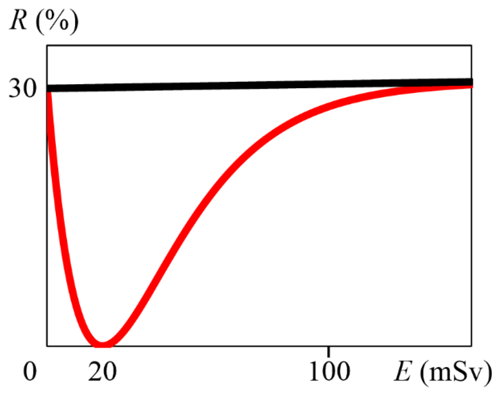
Solving Equation (12) using Grapher 2.5 (Mac OS 10.10.5), we obtained that A is 5.09, so a is 5.09 ×   10 2 . From Equation (7), M is 20 mSv. Therefore, Equation (4) implies Equation (13), which is graphed in Figure 1. From the above, it can be determined that the cumulative radiation dose at which the hormesis effect is maximized is approximately 20 mSv.
R = 30 + 0.005 E 4.15 E e 0.0509 E

2.2. A Sequential General Model Reaction When the Two Rate Constants Are Different

In Section 2.1, we showed that the component Q in Scheme 1 obeys Equation (3). However, it is not common for two reaction rate constants to be the same. Therefore, we considered a general model in which the two reaction constants are different (Scheme 2). Following the well-known differential equations, we obtained Equation (14), where P(0) is the initial component amount of component P, and the rate constants a and b are positive. This equation yields a hunchback graph with one inflection point.
Q E = P 0 a b a e a E e b E
From Equations (2) and (14) and the definition K = kP(0), Equation (15) is obtained:
R = R 0 + ρ E K a b a e a E e b E
As shown in Appendix A, the increase in risk from 0 mSv to N mSv can be ignored. Therefore, Equation (15) may be approximated by Equation (16), similar to that shown in Section 2.1:
R R 0 K a b a e a E e b E
Here, the new function q(E) is defined by Equation (17):
q E : = K a b a e a E e b E
As in Section 2.1, when E is M, the value of q is its maximum, R0. M is solved for as follows:
M = l n b l n a b a    
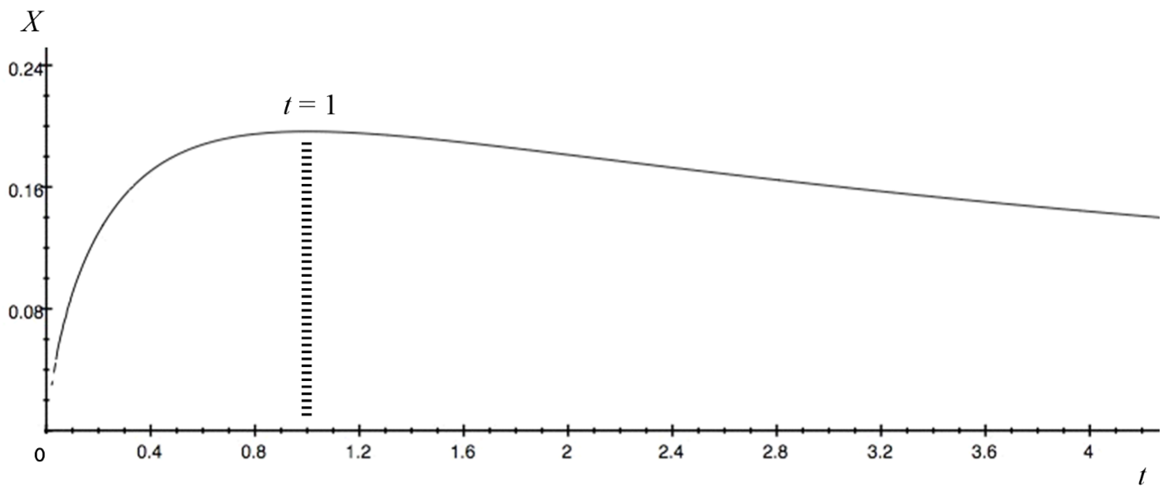
Here, the value obtained by dividing b by a is defined as t (t > 0). The detailed derivation of the following equations is shown in Appendix B.1. As in Section 2.1, we set R0 = 30%, N = 100 mSv, and error = 10% (0 < M < 100). The relational expression between t and X is finally derived. Figure 2 shows Equation (19) plotted using Grapher 2.5:
t t t 1 1 t 1 t B t B t = 0.085 ,           B : = 1 X t 1
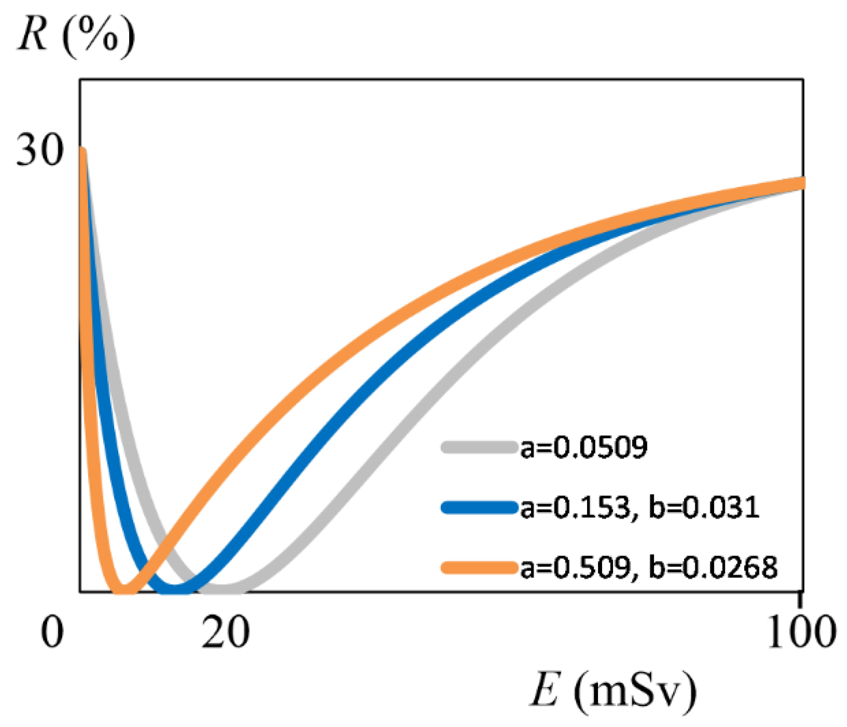
By definition, t represents the relationship between a and b, and X is 1/100 of the dose M at which the hormesis effect is maximized. From the results in Figure 2, we can see that as the relationship between a and b changes, the dose M at which the hormesis effect is maximized changes. What we are most interested in next is how large the dose M can be. From the results in Figure 2, when t is 1, X reaches its maximum of 0.196. Therefore, M is 20 mSv. Although not surprising, this value is the same as the conclusion in Section 2.1. From the graph, in the range where t is greater than 0.947 and less than 1.056, X is 0.196. When t is 0.947, a is 0.0523 and b is 0.0496. When t is 1.056, a is 0.0496 and b is 0.0523. Thus, if the lower-limit value of the risk’s error is fixed, the dose M is maximum in the range where the difference between the formation rate constant a and the decomposition rate constant b of component Q is 5% or less. The greater the difference between a and b, the lower the dose M becomes. For example (see Appendix B.2 for details), when the original a (a = 0.0509) is tripled, b = 0.031 and M = 13 mSv (Figure 3, blue line). Multiplying the original a by 10 yields b = 0.0268, and M becomes 6 mSv (Figure 3, orange line). Therefore, in order to make radiation exposure more advantageous for humans, it is desirable to search for the component Q with almost the same rate constants a and b.

2.3. Changing of Section 2.1’s Error and NOAEL Values

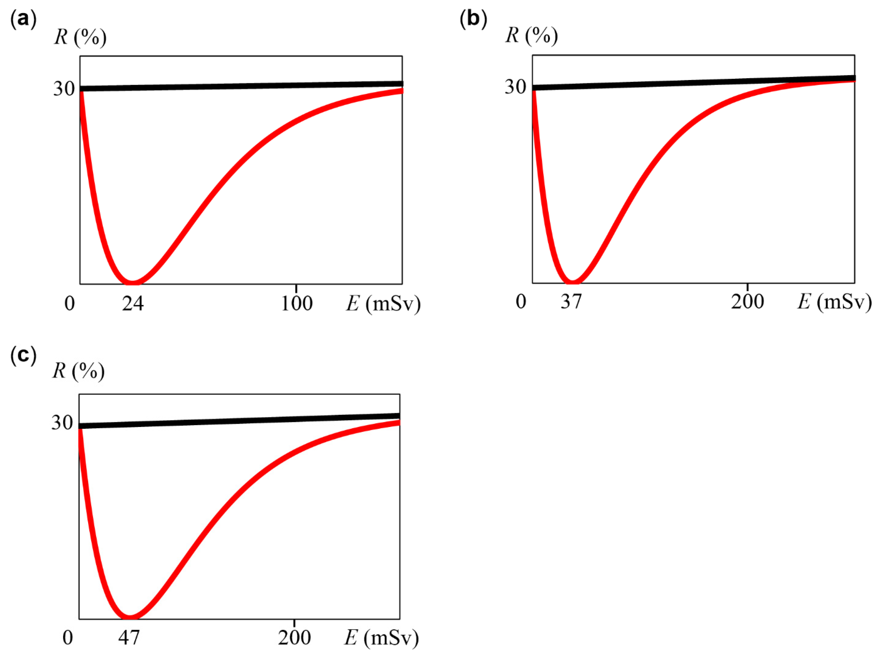
Here, we considered the case where the error value and NOAEL value set in Section 2.1 were changed. First, NOAEL remained at 100 mSv and the error value was changed to 20%. When we allow an error of 20%, 30.5% is multiplied by 0.8 to obtain 24.4% as the risk at 100 mSv. Therefore, we subtracted 24.4% from 30% to obtain 5.6% as q(100). As in Section 2.1, we calculated a using Grapher 2.5, and then a was 0.0409. Thus, Equation (20) was obtained as a function of R. We mathematically obtained that M is 24 mSv using graphical calculation. A graph of Equation (20) is shown in Figure 4a:
R = 30 + 0.005 E 3.34 E e 0.0409 E
Next, when NOAEL was 200 mSv and the error value was 10%, the risk R was obtained. Here, 31% was multiplied by 0.9 to obtain 27.9% as the risk at 200 mSv. Therefore, we obtained 2.1% as q(100). Using Grapher 2.5, a was 0.0267, and Equation (21) and Figure 4b were obtained. Thus, M was 37 mSv. Similarly, when NOAEL was 200 mSv and the error value was 20%, Equation (22) and Figure 4c were obtained, and M was 47 mSv:
R = 30 + 0.005 E 2.19 E e 0.0267 E
R = 30 + 0.005 E 1.71 E e 0.0209 E
Thus, the dose M that maximizes a risk-reducing factor naturally changed when the NOAEL and the error were changed. Although not cumulative doses, other researchers have reported that a best annual effective dose was 60 mSv [81] and that an optimal single absorbed dose was 25 mGy [66]. In the future, it will be necessary to construct a new model that takes the dose rate into account, but if we choose the NOAEL and error appropriately in our kinetic model, the risk-reducing factor that induces hormesis effects in systems used by other researchers may be able to be identified.

2.4. An Example of Applying Our Model to Existing Data

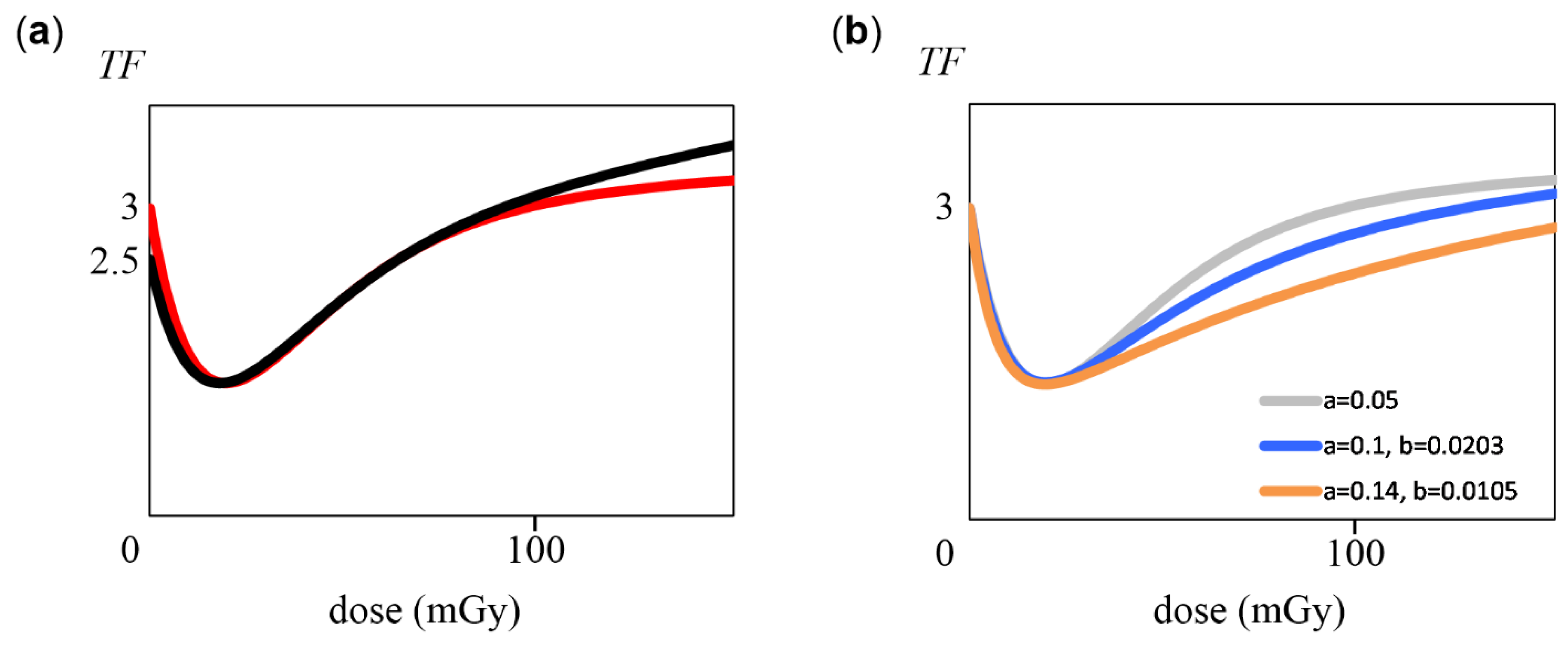
Ref. [34] contains many data points, but basically most of them have large error bars. In our theory, short error bars are acceptable, but data with long error bars are inappropriate. Still, in the Figure 2.8 of Ref. [34] (60 kVp X-rays), we used an experimental result [82] that has short error bars. Assume that we applied the equations obtained in Section 2.1 and Section 2.2 to the data used this time. That is, E is assumed to be an absorbed dose instead of a cumulative effective dose, and R is assumed to be a transformation frequency (TF). If we read from the data that TF is 3 at 0 mGy and 3.7 at 360 mGy, we obtain TF = 3 + 0.00194E, which corresponds to Equation (1). Since M is 20 mGy and TF = 1.3, the following Equation (23) (Figure 5a, red line) is obtained by calculations, as in Section 2.1. According to Equation (23), TF(160) = 3.30, which is within the range of the error bar of the measured value [34,82]. It was also determined that the NOAEL is 96 mGy.
T F = 3 + 0.00194 E 0.236 E e 0.05 E
On the other hand, a different line can be obtained from TF(0) = 2.5 and TF(160) = 3.7. Using the value 1.3 when M = 20 mGy, Equation (24) was obtained. TF(360) = 5.2 obtained from this equation is appropriate because it is within the error bar range of the experimental value. The graph is shown in Figure 5a (black line). NOAEL was 64 mGy.
T F = 2.5 + 0.0075 E 0.183 E e 0.05 E
Next, based on Equation (15), we considered two different rate constants, as in Scheme 2. At this time, we considered how far the two rate constants can be changed within the range of the error bar. For example, when a is set to 0.1, two-fold of the original 0.05, b = 0.0203 was obtained by graphical calculation in order to keep M at 20 mGy. Equation (25) was obtained from TF(20) = 1.3. TF(160) = 3.18 and TF(360) = 3.69 are values within the range of the error bar, and then Equation (25) (Figure 5b, blue line) is appropriate. NOAEL was 127 mGy.
T F = 3 + 0.00194 E 3.27 e 0.0203 E e 0.1 E
When the lower limit of the error bar for the experimental value of 360 mGy was 3.65, a = 0.14 and b = 0.0105 were found (details are shown in Appendix C). Equation (26) was thus obtained, and the NOAEL was 180 mGy. TF(160) = 2.88 was obtained, which is within the error bar of the experimental value.
T F = 3 + 0.00194 E 2.32 e 0.0105 E e 0.14 E
Thus, even in cases where the error bars are short, this variety of formulas can be used. The theory proposed in this paper can only explain existing experiments with extremely short error bar lengths. Our theory rather provides a policy to find unknown risk-reducing factors in terms of kinetics.

3. Conclusions, Problems, and Implications

We had previously reported a model that suppresses radiation-specific cancer development [69,70,71]. In this paper, we considered reaction kinetic models that suppress radiation-nonspecific cancer. With the special reaction kinetic model (Section 2.1), we considered the case in which the rate constant for the formation of the risk suppressor is the same as the rate constant for its degradation. As a result, the calculations led to a maximum effect of radiation hormesis at 20 mSv.
With the general model (Section 2.2), we considered the case where the rate constants for production and decomposition were different. As a result, it was theoretically determined that the dose M at which the effect of radiation hormesis is maximized depends on the relationship between the rate constant for production and the rate constant for decomposition, and that the dose M increased as the values of the two rate constants approached each other. In this case, the dose M reached a maximum of about 20 mSv when the relationship was near identical.
In Section 2.3, when the error value and NOAEL value set in Section 2.1 were changed, the dose M that maximizes a risk-reducing factor changed. In Section 2.4, when an experimental result with short error bars was used, it was assumed that we applied the equations obtained in Section 2.1 and Section 2.2. Even in cases where the error bars are short, several equations can be obtained. Thus, the theory proposed in this paper can only explain existing experiments with extremely short error bar lengths and provides a policy to find unknown risk-reducing factors in terms of kinetics.
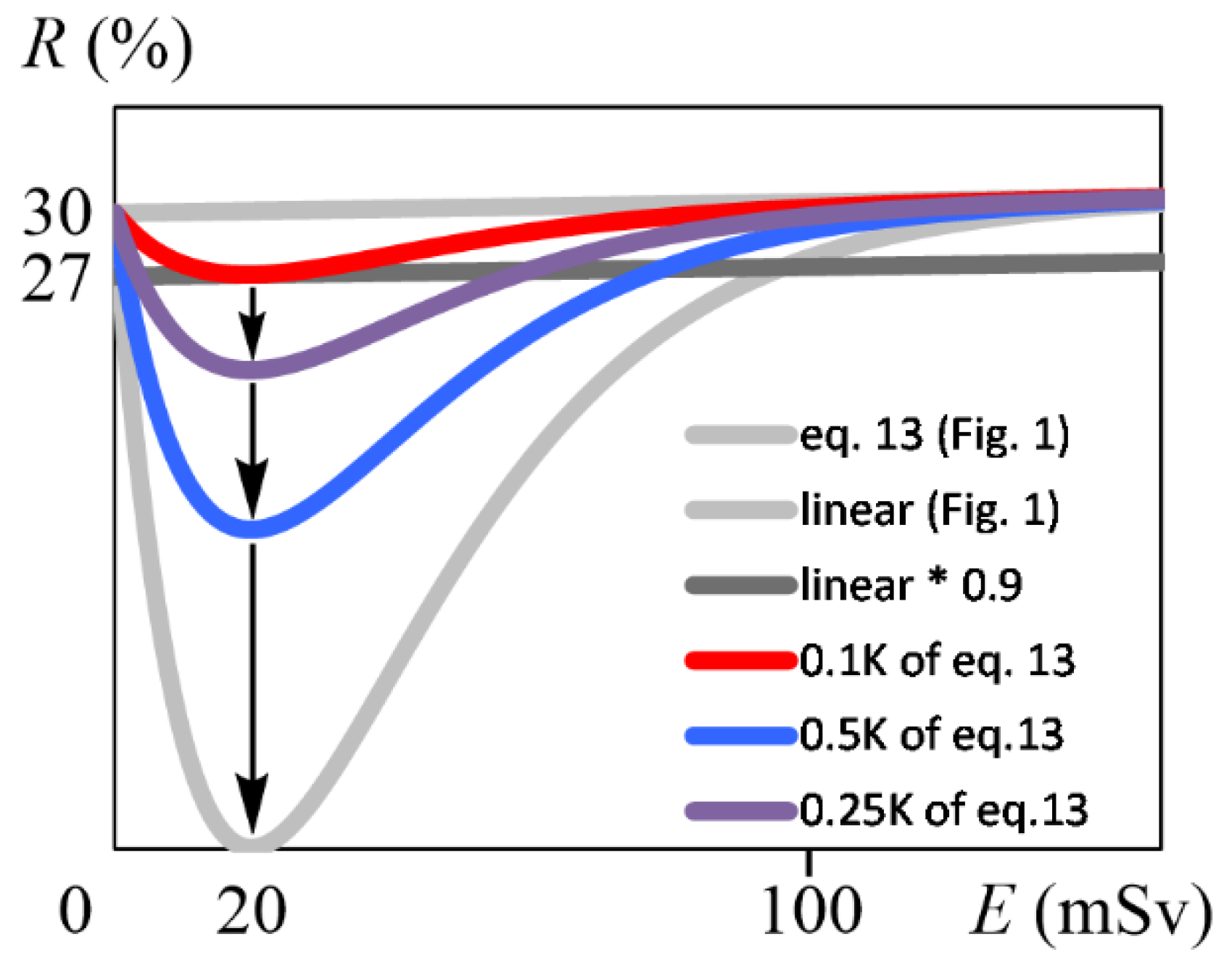
The weakness of the above conclusion Is, of course, that this article is only hypothetical. Equation (13) has the largest hormesis effect as a result of adjusting for k, which links the risk to the risk-reducing factor in Equation (2), and the initial raw material amount P(0). For the hormesis effect to be buried in a linear increase, we must first allow a 10% error in Equation (1) at 20 mSv and the risk must be at least 27.1%. Applying a = 0.0509 and R = 27.1% to Equation (4), Equation (27) (Figure 6, red line) was obtained. From Figure 6, Equation (27) shows that the risk increased linearly with the dose when a 10% error was allowed in R:
R = 30 + 0.005 E 0.417 E e 0.0509 E
Equation (27) is the case where k and P(0) in Equation (13) were very small. In the future, if k or P(0) can be increased, a hormesis effect will appear at low doses. For example, if an unknown factor is found that is maximal at 20 mSv, such a factor may be a risk-reducing factor, and its overexpression in vivo would reduce risk; then, the model proposed in this paper is justified. Of course, it is not realistic to maximize the risk-reducing factor (Figure 6, gray curved line), and it would be possible to partially observe hormesis effects by increasing K, as seen in the purple and blue lines in Figure 6. Thus, the exploration and overexpression of such risk-reducing factors obeying the kinetic model of this paper may lead to the development of cancer-reducing therapeutic modalities. If cancer suppression by such factors is achieved, it is expected that the perspective on low doses will change. These factors may be found by exploring unknown substances present in radioresistant bacterium [83], radio-tolerant hyper-thermophilic archaea [84], and radio-tolerant tardigrades [85]. In addition to proteins, risk-reducing factors may include some DNA damage [1,2] causing mutations [86] that are less likely to lead to cancer. For example, 2,5-diamino-4H-imidazol-4-one (Iz) and 2,2,4-triamino-5(2H)-oxazolone (Oz) can be produced by γ radiation or other oxidations [87], and the biological implications of these damages have been analyzed in vitro [86,88,89,90,91,92,93]. Such DNA damages may be relatively safe for living organisms.

Funding

The idea described in this manuscript was obtained on the basis of my other studies supported by research grants from the Radiation Effects Association, from the Nakatomi Foundation, from KAKENHI (23510069, 17K00558 and 23K11427), and from the Japan Prize Foundation. I am grateful to these foundations.

Institutional Review Board Statement

Not applicable.

Informed Consent Statement

Not applicable.

Data Availability Statement

The author confirms that the data supporting the findings of this study are available within the article.

Acknowledgments

Thank you to the reviewers for their valuable comments.

Conflicts of Interest

The author declares no conflicts of interest.

Abbreviations

NOAELNo Observed Adverse Effect Level
LNTLinear non-threshold
EPAEnvironmental Protection Agency
PROFACProtection Factor
TFTransformation frequency
Iz2,5-diamino-4H-imidazol-4-one
Oz2,2,4-triamino-5(2H)-oxazolone

Appendix A. Not ignoring the 0.5% increase from 0 mSv to 100 mSv
In the approximation in Section 2.1 using Equation (6), the increment of 0.5 for 0 mSv to 100 mSv was ignored. In the current section, Equation (4) is used without neglecting this increment. We allow an error of 0.1, so 30.5% is multiplied by 0.9 to obtain 27.45% at 100 mSv. Substituting this value into Equation (4) yields Equation (A1), which when reorganized becomes Equation (A2):
27.45 = 30 + 0.5 100 K a e 100 a
K a = 0.0305 e 100 a
Substituting Equation (A2) into Equation (4) yields Equation (A3):
R = 30 + 0.005 E 0.0305 E e a 100 E
As the definition of M, when E is M, the risk is its minimum, 0 (Equation A4). Differentiating Equation (A3) yields Equation (A5). Since Equations (A4) and (A6) both hold, Equations (A7) and (A8) follow:
R M = 0
d R d E = 0.005 0.0305 1 a E e a 100 E
d R d E M = 0
30 + 0.005 M 0.0305 M e a 100 M = 0
0.005 0.0305 1 a M e a 100 M = 0
From Equations (A7) and (A8), eliminating the exponential term yields Equation (A9). (Note: This M is different from the M in Section 2.1, so 1 − aM is not zero.)
30 + 0.005 M = 0.005 M 1 a M
This equation can be rearranged into Equation (A10), which is quadratic in M. Furthermore, solving Equation (A10) yields Equation (A11):
a M 2 + 6000 a M 6000 = 0
M = 3000 1 + 1 1500 a 0.5 3000
Substituting Equation (A11) into Equation (A8) establishes Equation (A12), using the new definition provided in Equation (A13) and recalling that 100a = A (A > 1):
e A 30 A β = 0.164 1 1 30 A β
β : = 1 + 1 15 A 0.5 1
Using Equations (A12) and (A13), we can find A using Grapher 2.5. Note that since M is greater than 0 and less than 100, beta is less than 1/30, and from Equation (A13), A is greater than 0.984.
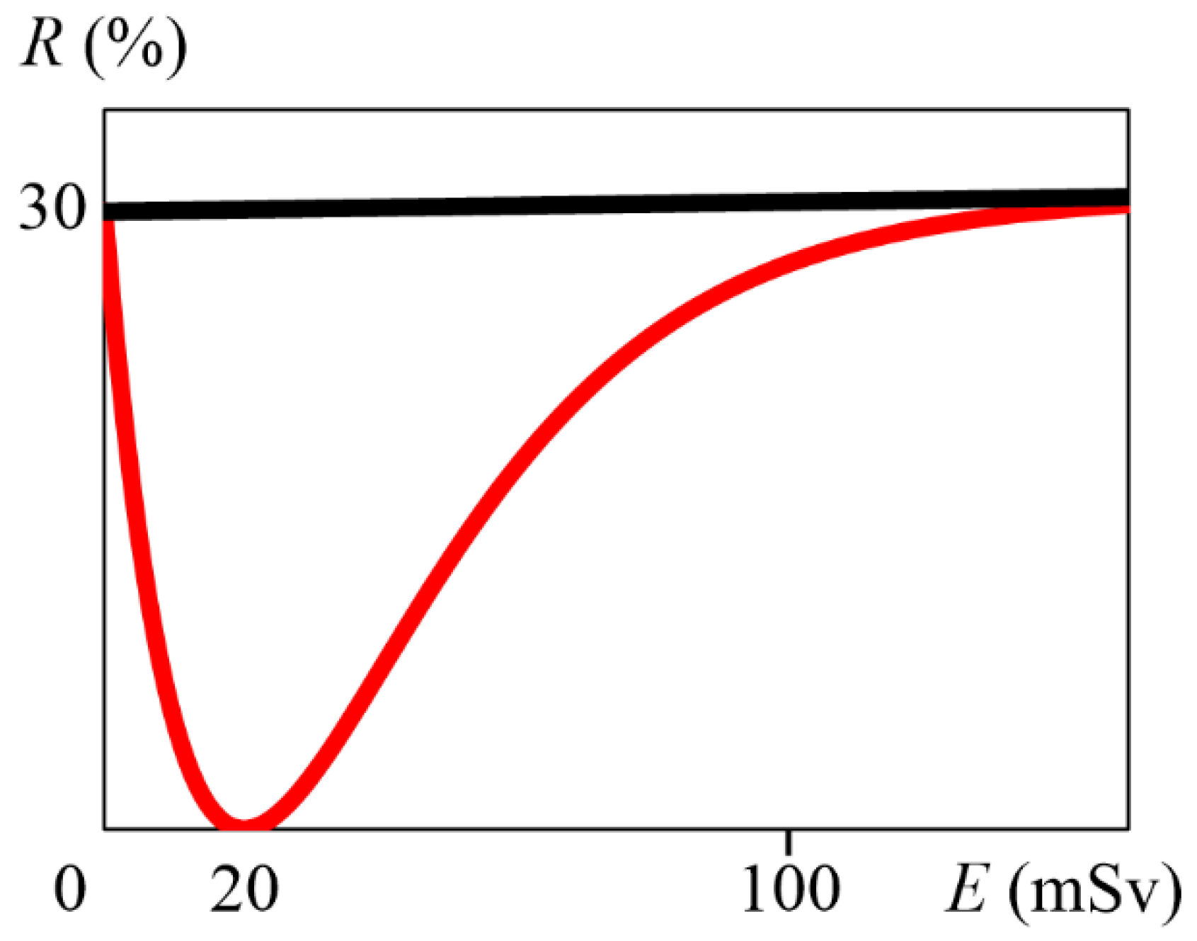
The result shows that A is 4.87, implying that a is 0.0487. Using Equation (A11), we obtain that M is 20 mSv. Equation (A3) can thus be expressed as Equation (A14), which was graphed using Grapher 2.5 to obtain the risk at 20 mSv, which is almost zero (Figure A1):
R = 30 + 0.005 E 3.99 E e 0.0487 E
The dose at which the hormesis effect is maximized is approximately 20 mSv, which is the same dose as in Section 2.1 when considering two significant digits. This indicates that the increase from 0 mSv to 100 mSv can be disregarded.
Figure A1. Graph of Equation (A14), with E (mSv) on the horizontal axis and R (%) on the vertical axis. The red line indicates Equation (A14), and the black line indicates R = 30 + 0.005E.
Radiation 04 00006 g0a1

Appendix B

Appendix B.1. Derivation of Equation (19)

By the definition of t, Equation (18) (Section 2.2) can be rewritten as Equation (A15), and the value of q when E is M can be found, as shown by the sequence of steps in Equation (A16):
M = l n t a t 1
q M = K 1 t 1 e a M e a t M = K 1 t 1 e l n t t 1 e t l n t t 1 = K 1 t 1 t 1 t 1 t t t 1 = K 1 t 1 t 1 t 1 1 t 1 = K t t t 1
When E is M, the value of q is R0, and the following equation is obtained:
K t t t 1 = R 0
Here, we perform specific numerical calculations for the case of Ref. [74]. We set NOAEL to 100 mSv. As in Section 2.1, q(100) is 2.55, so Equation (A18) can be derived as shown from Equation (17) and the definition of t:
q 100 = K 1 t 1 e 100 a e 100 a t = 2.55
By eliminating K using Equation (A17) and R0 = 30, Equation (A19) can be derived:
t t t 1 1 t 1 e 100 a e 100 a t = 0.085
Recalling that 100a = A (A > 0), Equation (A19) becomes Equation (A20):
t t t 1 1 t 1 e A e A t = 0.085
To make it easier to interpret the graph (Figure 2), we newly define X as the value obtained by dividing M by 100 (0 < X < 1). From Equation (A15) and the definition of A, X becomes that shown in Equation (A21). From Equation (A21), A is expressed in terms of X and t, as shown in Equation (A22). From Equations (A20) and (A22), B is newly defined, and Equation (19) is derived (in Section 2.2):
X = l n t 100 a t 1 = l n t A t 1
A = l n t X t 1

Appendix B.2. Details of Figure 3

Also see Section 2.2. When a = 0.153, t = 0.203 is found by graphical calculation from Equation (A19). Thus, b = 0.0310 is obtained. Additionally, according to Equation (A17), K is 45.0. Thus, Equation (A23) is obtained, and M is 13 mSv:
R = 30 + 0.005 E 56.5 e 0.031 E e 0.153 E
Similarly, when a = 0.509, we obtain, in order, t = 0.0527, b = 0.0268, and K = 35.3. The equation for R in this case is as follows, and M is 6 mSv:
R = 30 + 0.005 E 37.3 e 0.0268 E e 0.509 E

Appendix C. Derivation of Equation (26)

Also see Section 2.4. If a > b, then exp(−aE) << exp(−bE). Equation (15) is approximated, as shown in Equation (A25) below:
T F = 3 + 0.00194 E K a b a e a E e b E 3 + 0.00194 E K e b E
From TF(20) = 1.3 and TF(360) = 3.65, Equations (A26) and (A27) are obtained:
1.3 = 3 + 0.00194 × 20 K e 20 b
3.65 = 3 + 0.00194 × 360 K e 360 b
From Equations (A26) and (A27), if K is eliminated, we obtain b = 0.0105. Substituting the value of b and M = 20 mGy into Equation (18) yields a = 0.140. From TF(20) = 1.3, Ka/(ba) = −2.32 is obtained. Therefore, Equation (26) is obtained.

Appendix D. Equations of Figure 6

Also see Section 3. Equation (A28) is the function of the purple curved line in Figure 6:
R = 30 + 0.005 E 1.04 E e 0.0509 E
Equation (A29) is that of the blue curved line in Figure 6:
R = 30 + 0.005 E 2.08 E e 0.0509 E

References

  1. Friedberg, E.C.; Walker, G.C.; Siede, W.; Wood, R.D.; Schultz, R.A.; Ellenberger, T. DNA Repair and Mutagenesis, 2nd ed.; ASM Press: Washington, DC, USA, 2006. [Google Scholar]
  2. Greenberg, M.M. Radical and Radical Ion Reactivity in Nucleic Acid Chemistry; John Wiley & Sons, Inc.: Hoboken, NJ, USA, 2009. [Google Scholar]
  3. Rhim, J.S.; Thraves, P.; Dritschilo, A.; Kuettel, M.R.; Lee, M.S. Radiation-induced neoplastic transformation of human cells. Scanning Microsc. 1993, 7, 209–215; discussion 215–216. [Google Scholar]
  4. Elmore, E.; Lao, X.Y.; Kapadia, R.; Redpath, J.L. The effect of dose rate on radiation-induced neoplastic transformation in vitro by low doses of low-LET radiation. Radiat. Res. 2006, 166, 832–838. [Google Scholar] [CrossRef]
  5. Raabe, O.R. Concerning radiation carcinogenesis. Health Phys. 2014, 107, 571. [Google Scholar] [CrossRef]
  6. Tubiana, M. Can we reduce the incidence of second primary malignancies occurring after radiotherapy? A critical review. Radiother. Oncol. 2009, 91, 4–15; discussion 1–3. [Google Scholar] [CrossRef]
  7. Preston, D.L.; Ron, E.; Tokuoka, S.; Funamoto, S.; Nishi, N.; Soda, M.; Mabuchi, K.; Kodama, K. Solid cancer incidence in atomic bomb survivors: 1958–1998. Radiat. Res. 2007, 168, 1–64. [Google Scholar] [CrossRef]
  8. ICRP. Low-Dose Extrapolation of Radiation-Related Cancer Risk. ICRP Publication 99. International Commission on Radiological Protection; Elsevier Oxford: Amsterdam, The Netherlands, 2006. [Google Scholar]
  9. UNSCEAR. Summary of Low-Dose Radiation Effects on Health; UNSCEAR 2010 Report; United Nations Publications: New York, NY, USA, 2010. [Google Scholar]
  10. Tubiana, M.; Arengo, A.; Averbeck, D.; Masse, R. Low-dose risk assessment. Radiat. Res. 2007, 167, 742–744. [Google Scholar] [CrossRef]
  11. Mossman, K.L. Economic and policy considerations drive the LNT debate. Radiat. Res. 2008, 169, 245. [Google Scholar] [CrossRef]
  12. Leonard, B.E. Common sense about the linear no-threshold controversy-give the general public a break. Radiat. Res. 2008, 169, 245–246, Erratum in Radiat. Res. 2008, 169, 606. [Google Scholar] [CrossRef] [PubMed]
  13. Tubiana, M.; Aurengo, A.; Averbeck, D.; Masse, R. Low-dose risk assessment: The debate continues. Radiat. Res. 2008, 169, 246–247. [Google Scholar] [CrossRef]
  14. Feinendegen, L.E.; Paretzke, H.; Neumann, R.D. Two principal considerations are needed after low doses of ionizing radiation. Radiat. Res. 2008, 169, 247–248. [Google Scholar] [CrossRef] [PubMed]
  15. Mothersill, C.; Seymour, C. Low dose radiation mechanisms: The certainty of uncertainty. Mutat. Res. Genet. Toxicol. Environ. Mutagen. 2022, 876, 503451. [Google Scholar] [CrossRef]
  16. Boice, J.D.J. The linear nonthreshold (LNT) model as used in radiation protection: An NCRP update. Int. J. Radiat. Biol. 2017, 93, 1079–1092. [Google Scholar] [CrossRef]
  17. Environmental Protection Agency (EPA). Proposed rule. Strengthening transparency in regulatory science. Fed. Reg. 2018, 83, 18768–18774. [Google Scholar]
  18. Calabrese, E.J.; Hanekamp, J.C.; Shamoun, D.Y. The EPA cancer risk assessment default model proposal: Moving away from the LNT. Dose Response 2018, 16, 1559325818789840. [Google Scholar] [CrossRef]
  19. Olivieri, G.; Bodycote, J.; Wolff, S. Adaptive response of human lymphocytes to low concentrations of radioactive thymidine. Science 1984, 223, 594–597. [Google Scholar] [CrossRef]
  20. Wolff, S. The adaptive response in radiobiology: Evolving insights and implications. Environ. Health Perspect. 1998, 106 (Suppl. S1), 277–283. [Google Scholar] [PubMed]
  21. Azzam, E.I.; Raaphorst, G.P.; Mitchel, R.E. Radiation-induced adaptive response for protection against micronucleus formation and neoplastic transformation in C3H 10T1/2 mouse embryo cells. Radiat. Res. 1994, 138, S28–S31. [Google Scholar] [CrossRef] [PubMed]
  22. Shadley, J.D. Chromosomal adaptive response in human lymphocytes. Radiat. Res. 1994, 138, S9–S12. [Google Scholar] [CrossRef] [PubMed]
  23. Thierens, H.; Vral, A.; Barbé, M.; Meijlaers, M.; Baeyens, A.; Ridder, L.D. Chromosomal radiosensitivity study of temporary nuclear workers and the support of the adaptive response induced by occupational exposure. Int. J. Radiat. Biol. 2002, 78, 1117–1126. [Google Scholar] [CrossRef] [PubMed]
  24. Tapio, S.; Jacob, V. Radioadaptive response revisited. Radiat. Environ. Biophys. 2007, 46, 1–12. [Google Scholar] [CrossRef]
  25. Guéguen, Y.; Bontemps, A.; Ebrahimian, T.G. Adaptive responses to low doses of radiation or chemicals: Their cellular and molecular mechanisms. Cell. Mol. Life Sci. 2019, 76, 1255–1273. [Google Scholar] [CrossRef]
  26. Devic, C.; Ferlazzo, M.L.; Foray, N. Influence of individual radiosensitivity on the adaptive response phenomenon: Toward a mechanistic explanation based on the nucleo-shuttling of atm protein. Dose Response 2018, 16, 1559325818789836. [Google Scholar] [CrossRef]
  27. Agathokleous, E.; Calabrese, E.J.; Barcelo, D. Environmental hormesis: New developments. Sci. Total Environ. 2024, 906, 167450. [Google Scholar] [CrossRef]
  28. Joiner, M.C.; Lambin, P.; Malaise, E.P.; Robson, T.; Arrand, J.E.; Skov, K.A.; Marples, B. Hypersensitivity to very-low single radiation doses: Its relationship to the adaptive response and induced radioresistance. Mutat. Res. 1996, 358, 171–183. [Google Scholar] [CrossRef] [PubMed]
  29. Dimova, E.G.; Bryant, P.E.; Chankova, S.G. “Adaptive response”—Some underlying mechanisms and open questions. Genet. Mol. Biol. 2008, 31, 396–408. [Google Scholar] [CrossRef]
  30. UNSCEAR. Sources and Effects of Ionizing Radiation. Annex B: Adaptive Responses to Radiation in Cells and Organisms; UNSCEAR 1994 Report; United Nations Publications: New York, NY, USA, 1994. [Google Scholar]
  31. UNSCEAR. Sources, Effects and Risks of Ionizing Radiation. Annex C: Biological Mechanisms Relevant for the Inference of Cancer Risks from Low-Dose and Low-Dose-Rate Radiation. Section III.F.4 Adaptive Response; UNSCEAR 2020/2021 Report Volume III; United Nations Publications: New York, NY, USA, 2022. [Google Scholar]
  32. Socol, Y.; Dobrzynski, L.; Doss, M.; Feinendegen, L.E.; Janiak, M.K.; Miller, M.L.; Sanders, C.L.; Scott, B.R.; Ulsh, B.; Vaiserman, A. Commentary: Ethical issues of current health-protection policies on low-dose ionizing radiation. Dose Response 2014, 12, 342–348. [Google Scholar] [CrossRef] [PubMed]
  33. Luckey, T.D. Radiation Hormesis; CRC Press: Boca Raton, FL, USA, 1991. [Google Scholar]
  34. Sanders, C.L. Radiation Hormesis and the Linear-No-Threshold Assumption; Springer: Berlin, Germany, 2010. [Google Scholar]
  35. Feinendegen, L.E.; Bond, V.P.; Sondhaus, C.A. The dual response to low-dose irradiation: Induction vs. prevention of DNA damage. In Biological Effects of Low Dose Radiation. Excerpta Medica. International Congress Series 1211; Yamada, T., Mothersill, C., Michael, B.D., Potten, C.S., Eds.; Elsevier: Amsterdam, The Netherlands, 2000; pp. 3–17. [Google Scholar]
  36. Sutou, S. A message to Fukushima: Nothing to fear but fear itself. Genes Environ. 2016, 38, 12. [Google Scholar] [CrossRef]
  37. Sutou, S. The 10th anniversary of the publication of genes and environment: Memoir of establishing the Japanese environmental mutagen society and a proposal for a new collaborative study on mutagenic hormesis. Genes Environ. 2017, 39, 9. [Google Scholar] [CrossRef]
  38. Sutou, S. Low-dose radiation from A-bombs elongated lifespan and reduced cancer mortality relative to un-irradiated individuals. Genes Environ. 2018, 40, 26. [Google Scholar] [CrossRef]
  39. Sutou, S.; Koeda, A.; Komatsu, K.; Shiragiku, T.; Seki, H.; Yamakage, K.; Niitsuma, T.; Kudo, T.; Wakata, A. Collaborative study of thresholds for mutagens: Proposal of a typical protocol for detection of hormetic responses in cytotoxicity tests. Genes Environ. 2018, 40, 20. [Google Scholar] [CrossRef]
  40. Rattan, S.I.S.; Bourg, E.L. Hormesis in Health and Disease; CRC Press, Inc.: Boca Raton, FL, USA, 2014. [Google Scholar]
  41. Lampe, N.; Breton, V.; Sarramia, D.; Sime-Ngando, T.; Biron, D.G. Understanding low radiation background biology through controlled evolution experiments. Evol. Appl. 2017, 10, 658–666. [Google Scholar] [CrossRef]
  42. Feinendegen, L.E. Evidence for beneficial low level radiation effects and radiation hormesis. Br. J. Radiol. 2005, 78, 3–7. [Google Scholar] [CrossRef]
  43. Scott, B.R. Stochastic thresholds: A novel explanation of nonlinear dose-response relationships for stochastic radiobiological effects. Dose Response 2006, 3, 547–567. [Google Scholar] [CrossRef]
  44. Scott, B.R. Modeling DNA double-strand break repair kinetics as an epiregulated cell-community-wide (epicellcom) response to radiation stress. Dose Response 2011, 9, 579–601. [Google Scholar] [CrossRef]
  45. Scott, B.R.; Belinsky, S.A.; Leng, S.; Lin, Y.; Wilder, J.A.; Damiani, L.A. Radiation-stimulated epigenetic reprogramming of adaptive-response genes in the lung: An evolutionary gift for mounting adaptive protection against lung cancer. Dose Response 2009, 7, 104–131. [Google Scholar] [CrossRef]
  46. Leonard, B.E.; Thompson, R.E.; Beecher, G.C. Human lung cancer risks from radon—Part II—Influence from combined adaptive response and bystander effects—A microdose analysis. Dose Response 2011, 9, 502–553. [Google Scholar] [CrossRef]
  47. Schöllnberger, H.; Stewart, R.D.; Mitchel, R.E.; Hofmann, W. An examination of radiation hormesis mechanisms using a multistage carcinogenesis model. Nonlinearity Biol. Toxicol. Med. 2004, 2, 317–352. [Google Scholar] [CrossRef]
  48. Zhao, Y.; Ricci, P.F. Modeling dose-response at low dose: A systems biology approach for ionization radiation. Dose Response 2010, 8, 456–477. [Google Scholar] [CrossRef]
  49. Feinendegen, L.E.; Paretzke, H.G.; Neumann, R.D. Damage propagation in complex biological systems following exposure to low doses of ionising radiation. At. Peace Int. J. 2007, 1, 336–354. [Google Scholar] [CrossRef]
  50. Feinendegen, L.E.; Pollycove, M.; Neumann, R.D. Low-dose cancer risk modeling must recognize up-regulation of pro-tection. Dose Response 2009, 8, 227–252. [Google Scholar] [PubMed]
  51. Dobrzyński, L.; Fornalski, K.W.; Socol, Y.; Reszczyńska, J.M. Modeling of irradiated cell transformation: Dose- and time-dependent effects. Radiat. Res. 2016, 186, 396–406. [Google Scholar] [CrossRef] [PubMed]
  52. Leblanc, J.E.; Burtt, J.J. Radiation biology and its role in the Canadian radiation protection framework. Health Phys. 2019, 117, 319–329. [Google Scholar] [CrossRef]
  53. UNSCEAR. Sources and Effects of Ionizing Radiation. United Nations Scientific Committee on the Effects of Atomic Radiation; UNSCEAR 2000 Report; United Nations Publications: New York, NY, USA, 2000. [Google Scholar]
  54. NCRP. Evaluation of the Linear-Nonthreshold Dose-Response Model for Ionizing Radiation; NCRP Report No. 136; National Council on Radiation Protection and Measurements: Bethesda, MD, USA, 2001. [Google Scholar]
  55. Scott, B.R.; Haque, M.; Palma, J.D. Biological basis for radiation hormesis in mammalian cellular communities. Int. J. Low Radiat. 2007, 4, 1–20. [Google Scholar] [CrossRef]
  56. Fornalski, K.W. Radiation adaptive response and cancer: From the statistical physics point of view. Phys. Rev. E. 2019, 99, 022139. [Google Scholar] [CrossRef]
  57. Uchinomiya, K.; Yoshida, K.; Kondo, M.; Tomita, M.; Iwasaki, T. A mathematical model for stem cell competition to maintain a cell pool injured by radiation. Radiat. Res. 2020, 194, 379–389. [Google Scholar] [CrossRef]
  58. Kim, S.B.; Sanders, N. Model averaging with AIC weights for hypothesis testing of hormesis at low doses. Dose Response 2017, 15, 1559325817715314. [Google Scholar] [CrossRef]
  59. Kim, S.B.; Bartell, S.M.; Gillen, D.L. Inference for the existence of hormetic dose-response relationships in toxicology studies. Biostatistics 2016, 17, 523–536. [Google Scholar] [CrossRef]
  60. Esposito, G.; Campa, A.; Pinto, M.; Simone, G.; Tabocchini, M.A.; Belli, M. Adaptive response: Modelling and experimental studies. Radiat. Prot. Dosim. 2011, 143, 320–324. [Google Scholar] [CrossRef] [PubMed]
  61. Wodarz, D.; Sorace, R.; Komarova, N.L. Dynamics of cellular responses to radiation. PLoS Comput. Biol. 2014, 10, e1003513. [Google Scholar] [CrossRef]
  62. Socol, Y.; Shaki, Y.Y.; Dobrzyński, L. Damped-oscillator model of adaptive response and its consequences. Int. J. Low Rad. 2020, 11, 186–206. [Google Scholar] [CrossRef]
  63. Smirnova, O.A.; Yonezawa, M. Radioprotection effect of low level preirradiation on mammals: Modeling and experimental investigations. Health Phys. 2003, 85, 150–158. [Google Scholar] [CrossRef]
  64. Scott, B.R. First generation stochastic gene episilencing (step1) model and applications to in vitro carcinogen exposure. Dose Response 2013, 11, 9–28. [Google Scholar] [CrossRef]
  65. Leonard, B.E. A review: Development of a microdose model for analysis of adaptive response and bystander dose response behavior. Dose Response 2008, 6, 113–183. [Google Scholar] [CrossRef]
  66. Fornalski, K.W.; Adamowski, Ł.; Dobrzyński, L.; Jarmakiewicz, R.; Powojska, A.; Reszczyńska, J. The radiation adaptive response and priming dose influence: The quantification of the Raper-Yonezawa effect and its three-parameter model for postradiation DNA lesions and mutations. Radiat. Environ. Biophys. 2022, 61, 221–239. [Google Scholar] [CrossRef]
  67. Fornalski, K.W. Radioadaptation and radioresistance during deep space travels. J. Space Saf. Eng. 2022, 9, 385–389. [Google Scholar] [CrossRef]
  68. Schöllnberger, H.; Ménache, M.G.; Hanson, T.E. A biomathematical modeling approach to explain the phenomenon of radiation hormesis. Hum. Ecol. Risk Assess. Int. J. 2001, 7, 867–890. [Google Scholar] [CrossRef]
  69. Kino, K. The prospective mathematical idea satisfying both radiation hormesis under low radiation doses and linear non-threshold theory under high radiation doses. Gene Environ. 2020, 42, 4. [Google Scholar] [CrossRef]
  70. Kino, K.; Ohshima, T.; Takeuchi, H.; Kobayashi, T.; Kawada, T.; Morikawa, M.; Miyazawa, H. Considering existing factors that may cause radiation hormesis at <100 mSv and obey the linear no-threshold theory at ≥100 mSv. Challenges 2021, 12, 33. [Google Scholar]
  71. Kino, K. The radiation-specific components generated in the second step of sequential reactions have a mountain-shaped function. Toxics 2023, 11, 301. [Google Scholar] [CrossRef]
  72. Calabrese, E.J.; Shamoun, D.Y.; Hanekamp, J.C. Cancer risk assessment: Optimizing human health through linear dose-response models. Food Chem. Toxicol. 2015, 81, 137–140. [Google Scholar] [CrossRef]
  73. Scott, B.R. Residential radon appears to prevent lung cancer. Dose Response 2011, 9, 444–464. [Google Scholar] [CrossRef] [PubMed]
  74. Ministry of the Environment, Japan. Uniform Basic Information on Health Effects of Radiation, Etc. 2016 Edition Ver.2017001. Available online: https://www.env.go.jp/chemi/rhm/h28kisoshiryo/h28kiso-03-07-03.html (accessed on 13 December 2023).
  75. ICRP. The 2007 Recommendations of the International Commission on Radiological Protection; ICRP Publication 103; Elsevier Oxford: Amsterdam, The Netherlands, 2007. [Google Scholar]
  76. Raper, J.R. Effects of total surface beta irradiation. Radiology 1947, 49, 314–324. [Google Scholar] [CrossRef] [PubMed]
  77. Feinendegen, L.E. Low doses of ionizing radiation: Relationship between biological benefit and damage induction. A synopsis. World J. Nucl. Med. 2005, 4, 21–34. [Google Scholar]
  78. Agathokleous, E.; Kitao, M.; Calabrese, E.J. Environmental hormesis and its fundamental biological basis: Rewriting the history of toxicology. Environ. Res. 2018, 165, 274–278. [Google Scholar] [CrossRef] [PubMed]
  79. Agathokleous, E.; Saitanis, C.; Markouizou, A. Hormesis shifts the No-Observed-Adverse-Effect Level (NOAEL). Dose Response 2021, 19, 15593258211001667. [Google Scholar] [CrossRef] [PubMed]
  80. Sanders, C.L.; Scott, B.R. Smoking and hormesis as confounding factors in radiation pulmonary carcinogenesis. Dose Response 2008, 6, 53–79. [Google Scholar] [CrossRef]
  81. Luckey, T.D. Documented optimum and threshold for ionising radiation. Int. J. Nucl. Law 2007, 1, 378–409. [Google Scholar] [CrossRef]
  82. Redpath, J. Radiation-induced neoplastic transformation in vitro: Evidence for a protective effect at low doses of low LET radiation. Cancer Metastasis Rev. 2004, 23, 333–339. [Google Scholar] [CrossRef]
  83. Sadowska-Bartosz, I.; Bartosz, G. Antioxidant defense of Deinococcus radiodurans: How does it contribute to extreme radiation resistance? Int. J. Radiat. Biol. 2023, 99, 1803–1829. [Google Scholar] [CrossRef]
  84. Ranawat, P.; Rawat, S. Radiation resistance in thermophiles: Mechanisms and applications. World J. Microbiol. Biotechnol. 2017, 33, 112. [Google Scholar] [CrossRef] [PubMed]
  85. Kasianchuk, N.; Rzymski, P.; Kaczmarek, Ł. The biomedical potential of tardigrade proteins: A review. Biomed. Pharmacother. 2023, 158, 114063. [Google Scholar] [CrossRef]
  86. Kino, K.; Kawada, T.; Hirao-Suzuki, M.; Morikawa, M.; Miyazawa, H. Products of oxidative guanine damage form base pairs with guanine. Int. J. Mol. Sci. 2020, 21, 7645. [Google Scholar] [CrossRef]
  87. Cadet, J.; Berger, M.; Buchko, G.W.; Joshi, P.C.; Raoul, S.; Ravanat, J.-L. 2,2-Diamino-4-[(3,5-di-O-acetyl-2-deoxy-β-D-erythro-pentofuranosyl)amino]-5-(2H)-oxazolone: A novel and predominant radical oxidation product of 3′,5′-di-O-acetyl-2′-deoxyguanosine. J. Am. Chem. Soc. 1994, 116, 7403–7404. [Google Scholar] [CrossRef]
  88. Neeley, W.L.; Delaney, J.C.; Henderson, P.T.; Essigmann, J.M. In vivo bypass efficiencies and mutational signatures of the guanine oxidation products 2-aminoimidazolone and 5-guanidino-4-nitroimidazole. J. Biol. Chem. 2004, 279, 43568–43573. [Google Scholar] [CrossRef]
  89. Duarte, V.; Gasparutto, D.; Jaquinod, M.; Cadet, J. In vitro DNA synthesis opposite oxazolone and repair of this DNA damage using modified oligonucleotides. Nucleic Acids Res. 2000, 28, 1555–1563. [Google Scholar] [CrossRef]
  90. Henderson, P.T.; Delaney, J.C.; Gu, F.; Tannenbaum, S.R.; Essigmann, J.M. Oxidation of 7,8-dihydro-8-oxoguanine affords lesions that are potent sources of replication errors in vivo. Biochemistry 2002, 41, 914–921. [Google Scholar] [CrossRef]
  91. Kino, K.; Takao, M.; Miyazawa, H.; Hanaoka, F. A DNA oligomer containing 2,2,4-triamino-5(2H)-oxazolone is incised by human NEIL1 and NTH1. Mutat. Res. 2012, 734, 73–77. [Google Scholar] [CrossRef] [PubMed]
  92. Suzuki, M.; Kino, K.; Kawada, T.; Morikawa, M.; Kobayashi, T.; Miyazawa, H. Analysis of nucleotide insertion opposite 2,2,4-triamino-5(2H)-oxazolone by eukaryotic B- and Y-family DNA polymerases. Chem. Res. Toxicol. 2015, 28, 1307–1316. [Google Scholar] [CrossRef] [PubMed]
  93. Morikawa, M.; Kino, K.; Oyoshi, T.; Suzuki, M.; Kobayashi, T.; Miyazawa, H. Product analysis of photooxidation in isolated quadruplex DNA; 8-oxo-7,8-dihydroguanine and its oxidation product at 3′-G are formed instead of 2,5-diamino-4H-imidazol-4-one. RSC Adv. 2013, 3, 25694–25697. [Google Scholar] [CrossRef]
Scheme 1. Sequential reaction when two rate constants are the same.
Radiation 04 00006 sch001
Figure 1. Graph of Equation (13), with E (mSv) on the horizontal axis and R (%) on the vertical axis. The red line indicates Equation (13), and the black line indicates R = 30 + 0.005E.
Radiation 04 00006 g001
Scheme 2. Sequential reaction when then two rate constants are different.
Radiation 04 00006 sch002
Figure 2. Graph of Equation (19), with t on the horizontal axis and X on the vertical axis. When t = 1, X reaches the maximum value of 0.196 (the dotted lines).
Radiation 04 00006 g002
Figure 3. Graph using two rate constants, with E (mSv) on the horizontal axis and R (%) on the vertical axis. The gray line indicates Equation (13) (identical to the red line of Figure 1). The blue line indicates the function R when a = 0.153 and b = 0.031, and the orange line when a = 0.509 and b = 0.0268. See Appendix B.2 for details.
Radiation 04 00006 g003
Figure 4. Graph of Equations (20)–(22), with E (mSv) on the horizontal axis and R (%) on the vertical axis. Red lines indicate Equations (20)–(22), and black lines indicate R = 30 + 0.005E. (a) Graph of Equation (20) using NOAEL = 100 mSv and error = 20%. (b) Graph of Equation (21) using NOAEL = 200 mSv and error = 10%. (c) Graph of Equation (22) using NOAEL = 200 mSv and error = 20%.
Radiation 04 00006 g004
Figure 5. Graph of transformation frequency (TF), with dose (mGy) on the horizontal axis and TF (×105) on the vertical axis. (a) Two graphs that can be applied within error bars of experimental values. The red line indicates Equation (23), and the black line indicates Equation (24). (b) Graph using two rate constants. The gray line indicates Equation (23) (identical to the red line of panel (a)). The blue line indicates Equation (25), and the orange line indicates Equation (26).
Radiation 04 00006 g005
Figure 6. Graphs with different K, with E (mSv) on the horizontal axis and R (%) on the vertical axis. The gray curved and linear lines are identical to Figure 1. The red curved line indicates the function R when K in Equation (13) is multiplied by 0.1 and falls within the lower limit of 10% error of the proportional line (black linear line “linear * 0.9”) in the all-dose range. The purple curved line indicates the function R when K in Equation (13) is multiplied by 0.25, and the blue curved line when multiplied by 0.5. See Appendix D for equations of the purple and blue lines.
Radiation 04 00006 g006
Disclaimer/Publisher’s Note: The statements, opinions and data contained in all publications are solely those of the individual author(s) and contributor(s) and not of MDPI and/or the editor(s). MDPI and/or the editor(s) disclaim responsibility for any injury to people or property resulting from any ideas, methods, instructions or products referred to in the content.