Wind Influence on the Spatiotemporal Forecast of Global Horizontal Irradiance ^†

Abstract

The connection between solar irradiance and wind is a topic of interest in the field of renewable energies, as wind data have proven to be effective predictors of solar energy, being indicators of cloud movement and atmospheric conditions. This study focuses the use of decision tree-based algorithms (random forest, XGBoost and light gradient boosting machine, and LightGBM) to analyse the impact of the meridional and zonal wind components as input variables. In the study, past observations of neighbours were included as predictors to include a spatiotemporal analysis. The studied models were trained on the open, well-established OIH dataset (containing data from Oahu Island, Hawaii, located in the United States of America) featuring predominantly northeasterly winds. In the post-training analysis, it was found that the inclusion of the wind components resulted in a mean improvement of approximately 1% in the forecast skill (FS) score for all models, with the XGBoost model being the best performing model (with a 27.63% FS score).

1. Introduction

Many factors (such as cloud cover, atmospheric conditions, and the terrain characteristics) affect the amount of solar radiation that reaches the surface of the Earth. In research related to global horizontal irradiance (GHI) forecast with machine learning (ML), popular techniques used to optimise the models are the spatiotemporal approach that can capture climate conditions at the point of prediction, or the use of meteorological explanatory variables to include weather patterns. In this regard, wind data were used to train a set of autoregressive models for solar radiation forecast, and a higher forecast skill score was obtained using the dominant wind direction in the region [1]. Mukhoty et al. [2] used wind data to sequence deep learning models for solar radiation forecast and concluded that features such as wind direction, wind speed, and the GHI of neighbouring locations improved the prediction accuracy of the models.

Considering the impact of the wind direction and wind speed variables, we aim to study the impact of using its zonal and meridional components in solar radiation prediction by introducing the mentioned wind components as input variables and evaluating their influence on the predictive capability of the model implementations. To meet this objective, a spatiotemporal approach that includes lags (values at prior time steps) from neighbouring stations will be used to train and evaluate three popular tree-based ML models, namely (1) random forest, or RF, (2) gradient boosting trees, or GBT, and (3) light gradient boosting machine, or LightGBM.

The remainder of the document is structured as follows. Section 2 describes the data, the models studied, and methodology applied. Section 3 presents the results obtained and the corresponding discussion, while Section 4 draws the conclusions of the study.

2. Materials and Methods

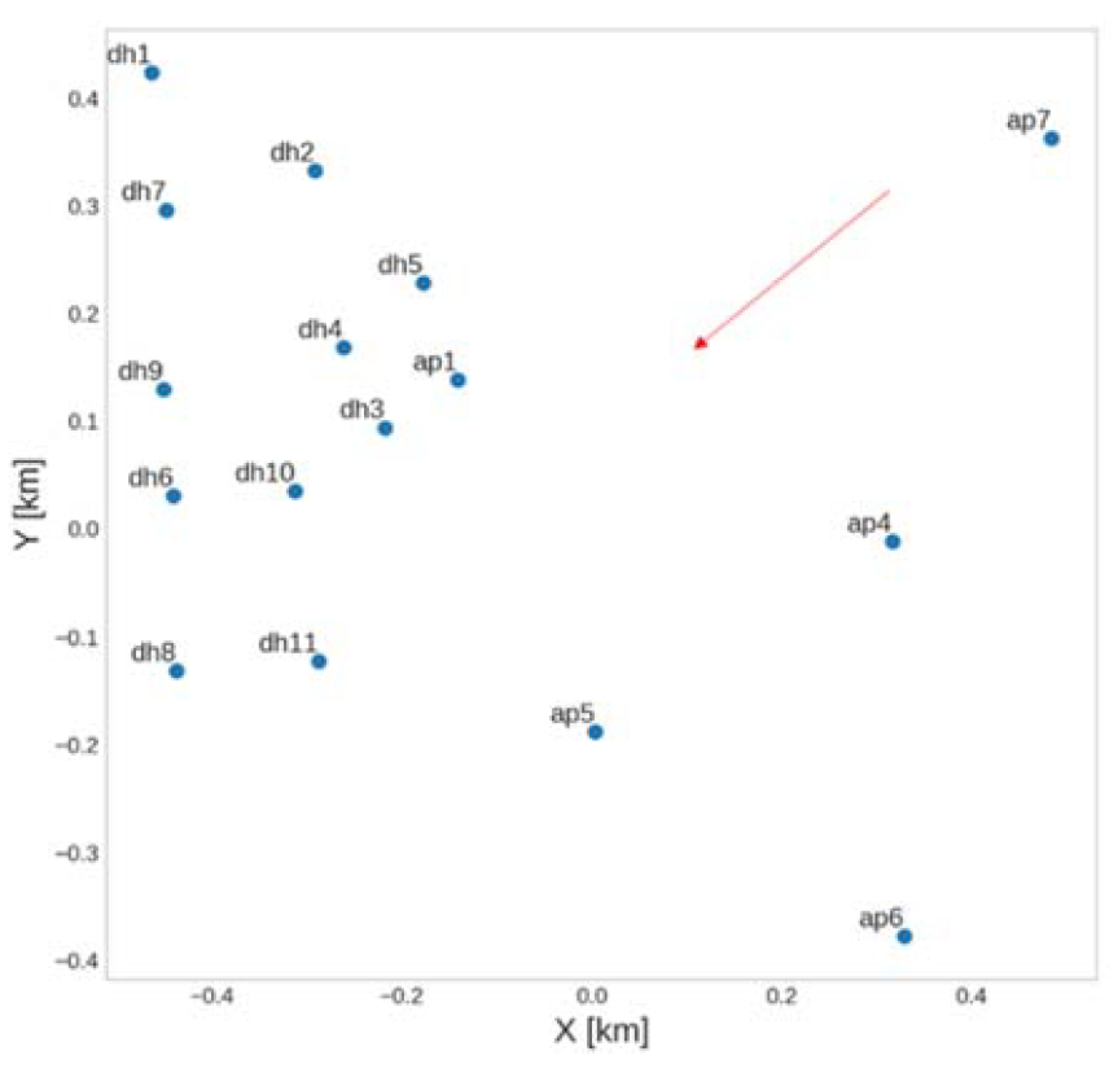
For the study, publicly available data provided by the National Renewable Energy Laboratory, namely the OIH dataset [3], were selected. The dataset is formed by seventeen irradiance sensors (named from here on, measuring locations) located on the Oahu Island of Hawaii, with one square kilometre of spatial resolution (as shown in Figure 1) and provides a high density for the analysis to be carried out. The time resolution for measuring the GHI is one second (from March 2010 to October 2011). The data were measured in a region with known prevailing winds from the east and predominantly the northeast.

In the initial analysis of the data, the information from the ap3 measuring location was removed due to missing data; only the information from the remaining sixteen measuring locations was used. As part of the pre-processing of the data, the data were resampled to ten seconds; the night hours were removed based on a solar elevation angle with a threshold of 5° (to keep sunrise and sunset information). The GHI time series was normalised using the clearness index (calculated with k(t) = GHI/I₀, where I₀ is the extraterrestrial irradiance on the horizontal surface, at a t moment).

As for the ML models considered, three popular algorithms were selected as follows: (1) the RF regression model [4] forms a combination of predictor trees, the prediction delivered being formed by taking the mean of k trees; (2) the XGBoost model [5] is the implementation of the gradient boosting decision tree model that creates the trees sequentially, allowing learning from errors in the previous step (unlike RF, which creates the trees in parallel); and (3) the LightGBM model [6] is an optimisation of the XGBoost model that speeds up the training time by almost twenty times with similar accuracy levels. Therefore, the RF model is an example of a bagging ensemble model, while XGBoost is a boosting ensemble model. LightGBM is an optimisation of the XGBoost model with almost the same degree of certainty in its predictions.

As for the experimental design, an analysis of the influence of including the zonal component and meridional component was performed. The zonal component, referred to as $u$, is the horizontal velocity component along a circle of latitude in a west to east direction, and the meridional component, referred to as $v$, is the horizontal velocity component along a meridian from south to north. The problem can be defined as follows: multiple GHI series $\left\{G^1,\cdots ,G^d\right\}$, where $d$ is the number of irradiance measuring locations, and each $G$ represents a time series from specific measuring locations; the model inputs are registries from the OIH dataset as $\left\{G_p\left(t-l\right),u,v\right\}$;$l$represents the number of lags, $l\in \left\{1,\cdots ,n\right\}$, $p$ is the number of series, $p\in \left\{1,\cdots ,d\right\}$, $u$ is the zonal component, $v$ represents the meridional component, while $G_{k^{\left(t\right)}}$ is the target of the model for the $k^{th}$ measuring location.

The considered models were implemented in the scikit-learn library [7] and trained using the “GridSearch cross validation” function. During training, the hyperparameters optimised for XGBoost and LightGBM were the learning rate, $lr$; $lr\in \left[0.001,0.01,0.1,0.15,0.3,0.45\right]$, and the maximum depth, $md$; $md\in \left[5,10,15,20,25\right]$, with the optimised $lr$ being 0.1 and 10 and the optimised $md$ being 0.1 and 15 for XGBoost and LightGBM, respectively. The considered hyperparameters for RF were the minimum number of leaves, $nl$, and the number of estimators, $ne$; $nl$, $ne\in \left[100,150,200,250,300\right]$, with the optimised $nl$, $ne$ values being 0.01 and 150, respectively. All models were trained using the spatiotemporal approach (considering the lags of the neighbours) in two training scenarios (where the wind components are provided, and vice versa). The performance of the models trained with and without the inclusion of wind variables was evaluated with popular performance metrics applied to assess the accuracy of the regression models, namely, the mean absolute error (MAE), the root mean squared error (RMSE), and the forecast skill (FS) score.

3. Results and Discussion

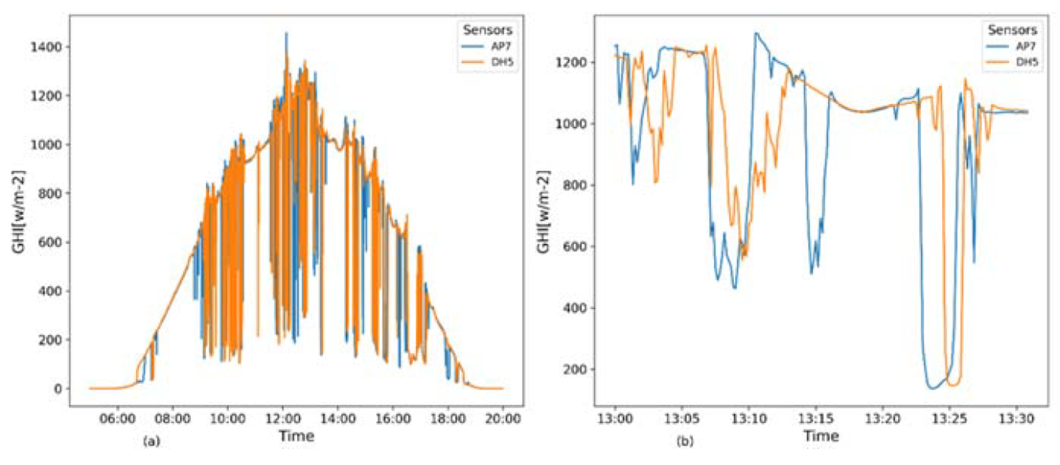
We start with an analysis of the variability being captured and then show the results obtained by the three algorithms. In Figure 2, an example of the spatial and temporal context of the solar variability shows that, when two locations are taken on a given cloudy day, the observed GHI values can vary greatly with changes in the sun’s geometry and cloud movement.

A comparison of the evaluated metrics obtained by the considered ML models is presented in

Table 1. Mean performance metrics obtained by the models trained using the spatiotemporal approach for all measuring locations (grouped by the inclusion of wind data information).

	Wind Variables Considered			No Wind Variables Considered
Model	MAE (W/m2)	RMSE (W/m2)	FS Score (%)	MAE (W/m2)	RMSE (W/m2)	FS Score (%)
RF	27.46	70.13	12.07	29.19	71.32	10.57
LightGBM	22.03	58.60	26.50	23.05	59.41	25.49
XGBoost	20.63	57.70	27.63	21.20	58.31	26.87

. It can be observed that all models evaluated improved their FS score with the inclusion of wind components. XGBoost was the best performer, with an average FS score of 27.63% for all measuring locations. LightGBM achieved an average FS score of 26.50%, while RF obtained an average FS value of 12.07%.

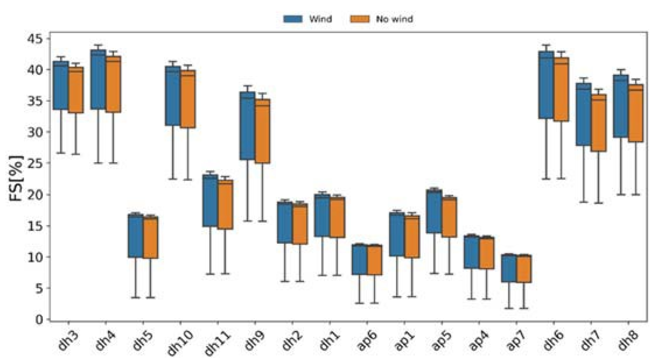
As found in Figure 3, the measuring locations with the highest FS scores are those that have the largest number of neighbours in the direction of the wind. In the ap7, ap4, and ap5 measuring locations, wind variables had less influence on the outcome and featured the lowest FS values. In the dh3, dh4, dh6, and dh10 measuring locations, the results were further improved by the introduction of wind components and displayed the best FS scores. The experiments demonstrate that the inclusion of wind components can improve the prediction results.

4. Conclusions

In this work, the influence of introducing the zonal and meridional wind components as input variables for the ML models was analysed. The study employed three tree-based algorithms for solar radiation forecast, using on OIH dataset trained using a spatiotemporal approach by including lags from neighbouring measuring stations in scenarios where wind and no wind data were used as input. The results demonstrate that using the wind components as input variables delivered an average improvement of approximately 1% in the FS value over the training scenario without wind data.

This implies that, although wind data are not highly correlated with solar radiation, they can indicate cloud movement and other atmospheric conditions and become an effective predictor of solar radiation. For future research, (1) fewer characteristics could be studied by including only the lags of neighbours in the predominant wind direction, and (2) more complex models such as those provided by deep learning implementation should be considered.