Next Article in Journal
Agricultural Cultural Landscapes in America and Their Cartographic Delimitations
Previous Article in Journal
Evaluation of Interpolation Methods for Refractivity Mitigation
 
 
environsciproc-logo
Article Menu

Article Menu

Please note that, as of 4 December 2024, Environmental Sciences Proceedings has been renamed to Environmental and Earth Sciences Proceedings and is now published here.
Proceeding Paper

A Linear Regression Model for Live Fuel Moisture Content Estimation during the Fire Season in Shrub Areas of the Province of Valencia in Spain Using Sentinel-2 Remote Sensing Data †

by
Kenneth Pachacama-Vallejo
* and
Ángel Balaguer-Beser
Geo-Enviromental Cartography and Remote Sensing Group (CGAT-UPV), Universitat Politècnica de València, Camí de Vera, s/n, 46022 València, Spain
*
Author to whom correspondence should be addressed.
Presented at the IV Conference on Geomatics Engineering, Madrid, Spain, 6–7 July 2023.
Environ. Sci. Proc. 2023, 28(1), 12; https://doi.org/10.3390/environsciproc2023028012
Published: 25 December 2023
(This article belongs to the Proceedings of IV Conference on Geomatics Engineering)

Abstract

:
Live Fuel Moisture Content (LFMC) describes the amount of water present in any type of vegetation and helps quantify the amount of fuel available in a wildfire. In this paper, a multivariate linear regression model was built to estimate the LFMC of the weighted average of all shrub-type species present, using the fraction of canopy cover (FCC) of each forest species as weights. Sample training was conducted with field data obtained during the fire season of the years 2019, 2020 and 2021 in 15 plots of a Mediterranean area where vegetation composed of the shrub-type species dominates. Different spectral indices extracted from Sentinel-2 together with the mean surface temperature, the accumulated precipitation and the seasonal parameters were considered as predictors. The results were compared with the extrapolation of another model trained with field data collected in the year 2019.

1. Introduction

Live Fuel Moisture Content (LFMC) is the measure of the percentage of water that a plant species contains in relation to its total dry mass and plays a fundamental role in the dynamics that a wildfire can have at its start and development [1]. It is directly related to the amount of energy required to evaporate the water before ignition. Therefore, a high percentage of moisture contained in the vegetation reduces or completely prevents flammability and the consequent spread of fire [2].
Through satellite images, a spatiotemporal monitoring of vegetation cover on the Earth’s surface is possible. These images allow us to analyze the spectral response captured in the portions of bands separated by the wavelength range of the electromagnetic spectrum, which, depending on the type of sensor used, will offer a series of possibilities to describe the LFMC [2].
In the work of Costa-Saura et al. [3], an LFMC estimation model was created using data obtained in the fire season of 2019 in 15 shrub plots in the province of Valencia in Spain, using as predictors a Sentinel-2 spectral index of 10 m of spatial resolution, smoothed by the Savitzky–Golay filter, in addition to a mean surface temperature and a mean wind speed. Later, Arcos et al. [4] proved that a higher accuracy was achieved in the models that used unsmoothed spectral indices and considered an accumulated precipitation variable when using data from two different years (2019 and 2020) in three plots belonging to the study area of [3].
This paper shows an extension of the regression model described in [3] using data obtained from the same 15 plots but in three fire seasons (in the years 2019, 2020 and 2021). Our model uses unsmoothed Sentinel-2 spectral indices as in [4] and replaces the average temperature with a static variable that reflects the periodic behavior introduced together with an accumulated precipitation variable to obtain a model for years with different rainfall regimes.

2. Methods

2.1. Study Area

This research was carried out in the Province of Valencia located to the south-east of the Iberian Peninsula on the Mediterranean coast. Fifteen plots described in [3] where shrub type species dominate were considered. Each plot was defined in a circular area of 30 m in radius where the density and type of vegetation were homogeneous and where samples of existing species were collected.

2.2. Field Data

Biweekly field samples for all species in each plot were collected between the months of June and October of the years 2019, 2020 and 2021. The LFMC for each specie, date and plot was calculated as the percentage of water contained in vegetation on a dry weight basis following Equation (1):
LFMC = W f W d W d · 100
where W f is the fresh weight and W d is the dry weight. To have a single indicator by date for all shrub species in each plot, LFMCWAS (LFMC weighted average in shrubs) was calculated as the weighted average of the LFMC in all the shrub species existing in the plot, using the fraction of canopy cover (FCC) of each one as weights according to Equation (2), where j varies according to the shrub species present in the plot.
LFMC WAS date ,   plot = Σ j LFMC j date ,   plot × FCC j Σ j FCC j

2.3. Spectral Indices, Meteorological Parameters and Static Variables

Three types of spectral indices were considered: first, indices that respond to the photosynthetic activity of vegetation, e.g., Normalized Difference Vegetation (NDVI), Visible Atmospherically Resistant Index (VARI) and Soil Adjusted Vegetation Index (OSAVI); second, indices related to soil and vegetation water content, e.g., Normalized Difference Water Index (NDWI) and Normalized Difference Moisture Index (NDMI); and third, indices related to the greenness of vegetation, e.g., Transformed Chlorophyll Absorption Index (TCARI) and Vegetation Index-Green (VIGreen) [3]; and finally, TCARI_OSAVI = TCARI/OSAVI [3]. Spectral indices were generated from Sentinel-2 satellite imagery, using Google Earth Engine and a spatial resolution of 20 meters, and their value was defined from the mean of the pixels that intersected with a circular buffer of a 30 meter radius centered on each plot. In addition, the average and range of such indices for the period studied in each plot were also calculated. The values registered at the meteorological observatories were interpolated using the Meteoland R package to obtain the accumulated precipitation in the previous 15, 30 and 60 days (p15, p30 and p60) and the mean surface temperature in the 7, 15, 30 and 60 days (t7, t15, t30, t60) prior to each field sample from the years 2019, 2020 and 2021. Other computed indices were the average wind speed in Km/h for 600 s of the maximum daily wind gusts in the previous 7 and 15 days [3]. Variables sin_DOY and cos_DOY were calculated, respectively, as the sine and cosine for the day of the year [1].

2.4. Multivariate Linear Regression Models

A multivariate linear regression model (MLR_19_20_21) was calculated using three years of data and by following the steps described in Figure 1. First, a stepwise forward linear regression was applied using variables described in Section 2.3 as predictors. Second, the selection of a maximum of six predictors was carried out using the Akaike information criterion. And finally, the Variance Inflation Factor (VIF) of predictors in general linear models was calculated to analyze the quality of contribution that the independent variables present to the model. Moreover, the best model (R2adj = 0.70) in Costa-Saura et al. [3] of the year 2019 was replicated with our 2019 data to later extrapolate and compare their adjustability in the years 2020 and 2021.

3. Results and Discussion

Table 1 shows selected variables and fitted coefficients in MLR_19_20_21 and MLR_19 models. The spectral indices used in the first regression model were VARI and TCARI_OSAVI together with two statistics of spectral indices in each plot (mean_VARI and range_NDVI) calculated using all spectral data in the fire season of the three years. A static seasonal parameter (sin_DOY) and an accumulated precipitation variable (p60) helped to describe the LFMCWAS. Furthermore, in the replicated model, the fit and coefficients achieved were very similar to the original [3]. All predictors were statistically significant with VIF parameters below 5, indicative of non-multicollinearity. The adjusted R2 was smaller in the model using the data from all three years due to the inter-annual variability of LFMCWAS. This causes the RMSE and MAE to be higher in the MLR_19_20_21 model, but their values are below 12.
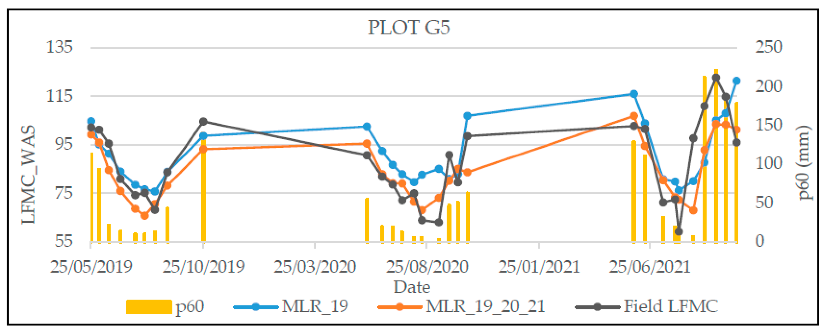
Figure 2 shows LFMCWAS values obtained in plot number 2 described in [3], which coincides with plot G5 given in [4]. Model MLR_19 achieved higher accuracy for the year 2019, but when it was extrapolated to the other years, it lost accuracy due to annual differences, especially in the rainfall regime according to that described by Arcos et al. [4]. The MLR_19_20_21 model estimated values closer to the field values for the years 2020 and 2021 where the minimum values were reached. In addition, the values estimated by MLR_19 at the beginning and at the end of the fire season during the years 2020 and 2021 were higher than those obtained in the field. Figure 2 shows the p60 values obtained in field dates, which indicated the importance of the precipitation variable in the MLR_19_20_21 model, since it fitted better with the minimum and maximum values and more effectively followed the trend of the field LFMCWAS.

4. Conclusions

This paper allowed us to verify that the changes in the precipitation pattern caused LFMCWAS forecast errors when using a regression model obtained with data from previous years. The model obtained with data collected in the fire season for three consecutive years selected as its predictors an accumulated precipitation variable, together with a seasonal parameter that depends on the day of the year, instead of other meteorological variables obtained such as the average temperature or the wind speed. To describe the spatial differences of LFMCWAS between plots, temporal averages of the spectral indices obtained in each plot had to be used together with the range (the difference between the maximum and minimum), calculated using all possible dates in our study period, so they only varied at the spatial level. In addition, vegetation indices predominate over water content spectral indices.

Author Contributions

Conceptualization, K.P.-V and Á.B.-B.; methodology, K.P.-V and Á.B.-B.; software, K.P.-V and Á.B.-B.; validation, K.P.-V and Á.B.-B.; writing—original draft preparation, K.P.-V and Á.B.-B.; writing—review and editing, K.P.-V and Á.B.-B. All authors have read and agreed to the published version of the manuscript.

Funding

This research was founded by a collaboration agreement between the company Red Eléctrica de España and the Universitat Politècnica de València (2020–2023), as well as the research project PID2020-117808RB-C21 funded by MCIN/AEI/10.13039/501100011033 and by ESF Investing in your future.

Data Availability Statement

Sentinel-2 data are freely available. The in situ LFMC and meteorological data were obtained from the Valencian regional government under specific research agreement.

Acknowledgments

The authors thank the VAERSA enterprise and the Direcció General de Prevenció d’Incendis Forestals of the Generalitat Valenciana for providing the LFMC measurement data in the field and the meteorological data through the AEMET. The authors thank María Alicia Arcos-Villacís for providing interpolated meteorological data and for their suggestions.

Conflicts of Interest

The authors declare no conflicts of interest.

References

  1. Cunill Camprubí, À.; González-Moreno, P.; Resco de Dios, V. Live Fuel Moisture Content Mapping in the Mediterranean Basin Using Random Forests and Combining MODIS Spectral and Thermal Data. Remote Sens. 2022, 14, 3162. [Google Scholar] [CrossRef]
  2. Yebra, M.; Quan, X.; Riaño, D.; Larraondo, P.R.; van Dijk, A.I.; Cary, G.J. A fuel moisture content and flammability monitoring methodology for continental Australia based on optical remote sensing. Remote Sens. Environ. 2018, 212, 260–272. [Google Scholar] [CrossRef]
  3. Costa-Saura, J.M.; Balaguer-Beser, Á.; Ruiz, L.A.; Pardo-Pascual, J.E.; Soriano-Sancho, J.L. Empirical Models for Spatio-Temporal Live Fuel Moisture Content Estimation in Mixed Mediterranean Vegetation Areas Using Sentinel-2 Indices and Meteorological Data. Remote Sens. 2021, 13, 3726. [Google Scholar] [CrossRef]
  4. Arcos, M.A.; Balaguer-Beser, Á.; Ruiz, L.Á. Modelos Empíricos De Predicción Del Contenido De Humedad Del Combustible Vivo Mediante Índices Espectrales De Sentinel-2 Y Datos Meteorológicos. In Proceedings of the 3rd Congress in Geomatics Engineering, Valencia, Spain, 7–8 July 2021. [Google Scholar] [CrossRef]
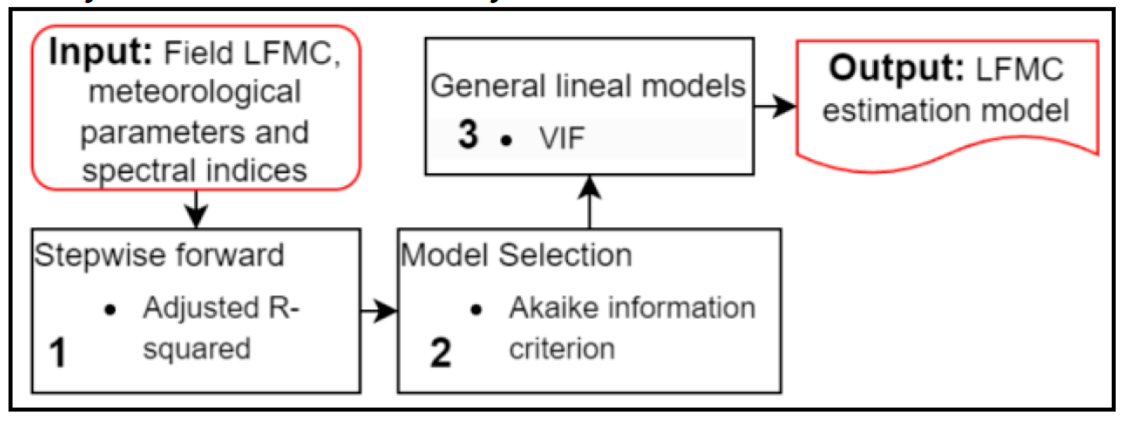
Figure 1. Multivariate linear regression process used to estimate the LFMC.
Environsciproc 28 00012 g001
Figure 2. LFMCWAS values estimated on the dates of sampling in the field in plot number 2, described in [3] (G5 in [4]), using MLR_19_20_21 and MLR_19 models, the coefficients of which are given in Table 1. Field LFMC corresponds to the measured data used to calibrate regression models and p60 corresponds to the accumulated precipitation in the last 60 days.
Environsciproc 28 00012 g002
Table 1. Multivariate linear regression models for LFMCWAS defined by (2) in shrubs. The columns represent the name of model and variables, coefficients, p-value of each coefficient, variance inflation factor (VIF), adjusted R2 (R2adj), root mean square error (RMSE) and mean absolute error (MAE).
ModelVariableCoefficientp-ValuesVIFR2adjRMSEMAE
MLR_19_20_21Intercept124.222 0.51911.138.54
sin_DOY−12.3636<0.001.18564
p600.066198<0.001.34219
TCARI_OSAVI−93.5614<0.001.70399
VARI110.723<0.003.24571
Mean_VARI−120.596<0.002.97184
Range_NDVI−44.4529<0.001.08075
MLR_19 *Intercept191.091 0.658 *8.83 *6.52 *
t60−2.55324<0.001.35301
NDMI153.357<0.003.39691
Mean_NDMI−91.90450.00013.31885
W7−4.72606<0.001.16423
* Only data from the year 2019 was used to replicate the model and its consequent statistics.
Disclaimer/Publisher’s Note: The statements, opinions and data contained in all publications are solely those of the individual author(s) and contributor(s) and not of MDPI and/or the editor(s). MDPI and/or the editor(s) disclaim responsibility for any injury to people or property resulting from any ideas, methods, instructions or products referred to in the content.