1. Introduction
Signals traveling through the atmosphere are affected in different ways, such as the effect of refraction along the signal path. Atmospheric refraction affects all geomatic techniques (electronic distance measurement (EDM), total station (TS), terrestrial laser scanner (TLS), image, levelling, etc.) [
1,
2]. Assuming measurements are made with a relative precision of 1ppm, this effect can be only neglected for short distances, i.e., lower than 200 m. However, for medium or long distances, where accuracy is critical (as in the case of deformation monitoring), it is crucial to eliminate or mitigate the effect of refraction. In these cases, neglecting the effect of atmospheric refraction can lead to erroneous results, for example, when comparing two point clouds acquired by TLS, coordinate differences up to decimeters caused by refraction under different atmospheric conditions can be erroneously detected as deformations [
2].
Different approaches to mitigate refraction can be found in the literature [
3,
4]. For this study, a meteorological sensor network deployed in the geodetic network of Cortes de Pallás [
5,
6] is used to explore the possibility of interpolating refractivity to obtain a 3D model that can be applied to different geomatic techniques.
Refractivity depends on meteorological parameters, including temperature, pressure, and humidity [
7]. Several studies have tested methods for temperature interpolation [
8,
9], but other parameters such as humidity are more complicated to model due to their high local variability. For this reason, interpolating refractivity instead of meteorological parameters is a more convenient approach.
In this paper, Inverse Distance Weighting (IDW) interpolation (both 2D and 3D) and Multiple Linear Regression (MLR) are applied to a nine-station network in Cortes de Pallás (Spain) for a period of about 8 hours. The results of the models are analyzed in terms of root-mean-square error (RMSE). The next section of this paper shows the theoretical basis of the refractivity calculation, interpolation methods, and model evaluation. The data used are also described. Then, the results are presented, and finally, some conclusions are drawn in the last section.
2. Data and Methods
2.1. Refractivity Calculation
The refractive index for a specific medium (
) is defined as the ratio of the speed of the propagation of an electromagnetic wave in vacuum to that in medium. Its value for air is very close to one, so, usually, the refractivity
N defined as
is used instead.
Refractivity is calculated from meteorological parameters, and its expression depends on the signal wavelength. Visible and infrared, for EDM to within 1 ppm, is calculated as [
7]:
where
is the temperature (in K),
is the total pressure (in hPa),
is the partial water pressure (in hPa), and
is the group refractivity.
The group refractivity in Equation (1) is obtained as:
with
being the carrier wavelength of the EDM in µm. In this study, the value of the Leica TM-30 TS is used (0.658 µm) as it has been used to monitor the zone in the different field campaigns.
2.2. Interpolation Methods
There exist a great number of interpolation algorithms for different purposes. In fields such as geography or meteorology, some commonly used are Kriging, co-kriging, and IDW [
8,
9].
Some of them have been tested and discarded for the data of this study, for instance, the Kriging method [
8]. This method is based on the premise that the spatial variation continues with the same homogeneous pattern, so a function can be fitted to the semivariogram. However, this does not occur in our data. The semivariogram obtained cannot be adjusted because the premise of homogeneous spatial variation is not true. On the other hand, the Inverse Distance Weighting (IDW) method and Multiple Linear Regression (MLR) can be used as follows:
This estimates values by averaging the ones of the sample data points. The closer a point is to the point where the value is being estimated, the more influence or weight it will have in the averaging process.
Several types of distances can be used (Euclidean, Manhattan, etc.). Despite some other options having been tested, in this study, only the Euclidean distance (both 2D and 3D) is used.
This allows for the generation of a linear model in which the value of the dependent variable is determined from a set of independent variables. In this case, the variable to be determined is refractivity N, and the input variables are 3D point coordinates.
The general expression for MLR is [
9]:
2.3. Model Evaluation
The different models have been evaluated by means of the root-mean-square error (RMSE) obtained using cross-validation. For cross-validation, the model is generated for
n-1 stations, and the excluded station is then used to calculate the error. The RMSE is then obtained as:
where
is the number of stations,
the calculated value, and
is the obtained value by the model.
2.4. Data
The data used in this study were acquired during a field campaign in Cortes the Pallás. We installed nine data loggers in different stations, so meteorological parameters (temperature, pressure, and relative humidity) were automatically stored every minute.
Table 1 shows the coordinates of the stations used in this study (Easting (E), Northing (N) corresponds to UTM coordinates zone 30, and H is the orthometric height). These stations are periodically monitored by Universitat Politècnica de València (UPV) [
5].
3. Results
3.1. Model Correctness
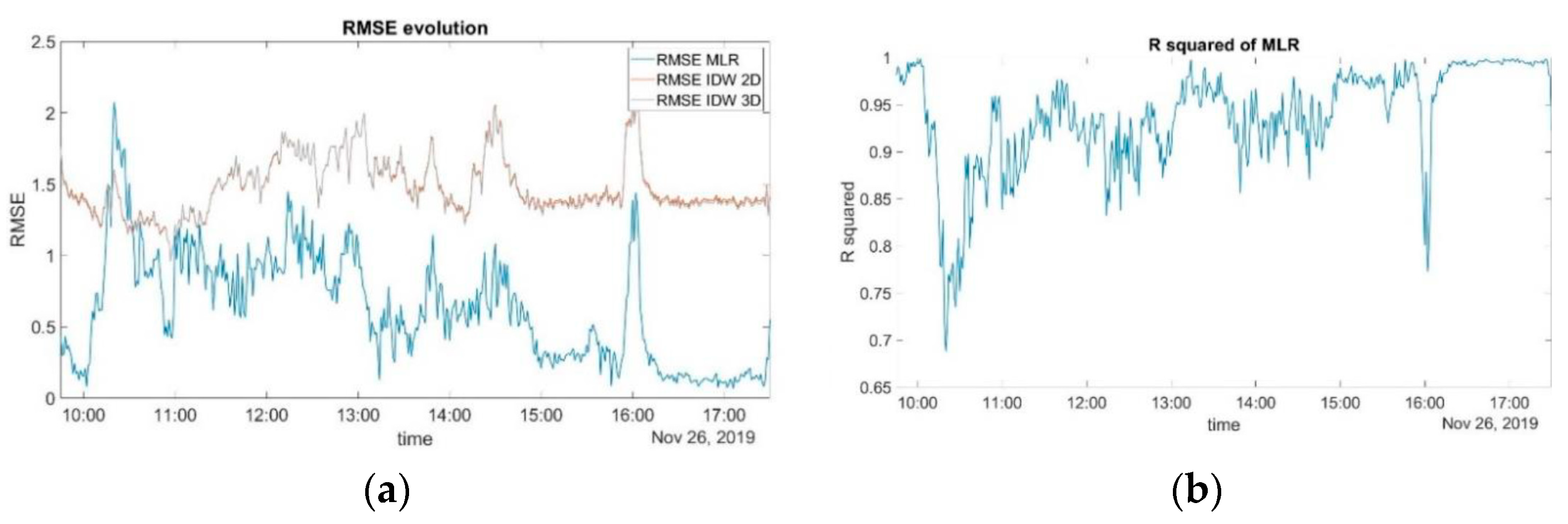
Three different models (IDW 2D, IDW 3D, and MLR) were obtained for each epoch (that is every minute). The RMSE with cross-validation was also obtained epoch by epoch.
Figure 1a shows the evolution of the RMSE of refractivity obtained with each model during the observation period.
Figure 1b shows the coefficient of determination R
2, for the MLR model, as this is the one that performs better in terms of RMSE.
3.2. Interpolated Refractivity
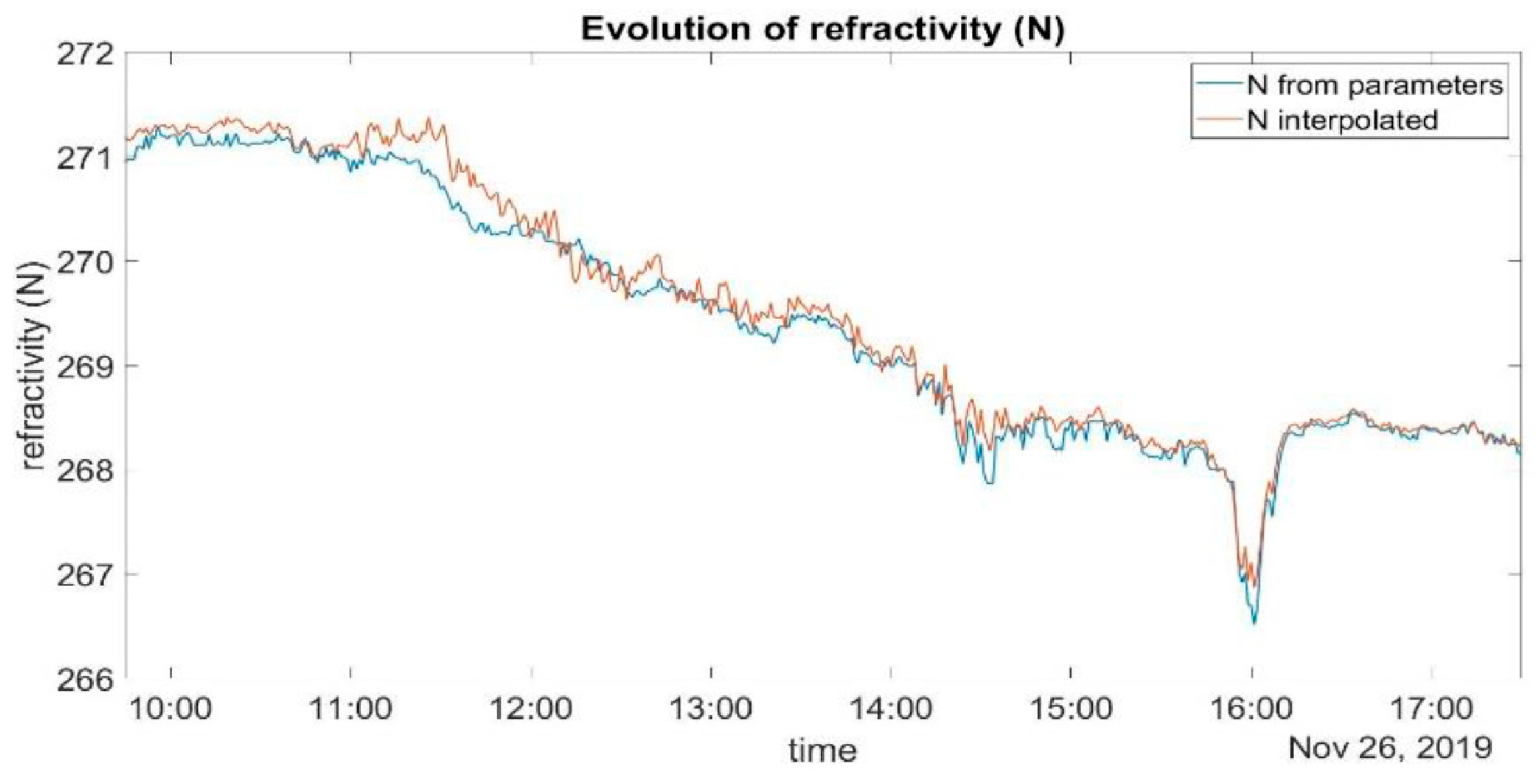
Following cross-validation with a model generated by excluding one station, both real and calculated refractivity can be graphically displayed. As an example,
Figure 2 shows the evolution of refractivity N at station 8006. Refractivity tends to decrease during observation hours. This change is mainly due to temperature changes during the day. Around 16:00 p.m., refractivity suddenly decreases with a peak in the obtained RMSE and R
2 (
Figure 1).
4. Conclusions
IDW interpolation shows similar behavior using 2D or 3D coordinates, and the value obtained for the refractivity RMSE is higher than the one obtained using MLR. MLR performs better in terms of RMSE, with a value under one (dimensionless) at most epochs. In terms of R2, MLR models have values above 0.85 in most epochs.
In the worst case, the model shows an RMSE of around 2 and R2 of 0.7. When raw meteorological data are used, no smoothing is applied, so an error in any of the stations can lead to outliers. Meteorological data smoothing could be studied in future works.
The evolution of real refractivity and refractivity calculated with MLR shows good agreement. This, along with the RMSE and R2 of the MLR models, indicates that this method is highly applicable to potentially mitigate atmospheric refraction in mountainous areas such as Cortes de Pallás.
Due to the harsh orography of the area, the local variability of meteorological parameters, and the critical precision required to prevent rockfalls, more research seems necessary. For future works, the model is pretended to be refined by adding gradient information or using additional data as the atmospheric information provided by GNSS techniques.
Author Contributions
Conceptualization and methodology, R.L., L.G.-A. and S.B.; software, R.L.; validation, R.L., L.G.-A. and S.B.; writing—original draft preparation, R.L.; writing—review and editing and funding acquisition, L.G.-A. and S.B. All authors have read and agreed to the published version of the manuscript.
Funding
We acknowledge the Programa de Ayudas de Investigación y Desarrollo (PAID- 01-20) de la Universitat Politècnica de València for funding the research contract of Raquel Luján.
Institutional Review Board Statement
Not applicable.
Informed Consent Statement
Not applicable.
Data Availability Statement
The data can be obtained from the corresponding author on request.
Conflicts of Interest
The authors declare no conflict of interest.
References
- Zhou, J.; Shi, B.; Liu, G.; Ju, S. Accuracy analysis of dam deformation monitoring and correction of refraction with robotic total station. PLoS ONE 2021, 16, e0251281. [Google Scholar] [CrossRef] [PubMed]
- Friedli, E.; Presl, R.; Wieser, A. Influence of atmospheric refraction on terrestrial laser scanning at long range. In Proceedings of the 4th Joint International Symposium on Deformation Monitoring (JISDM), Athens, Greece, 15–17 May 2019. [Google Scholar]
- Rodriguez, F.A.C.; Veiga, L.A.K.; Soares, W.A. Temperature Acquisition System for Real Time Application of First Velocity Correction by EDM (Electronic Distance Measurement). Geoplanning: J. Geomatics Plan. 2021, 8, 61–74. [Google Scholar] [CrossRef]
- Hirt, C.; Guillaume, S.; Wisbar, A.; Bürki, B.; Sternberg, H. Monitoring of the refraction coefficient in the lower atmosphere using a controlled setup of simultaneous reciprocal vertical angle measurements. J. Geophys. Res. Atmos. 2010, 115. [Google Scholar] [CrossRef]
- García-Asenjo, L.; Martínez, L.; Baselga, S.; Garrigues, P.; Luján, R. Design, establishment, analysis, and quality control of a high-precision reference frame in Cortes de Pallás (Spain). Appl Geomat 2023, 15, 359–370. [Google Scholar] [CrossRef]
- García-Asenjo, L.; Martínez, L.; Baselga, S.; Garrigues, P. Establishment of a multi-purpose 3D geodetic reference frame for deformation monitoring in Cortes de Pallas (Spain). In Proceedings of the 4th Joint International Symposium on Deformation Monitoring (JISDM), Athens, Greece, 15–17 May 2019. [Google Scholar]
- International Union of Geodesy and Geophysics (IUGG). Resolution 3 of the International Association of Geodesy. In Proceedings of the Comptes Rendus of the XXII General Assembly, Birmingham, UK, 19–30 July 1999.
- Vicente-Serrano, S.M.; Saz-Sánchez, M.A.; Cuadrat, J.M. Comparative analysis of interpolation methods in the middle Ebro Valley (Spain): Application to annual precipitation and temperature. Clim. Res. 2003, 24, 161–180. [Google Scholar] [CrossRef]
- Kayıkçı, E.T.; Kazancı, S.Z. Comparison of regression-based and combined versions of Inverse Distance Weighted methods for spatial interpolation of daily mean temperature data. Arab. J. Geosci. 2016, 9, 690. [Google Scholar] [CrossRef]
| Disclaimer/Publisher’s Note: The statements, opinions and data contained in all publications are solely those of the individual author(s) and contributor(s) and not of MDPI and/or the editor(s). MDPI and/or the editor(s) disclaim responsibility for any injury to people or property resulting from any ideas, methods, instructions or products referred to in the content. |
© 2023 by the authors. Licensee MDPI, Basel, Switzerland. This article is an open access article distributed under the terms and conditions of the Creative Commons Attribution (CC BY) license (https://creativecommons.org/licenses/by/4.0/).


