Methods of Identification Coherent Structures in Atmospheric Numerical Data ^†

Abstract

Coherent structures (CS), or vortices, are playing an important role in Earth’s climate system, since they are responsible for a significant part in the momentum, heat, mass, etc., transportation of any fluid, including the atmosphere and the ocean. This is true for all scales of motion, but it is especially important for more chaotic mesoscale structures. Automatic identification of CS has the potential to enable automatic categorization of mesoscale vortices and the development of a general mesoscale climatology. Currently, there is no objective definition of a vortex, mainly due to difficulties in determining its outer boundary. Despite this challenge, recent developments in atmospheric turbulent dynamics have attempted to address this issue. In this study, we examined the implementation of three most popular Eulerian methods for identifying CSs in mesoscale-resolving gridded data. Our primary objective was to determine the most effective method for vortex identification on a scale relevant to Earth science data.

1. Introduction

Coherent structures (CS), which are heavily associated with vortices, are critical to understanding the dynamics of the ocean and atmosphere at all scales. At synoptic and mesoscales, vortices are involved in the transfer of momentum, temperature, and mass in both the ocean and atmosphere. Therefore, accurate CSs identification is crucial to improving our understanding of geophysical processes and their dynamics. Moreover, the accuracy of these dynamics heavily relies on the objectivity of vortex identification.

Over the past 50 years, numerous attempts have been made to develop an objective criterion for identifying vortices. Various approaches can be categorized into two primary groups: Eulerian and Lagrangian. The Eulerian approach relies on topological analysis of dynamic variable fields, while the Lagrangian approach examines individual fluid particle trajectories using dynamical systems theory methods.

The challenge of objective CS identification lies in the absence of a universally accepted mathematical definition for a vortex, particularly its outer boundary. For large-scale motions, this issue is partially addressed by defining a cyclone’s boundary by its last closed isobar. While some progress has been made in solving the problem of vortex identification in specific cases, a general approach to defining vortices remains unsolved.

The primary objective of this research is to take the first step in building a global climatology of mesoscale dynamics. To achieve this goal, we first need to develop a reliable method for identifying vortices. In this paper, we investigate Eulerian approach criteria to gain the basic statistics of CSs, as methods from this group are more popular and less computationally demanding. Primarily, these criteria are employed to identify microscale turbulence. Eulerian methods detect CSs locally, utilizing topology analysis of instantaneous fields of scalar values. The most popular Eulerian criteria are based on velocity gradient tensor $\nabla \overrightarrow{u}$ analysis.

Historically, the Q-criterion [1], which employs velocity gradient tensor decomposition into symmetric and antisymmetric parts, was the first 3D vortex criterion. It was derived under the assumption of incompressible flow, with a vortex defined as a region with a positive second invariant of $\nabla \overrightarrow{u}$. The Q-criterion is frequently applied to turbulent flows, and its 2D-version (Okubo–Weiss criterion [2,3]) has been widely used in oceanography.

Lugt [4] defined a vortex as “a set of material particles that rotate around a common center” and suggested using closed or spiral flow lines to detect vortices. However, flow lines are not Galilean invariants; hence, Perry and colleagues [5] identified the vortex area as a region with complex eigenvalues c resulting in the Δ-criterion [6].

The ${\lambda }_2$-criterion [7], like the two aforementioned criteria, is based on velocity gradient tensor decomposition but also requires the presence of a local pressure minimum. This criterion was derived from dynamical considerations.

The relevance of this problem is underscored by the development of various Eulerian criteria over the past 30 years. Some criteria involve $\nabla \overrightarrow{u}$ decompositions of higher order (third and above), while others analyze the topology of different hydrodynamic fields. Despite producing similar qualitative results, the CS geometry identified by different methods can vary. In this paper, we examined the applicability of the above-mentioned three widely used criteria for identifying coherent structures in numerical data. We employed atmospheric numerical data, specifically a 40-year 3D hindcast of the North Atlantic atmosphere, North Atlantic Atmospheric Downscaling (NAAD) [8], which will be described in Section 2.2.

2. Materials and Methods

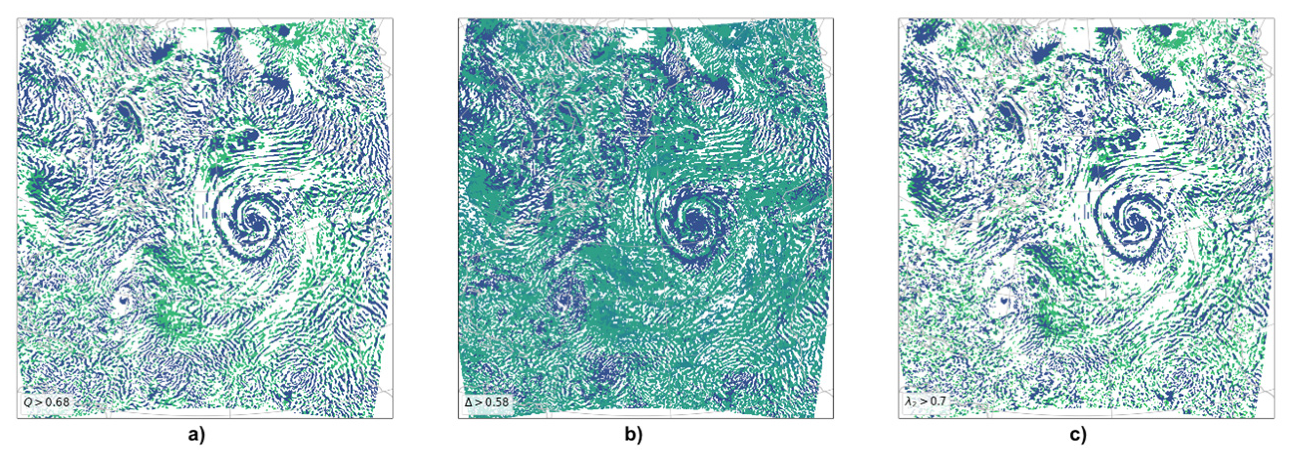
2.1. Basic Vortex Identification Criteria

As mentioned in Section 1, there is a wide variety of coherent structure identification methods. However, the most widely used criteria are the $Q$, $\mathsf{\Delta }$, and ${\lambda }_2$ criteria. In this research, we will examine the applicability of these methods. All of them belong to the Eulerian approach, assuming incompressibility and stationarity of the flow. They are based on the decomposition of the velocity gradient tensor ($\nabla \overrightarrow{u}$) into symmetric and antisymmetric components:

$$\nabla \overrightarrow{u}=\overrightarrow{S}+\overrightarrow{\Omega },$$

(1)

where the symmetric part $\overrightarrow{S}$ represents the velocity deformation tensor, and the antisymmetric part $\overrightarrow{\Omega }$ corresponds to the vorticity tensor. We will employ the Einstein summation rule, where $i,j=1, 2, 3$ is a coordinate system.

The characteristic equation for $\nabla \overrightarrow{u}$ is:

$${\lambda }^3+P{\lambda }^2+Q\lambda +R=0,$$

(2)

where $P$, $Q$, and $R$ denote the three invariants of the $\nabla \overrightarrow{u}$ tensor. We can express them as follows:

$$\begin{array}{c}P=-\left(\nabla \overrightarrow{u}\right),\\ Q=\frac{1}{2}\left({\left(\nabla \overrightarrow{u}\right)}^2-\left(\nabla {\overrightarrow{u}}^2\right)\right)=\frac{1}{2}\left(\parallel \overrightarrow{\Omega }{\parallel }^2-\parallel \overrightarrow{S}{\parallel }^2\right),\\ R=-\det \left(\nabla \overrightarrow{u}\right).\end{array}$$

(3)

2.1.1. Q-Criterion

This criterion characterizes CSs as flow regions where the second invariant $Q$ > 0. This condition implies that the Euclidean norm of the vorticity tensor surpasses the velocity deformation one [1]. Consequently, the $Q$-criterion is defined as follows:

$$Q=\frac{1}{2}\left(\parallel \overrightarrow{\Omega }{\parallel }^2-\parallel \overrightarrow{S}{\parallel }^2\right)>0.$$

(4)

2.1.2. Δ-Criterion

The $\mathsf{\Delta }$-criterion identifies vortices as regions where streamlines exhibit spiral or closed boundaries in the local reference system [9]. To fulfill this condition, the eigenvalues of $\nabla \overrightarrow{u}$ must be complex. To satisfy this condition, the discriminant should be greater than zero:

$$\mathsf{\Delta }={\frac{Q}{3}}^3+{\frac{R}{2}}^2>0.$$

(5)

Upon comparing Equations (4) and (5), it becomes evident that the condition Q > 0 is more stringent than $\mathsf{\Delta }>0$.

2.1.3. ${\lambda }_2$-Criterion

The ${\lambda }_2$-criterion for vortex identification is grounded in a dynamical consideration [7]—vortex existence necessitates a pressure extremum in the plane perpendicular to the vortex axis. To derive the final formula, we begin with the gradient of the Navier–Stokes equation:

$$a_{i,j}=-\frac{1}{\rho }{p}_{,ij}+\nu u_{i,jkk},$$

(6)

where $a_{i,j}$ represents the acceleration gradient, and $p_{,ij}=\nabla {\left(\nabla p\right)}_{ij}={\partial }^{2}p/\partial x_i\partial x_j$ denotes the symmetric pressure Hessian. Subsequently, $a_{i,j}$ can be decomposed into symmetric and antisymmetric components. The symmetric component of (6) is given by:

$$\frac{D{S}_{ij}}{Dt}-\nu S_{ij,kk}+{\Omega }_{ik}{\Omega }_{kj}+S_{ik}{S}_{kj}=-\frac{1}{\rho }{p}_{,ij}.$$

(7)

To satisfy the local minimum condition, the pressure Hessian must have two positive eigenvalues. At this stage, the influence of unsteady non-vortex deformation and viscosity effects is not examined. The final equation is:

$${\overrightarrow{\Omega }}^2+{\overrightarrow{S}}^2=-\frac{1}{\rho }{p}_{,ij}.$$

(8)

Considering the symmetry of the tensor ${\overrightarrow{\Omega }}^2+{\overrightarrow{S}}^2$, it should only possess real eigenvalues (${\lambda }_1$, ${\lambda }_2$ and ${\lambda }_3$). If we sort them like ${\lambda }_1\ge {\lambda }_2\ge {\lambda }_3$, the vortex condition will be:

$${\lambda }_2<0.$$

(9)

Although these three criteria were initially developed for 3D flows, their application in 2D cases yields equivalent results.

2.2. Data

Methods for identifying coherent structures are primarily used in turbulent hydrodynamics. Consequently, to assess their applicability to geophysical data, we will examine data with varying spatial resolutions. Although these methods have the potential to be applied to any medium, we chose to focus on atmospheric data due to the absence of complex geometry in reservoir boundaries, which significantly simplifies calculations.

The North Atlantic Atmospheric Downscaling (NAAD) dataset was created by the Institute of Oceanology RAS. It was based on a non-hydrostatic numerical model of the atmosphere WRF-ARW [10], with a spatial resolution of 14 (HiRes) and 77 km (LoRes), both with 50 vertical levels. For a more detailed description of the model configuration and validation of the results, please refer to paper [8].

2.3. Data Processing

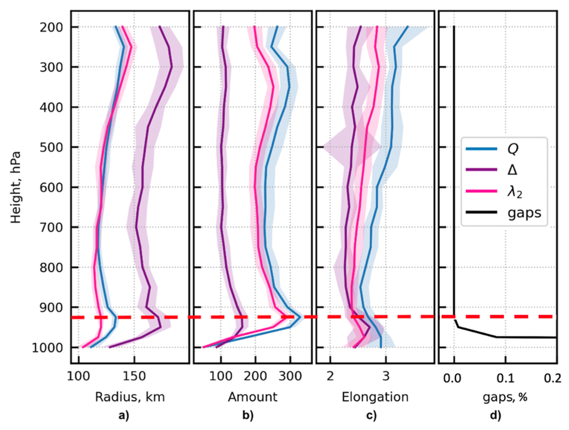
All three criteria ($Q$, $\mathsf{\Delta }$, and ${\lambda }_2$) were applied to the NAAD HiRes data, for which the grid step was 14 km, which potentially enabled mesoscale vortices with an approximate length 70+ km to be resolved. In Figure 1, the results of three normalized criteria at an altitude of about 5.5 km (500 hPa) are given. This height corresponds to free atmosphere height, where the effect of friction on the surface is not significant and CS identification methods should work more adequately. All points satisfying the condition of a coherent structure are indicated by color. It can be observed that the $\mathsf{\Delta }$-criterion field (Figure 1b) appeared more “noisy”, which corroborates the assertion that the $Q>0$ condition is stricter than $\mathsf{\Delta }>0$. Moreover, the strict vortex condition (e.g., ${\lambda }_2>0$) was determined to be too sensitive, highlighting vast areas of CSs that merged with each other (green color). To obtain individual characteristics, it was necessary to change the strict threshold value until the CSs began to stand out clearly (blue color).

Subsequently, the clustering of individual CSs was carried out on each vertical level (Figure 2a). For clustering, horizontal coordinates of points satisfying the threshold value of the criterion were used as a feature description. As a consequence, the method can be easily generalized to the 3D case. Clustering was carried out by the DBSCAN machine learning method (density-based spatial clustering of applications with noise) [11].

Note that Figure 1 shows threshold values for only one height level. However, the threshold value for identifying CSs does not have to be constant though all levels due to differences in vortex dynamics at different levels. In order to check the existence of functional dependence on height, the numbers of isolated CSs, distinguished by DBSCAN at each height level, were calculated and an approximation was made by the values of the maximum gradients of these numbers. Based on this calculation, we decided to use constant threshold value (average over height) in further calculations, as functional dependence was not very notable.

To obtain individual spatial characteristics of each CS, the following method of determining the CS boundary was used. At the first step, the point farthest from the center of the CS belonging to this cluster was determined, and points on a circle of a similar radius with a step of 5 degrees were selected. Then, the CS points closest to the corresponding radial lines were determined. The final boundary is shown in Figure 2b.

After obtaining the CS boundary, geometric characteristics of vortex structures were obtained: centers were determined, areas were calculated, as well as radii assuming the shape of a circle. Moreover, Figure 2b illustrates the superimposed ellipse for the current CS cluster needed to obtain the elongation parameter, which we determined as the ratio of the major and minor semiaxes of an ellipse.

3. Results

According to Section 2.3, we obtained preliminary CS statistics for the summer of 2010 using a 5-day step between fields. This step minimized the synoptic dynamics. Additionally, we used 12:00 UTC times for analysis to ensure consistent atmospheric dynamics throughout the process.

Figure 3a–c illustrates the dependence of the radii, amounts, and elongation of vortex structures on height for the summer seasons. Because the NAAD data were presented at pressure levels, the lowest levels may sink below the surface. As a consequence, missing values appeared in the data (Figure 3d). Thus, when interpreting the results, we relied on data located above 925 hPa.

There is an increasing size (Figure 3a) and decreasing amount (Figure 3b) of CSs as the altitude increases. This trend is consistent with the general understanding of vortex dynamics, as decreasing surface friction leads to less vortex breaking. The second peak in the number of vortices at an altitude of about 8 km was due to the influence of the tropopause. CS elongation (Figure 3c) also showed a slight increase with height due to influence of shear currents of the free atmosphere. Based on elongation distribution, it is worth noting that most of the structures were not symmetrical (close in shape to circles, like tropical cyclones). It should be noted that $Q$- and ${\lambda }_2$-criteria were in good agreement with each other, unlike $\mathsf{\Delta }$-criterion, which reduced the credibility of this method.

4. Discussion

Our study demonstrates that the three most commonly used criteria for identifying coherent structures in microturbulence can also be applied to geophysical data. However, the $\mathsf{\Delta }$-criterion produced noisier results and differed significantly from the other criteria in terms of the vertical distribution of geometric properties of the CSs and other characteristics (which are not shown). This observation raises concerns about the applicability of the $\mathsf{\Delta }$-criterion in geophysical processes. Among the remaining criteria ($Q$ and ${\lambda }_2$), the ${\lambda }_2$-criterion appeared to be the most promising, as it is based on physical concepts.

In general, the Euler approach provides a useful framework for analyzing the main properties of mesoscale structures. However, it has certain limitations. Neglecting the incompressibility and unsteadiness of the flow leads to the use of empirical threshold values instead of strict mathematical conditions ($>0$) for identifying vortex boundaries. This can significantly complicate the search for actual vortex boundaries and lead to uncertainties in the identification of vortices.

References

1. Hunt, J.C.R.; Wray, A.A.; Moin, P. Eddies, Streams, and Convergence Zones in Turbulent Flows; Center for Turbulence Research, Proceedings of the Summer Program: Washington, DC, USA, 1988; pp. 193–208. [Google Scholar]
2. Okubo, A. Horizontal dispersion of floatable particles in the vicinity of velocity singularities such as convergences. Deep-Sea Res. Oceanogr. Abstr. 1970, 17, 445–454. [Google Scholar] [CrossRef]
3. Weiss, J. The dynamics of enstrophy transfer in two-dimensional hydrodynamics. Phys. D Nonlinear Phenom. 1991, 48, 273–294. [Google Scholar] [CrossRef]
4. Lugt, H.J. The Dilemma of Defining a Vortex. In Recent Developments in Theoretical and Experimental Fluid Mechanics; Springer: Berlin/Heidelberg, Germany, 1979; pp. 309–321. [Google Scholar]
5. Perry, A.E.; Chong, M.S. A description of eddying motions and flow patterns using critical-point concepts. Annu. Rev. Fluid Mech. 1987, 19, 125–155. [Google Scholar] [CrossRef]
6. Chong, M.S.; Perry, A.E.; Cantwell, B.J. A general classification of three-dimensional flow fields. Phys. Fluids A 1990, 2, 765–777. [Google Scholar] [CrossRef]
7. Jeong, J.; Hussain, F. On the identification of a vortex. J. Fluid Mech. 1995, 285, 69–94. [Google Scholar] [CrossRef]
8. Gavrikov, A.; Gulev, S.K.; Markina, M.; Tilinina, N.; Verezemskaya, P.; Barnier, B.; Dufour, A.; Zolina, O.; Zyulyaeva, Y.; Krinitskiy, M.; et al. RAS-NAAD: 40-yr High-Resolution North Atlantic Atmospheric Hindcast for Multipurpose Applications (New Dataset for the Regional Mesoscale Studies in the Atmosphere and the Ocean). J. Appl. Meteorol. Climatol. 2020, 59, 793–817. [Google Scholar] [CrossRef]
9. Koláˇr, V. Vortex identification: New requirements and limitations. Int. J. Heat Fluid Flow 2007, 28, 638–652. [Google Scholar] [CrossRef]
10. Skamarock, W.C.; Klemp, J.B.; Dudhia, J.; Gill, D.O.; Barker, D.M. A Description of the Advanced Research WRF Version 3; NCAR Technical Note; NCAR: Boulder, CO, USA, 2008; p. 125.
11. Schubert, E.; Sander, J.; Ester, M.; Kriegel, H.P.; Xu, X. DBSCAN revisited, revisited: Why and how you should (still) use DBSCAN. ACM Trans. Database Syst. 2017, 42, 1–21. [Google Scholar] [CrossRef]
Figure 1. Calculation of Q (a), Δ (b), and λ 2 (c) criteria based on NAAD data at an altitude of 500 hPa. The green fill shows the areas satisfying the strict condition of the coherent structure, and the blue color—satisfying the threshold value.
Environsciproc 26 00198 g001
Figure 2. (a) An example of DBSCAN-clusterized CSs. Color indicates different individual structures. (b) An individual cluster with radial method boundary (pink), equivalent median circle (blue), and superimposed ellipse (purple). Color fill corresponds to the value of the criterion.
Environsciproc 26 00198 g002
Figure 3. Distribution of radii (a), amounts (b), and elongation (c) of CSs by height in the summer season 2010, based on Q (blue), Δ (purple), and λ 2 (pink) criteria. The rightmost plot (d) represents amount of missing points at pressure levels.
Environsciproc 26 00198 g003
Disclaimer/Publisher’s Note: The statements, opinions and data contained in all publications are solely those of the individual author(s) and contributor(s) and not of MDPI and/or the editor(s). MDPI and/or the editor(s) disclaim responsibility for any injury to people or property resulting from any ideas, methods, instructions or products referred to in the content.