Short-Term Forecasting of Rainfall Using Sequentially Deep LSTM Networks: A Case Study on a Semi-Arid Region ^†

Abstract

Weather prediction is a key aspect of today’s society and its activities. Accurate predictions are crucial for efficiently organizing human activities, particularly in the agricultural, transportation and energy sectors. In this paper, two deep neural networks, designed based on a long short-term memory architecture, are developed to predict the occurrence of rainfall events and the respective amount of rainfall on the island of Nisyros in the south Aegean Sea. Two deep neural networks are developed, serving two different learning tasks. The first network acts as a classifier that assesses whether it is going to rain or not and, sequentially, the second network performs a regression task, quantifying the anticipated amount of rainfall. The performance of such prediction models is highly dependent on input sequences. Among others, the lookback time window shapes those input sequences by determining the number of past time steps to be taken into account. The ideal time window for the classifier involves 24 time steps (i.e., 4 h), resulting in increased accuracy levels exceeding 96.45%. The predictions of the regression model, which has the same lookback time window, feature low errors, measured as 6.635 and 1.411 mm using the mean-square-error and mean-absolute-error indices, respectively.

1. Introduction

Weather prediction has a vital role in modern societies, allowing for the efficient organization of human activities. Accurate predictions are key enablers of the adoption of management schemes that aim to achieve sustainability and risk minimization, particularly for the sectors of energy, transportation and agriculture.

Currently, there are many applications for machine learning models that have been proven successful in predicting weather [1,2,3,4]. Machine learning models are capable of finding complex patterns in data and performing tasks such as classification and regression. Often, weather forecasting is classified as a time series problem, meaning it deals with observations over time that are somehow interdependent. Artificial neural networks and, in particular, deep neural networks (DNNs) based on long short-term memory (LSTM) architecture are being developed to efficiently handle long dependencies among such data sequences. DNNs and networks based on LSTM are often employed for solving both long and short-term forecasting problems [5,6,7,8].

In this paper, a set of two deep DNNs was developed based on the LSTM architecture and used sequentially for the short-term prediction of rainfall event occurrence and rainfall amount, respectively. The exploited dataset is registered to a weather station located on the island of Nisyros, which lies in the south Aegean Sea and has a semi-arid climate.

Acknowledging the above, the rest of this paper is organized as follows. In Section 2, the region under concern is presented, followed by a description of the modeling framework. In Section 3, the results are presented, demonstrating the forecasting capability of the proposed solution. In Section 4, a discussion takes place about the models’ capacity to accurately predict rainfall, potential modeling improvements, and planned experiments. In Section 5, the conclusions of this paper are listed.

2. Materials and Methods

2.1. Data Resources

The measurements of the weather parameters are registered at a weather station located on Nisyros (latitude: 36.6°, longitude: 27.2°, elevation: 5 m), a small-sized island that lies in the south Aegean Sea. The weather station has been installed and maintained by the National Observatory of Athens [9] since 06/2017. The climate of Nisyros is considered hot and semi-arid, with less than 50% of the total rainfall events exceeding 0.2 mm, as shown in the histogram of Figure 1.

The available measurements of the weather station have a 10 min frequency. The dataset consists of 242,064 measurements and 10 columns. Each column corresponds to a different parameter, which are the following:

• Mean, highest, lowest temperature in °C.
• Relative humidity in percentage.
• Atmospheric pressures in kPa.
• Wind speed in m/s.
• Highest speed in the horizontal plane in m/s.
• Wind direction in degrees.
• Rainfall in mm.
• Timestamp of the measurement.

Regarding the dataset’s preprocess, initially, the null values are removed, resulting in a dataset with 220,365 samples. Subsequently, the dataset is standardized. To do so, the following steps were taken:

• The dataset is split into the train, validation and test set at a ratio of 0.6, 0.2 and 0.2, respectively.
• The mean and the standard deviation of the train set are computed.
• The computed mean is subtracted from the values of each set and, subsequently, the values of each set are divided by the computed standard deviation.

Using the statistical indices computed with the train dataset ensures no data leakage.

The dataset used for the classification model contains 2550 events of rain in the span of 4 years, spanning from 1/2017 to 12/2021. To balance the dataset, another 2550 sequences of non-rain events were added via the act of randomly sampling the dataset. The regression dataset is built using sequences that only contain rain events. As expected, and as validated via experimental analysis, the regression model produces predictions that underestimate the ground truth when non-rain events are included in the sequences.

Thereafter, both datasets are sequenced using values from the past within the lookback window as features and a value in the future as a label. The window prediction is considered as a hyperparameter and will be tuned during the training phase. The feature–label pairs are formed using Equation (1) for the classification model and Equation (2) for the regression model, which maps time series features X with the next time step’s value label y:

X[t: t + w] → y[t + w + 1]

(1)

and:

X[t: t + w] + y[t + w] → y[t + w + 1]

(2)

where t is the time step, and w is the window size of the model.

2.2. Machine Learning Pipeline and the Architecture of the Models

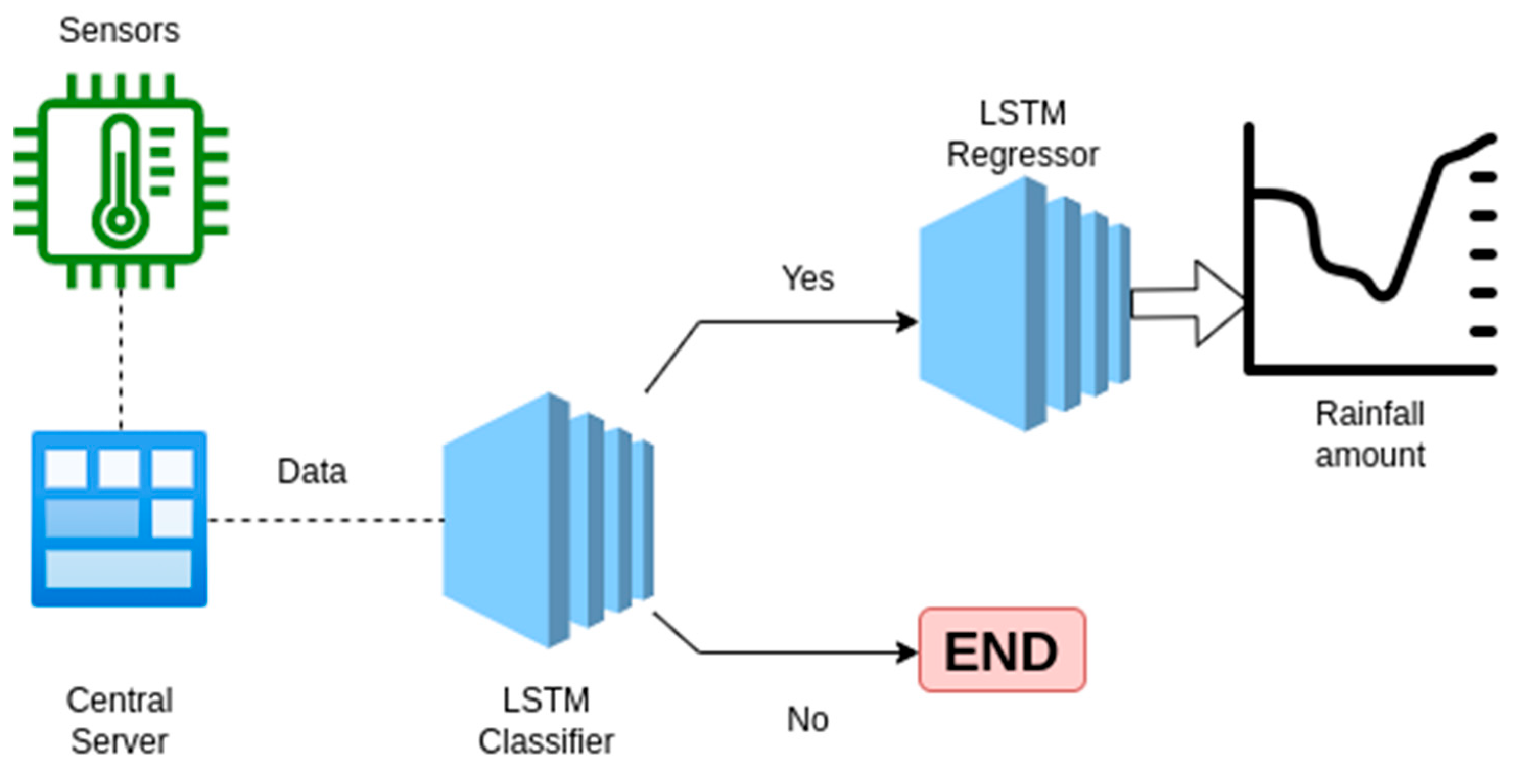
The developed machine learning pipeline, which is shown in Figure 2, consists of the following steps:

• Data collection and transformation. Data are collected from the meteorological station with a 10 min frequency and transformed, as already explained, in order to become consumable by the machine learning models.
• Classification. The data are consumed using a classification model, namely, the deep LSTM classifier, which dictates whether a rainfall event will occur in the next time step. In case of a rainfall event, the classifier outputs one, or otherwise zero.
• Regression. If a rainfall event is predicted, the execution of a second machine learning model is triggered. The model, i.e., the deep LSTM regressor, assesses the amount of the anticipated rainfall, using the same input as the deep LSTM classifier.

The forecasting horizon is 10 min for both models. The development and the training of the models was carried out using PyTorch [10], a Python wrapper of a machine learning library that enables high-performance computations.

2.2.1. Deep LSTM Classifier

Regarding the architecture of the classifier, there is an LSTM in the first layer. At the top of it, several dense layers are stacked. These are followed by the output layer, i.e., a sigmoid function.

The sigmoid function is chosen because there are two classes. The first class corresponds to an occurrence of a rainfall event and the output of the sigmoid function, after rounding it, is one. The second class corresponds to non-events and the output of the sigmoid function, after rounding it, is zero.

The number of dense layers in the network and the nodes number in each layer of the network are defined during the training phase using Ray Tune [11], a hyperparameter grid search tuner.

The loss function used in the training phase is the binary cross-entropy loss. The model is trained using 10 features, corresponding to the columns of the dataset, as listed in Section 2.1.

2.2.2. Deep LSTM Regressor

The architecture of the deep LSTM regressor includes an LSTM as the first layer, followed by several dense layers and the output layer, which has a single node that applies a linear transformation in its input. The deep LSTM regressor outputs the amount of rain for the upcoming event and is triggered by the anticipation of a rainfall event.

The number of dense layers in the network and the number of nodes in each layer of the network are defined during the training process in a similar fashion to the deep LSTM classifier.

Because the deep LSTM regressor is used only in the case of an upcoming (predicted) rainfall event, it is trained using data that contain only such events. To do so, a new time series is built including values within a predefined time window that includes the rainfall event and certain time steps before and after.

The loss function used for the training phase is the mean-square-error. The inputs of the deep LSTM regressor are those used for the deep LSTM classifier, plus the current rainfall amount.

2.2.3. Tuning of the Hyperparameters

The hyperparameters are tuned using a grid search approach. The implementation is based on the Ray Tune scheduler [11]. The hyperparameters to be tuned and the search field of their optimal values are shown in

Table 1. The hyperparameters to be tuned and their search space.

Nr.	Hyperparameter	Search Space
1	Lookback time window	1 to 24 time steps 1
2	Number of dense layers	1 to10 layers
3	Number of neurons	2 ^ i, where i = 0, 1, …, 10
4	Learning rate of the training algorithm	9 × 10−6, 9 × 10−1

¹ Each time step corresponds to 10 min.

. For each combination of these hyperparameters, a new neural network is built, trained and tested.

3. Results

The best architecture for the deep LSTM classifier includes six hidden layers with 1000 nodes each, trained with a learning rate of 6 × 10⁻⁶ and a time window of 24 (4 h). The model achieved accuracy = 96.45%, precision = 97.78%, recall = 94.82% and AUC = 96.41%.

The best architecture for the deep LSTM regressor comprises one hidden layer with 100 nodes and is trained with a learning rate of 9 × 10⁻⁵ and a time window of 24 (4 h). The model achieved an MSE = 6.635, MAE = 1.417 and MAPE = 1.235. In Figure 3, the actual amount of rainfall is compared with the predicted amount.

4. Discussion

The results show that the deep LSTM models are capable of predicting both the occurrence of rain events and the amount of rain with increased levels of accuracy. Also, since the weather station rainfall sensor has a resolution of 0.2 mm and given that the predictions can be rounded to the nearest value, the forecast errors are even smaller, matching the 0.2 mm intervals. The predictive capability, and the fact that only in situ measurements were taken into account as inputs in the machine learning pipeline, make the proposed solution consistent with the requirements of real-world applications.

The future work of the present study is based on three pillars. The first includes tests of different machine learning technologies. In particular, the predictive capability of machine learning models featuring the attention mechanism and models based on transformers will be assessed. The second pillar includes tests regarding the forecasting horizon and its extension. The third pillar concerns transfer learning, meaning the reuse of the presented models (i.e., trained using data registered to the island of Nisyros) to predict rainfall events and the amount of rainfall in a nearby island, namely Tilos, where data are continuously collected from a weather station and where the climate has similar characteristics to Nisyros.

5. Conclusions

In the present study, a machine learning pipeline was developed using solely in situ data registered to a meteorological station located on the island of Nisyros in the South Aegean Sea in Greece. The dataset contains rainfall, mean, lowest and highest temperature measurements as well as measurements of the relative humidity, the atmospheric pressure, the wind speed, the highest wind speed in the horizontal plane, and the wind direction. These features are used to train two machine learning models. The first model, namely the deep LSTM classifier, performs classification, predicting whether it is going to rain in the near future (10 min forecasting horizon). The second model, namely the deep LSTM regressor, predicts the amount of rainfall, having the same forecasting horizon and inputs as the former network. Each model is trained using time series data that contain exclusively rain events. The length of the time series as well as the number of the networks’ layers are treated as hyperparameters and determined during the training phase using a grid search approach. The results show that the developed models are suitable for short-term rainfall forecasts, having MAEs of 1.4 mm. Also, the proposed machine learning pipeline triggers the execution of the deep LSTM regressor only when the classifier predicts the occurrence of a rainfall event, reducing the computational requirements while allowing for the use of a dataset that contains exclusively rainfall events in the regressor’s training process, which, in turn, results in increasing forecasting performance.

References

- Basha, C.Z.; Bhavana, N.; Bhavya, P.; Sowmya, V. Rainfall prediction using machine learning & deep learning techniques. In Proceedings of the 2020 International Conference on Electronics and Sustainable Communication Systems (ICESC), Coimbatore, India, 2–4 July 2020; IEEE: Toulouse, France, 2020; pp. 92–97. [Google Scholar]
- Moustris, K.P.; Larissi, I.K.; Nastos, P.T.; Paliatsos, A.G. Precipitation forecast using artificial neural networks in specific regions of Greece. Water Resour. Manag. 2011, 25, 1979–1993. [Google Scholar] [CrossRef]
- Pham, B.T.; Le, L.M.; Le, T.-T.; Bui, K.-T.T.; Le, V.M.; Ly, H.-B.; Prakash, I. Development of advanced artificial intelligence models for daily rainfall prediction. Atmos. Res. 2020, 237, 104845. [Google Scholar] [CrossRef]
- Shrivastava, G.; Karmakar, S.; Kowar, M.K.; Guhathakurta, P. Application of artificial neural networks in weather forecasting: A comprehensive literature review. Int. J. Comput. Appl. 2012, 51, 17–29. [Google Scholar] [CrossRef]
- Salehin, I.; Talha, I.M.; Hasan, M.M.; Dip, S.T.; Saifuzzaman, M.; Moon, N.N. An Artificial intelligence-based rainfall prediction using LSTM and neural network. In Proceedings of the 2020 IEEE International Women in Engineering (WIE) Conference on Electrical and Computer Engineering (WIECON-ECE), Bhubaneswar, India, 26–27 December 2020; IEEE: Toulouse, France, 2020; pp. 5–8. [Google Scholar]
- Qing, X.; Niu, Y. Hourly day-ahead solar irradiance prediction using weather forecasts by LSTM. Energy 2018, 148, 461–468. [Google Scholar] [CrossRef]
- Karevan, Z.; Suykens, J.A. Transductive LSTM for time-series prediction: An application to weather forecasting. Neural Netw. 2020, 125, 1–9. [Google Scholar] [CrossRef] [PubMed]
- Salman, A.G.; Heryadi, Y.; Abdurahman, E.; Suparta, W. Single layer & multi-layer long short-term memory (LSTM) model with intermediate variables for weather forecasting. Procedia Comput. Sci. 2018, 135, 89–98. [Google Scholar]
- Lagouvardos, K.; Kotroni, V.; Bezes, A.; Koletsis, I.; Kopania, T.; Lykoudis, S.; Mazarakis, N.; Papagiannaki, K.; Vougioukas, S. The automatic weather stations NOANN network of the National Observatory of Athens: Operation and database. Geosci. Data J. 2017, 4, 4–16. [Google Scholar] [CrossRef]
- PyTorch. Available online: https://pytorch.org/ (accessed on 28 June 2023).
- RayTune. Available online: https://docs.ray.io/en/latest/tune/index.html (accessed on 28 June 2023).