Stationary/Non-Stationary Modelling for Extreme Value Distribution: Analysis of Rainfall Annual Maxima in Italy in a Climate Change Context ^†

Abstract

In this paper, EXTRASTAR software (EXTRemes Abacus for STAtistical Regionalization) is illustrated, which provides a general framework for extreme value analysis, specifically for Annual Maxima (AM) time series. The proposed methodology represents a useful and quick approach to carry out onsite and regional statistical investigations of extreme events, which is also suitable for climate change scenarios. EXTRASTAR was tested with the AM time series at daily resolutions for the entire Italian rain gauge network by implementing EV1 (Extreme Value Type I), GEV (Generalized Extreme Value) and TCEV (Two-Components Extreme Value) probability distributions.

1. Introduction

From the literature, statistical analysis of hydrological extremes can be diversified according to: (1) the adopted probability function; (2) the type of approach: stationary (i.e., temporal invariance of model parameters) or non-stationary (i.e., model parameters are time-varying to account for climate change scenarios); (3) the method for parametric estimation (onsite or regional), based on the sample size; (4) the specific technique for parametric estimation (method of moments, maximum likelihood, least squares, and so on). Therefore, a technician has many combinations for statistical analysis of extreme values, even in possible climate change scenarios.

In this framework, the paper describes a quick methodology implemented within the EXTRASTAR software (EXTRemes Abacus for STAtistical Regionalization), a user-friendly Excel file with macros in VBA (Visual Basic for Application).

EXTRASTAR was tested for the Italian network of annual maxima (AM) of daily rainfall time series, related to the SCIA database of the Italian Institute for Environmental Protection and Research-ISPRA (www.scia.isprambiente.it, accessed on 31 January 2022).

The obtained results have shown that EXTRASTAR can be considered a useful tool for obtaining quick indications about possible clusters of different time series in statistically homogeneous areas, as well as a reduction in the computational cost for onsite parametric estimates.

2. Methods and Material

2.1. Theoretical Background on Adopted Probability Functions

Firstly, assuming a stationary context, the following probability models were implemented in EXSTRAR for the statistical analysis of the AM series in terms of Cumulative Density Functions (CDF):

EV1 [1]

$$F_X\left(x\right)=P\left[X\le x\right]=e^{-e^{-\left(\frac{x}{\theta }-ln\mathsf{\Lambda }\right)}}$$

(1)

where $\mathsf{\Lambda }$ represents the mean annual number of occurrences with a magnitude greater than a prefixed threshold (under the hypothesis of a homogeneous Poisson process for the occurrences), while $\theta$ corresponds to the annual mean value for the associated intensities (by assuming an exponential distribution for this process).

GEV [2]

$$F_X\left(x\right)=P\left[X\le x\right]=e^{-{\left[1-b\left(\frac{x}{\theta }-ln\mathsf{\Lambda }\right)\right]}^{1/b}}$$

(2)

where, in addition to $\mathsf{\Lambda }$ and $\theta$, there is the shape parameter $b$. In this case, preserving the hypothesis of a homogeneous Poisson process for the occurrences, it is assumed that the process of intensities above a threshold follows the Generalized Pareto distribution. It is well-known that GEV coincides with the EV1 for $b$ = 0, while EV2 and EV3 distributions are obtained when $b$ < 0 and $b$ > 0, respectively.

TCEV [3]

$$F_X\left(x\right)=P\left[X\le x\right]=e^{-{\mathsf{\Lambda }}_1{e}^{-\frac{x}{{\theta }_1}}-{\mathsf{\Lambda }}_2{e}^{-\frac{x}{{\theta }_2}}}$$

(3)

in which ${\mathsf{\Lambda }}_1$ and ${\mathsf{\Lambda }}_2$ (with ${\mathsf{\Lambda }}_1>{\mathsf{\Lambda }}_2$) are the mean annual number for ordinary and outlier events, respectively, while ${\theta }_1$ and ${\theta }_2$ (with ${\theta }_1<{\theta }_2$) are the correspondent mean values for intensities. A well-known TCEV formulation, used in contexts of statistical regionalization, is obtained by introducing two dimensionless parameters ${\theta }_{*}={\theta }_2/{\theta }_1$ and ${\mathsf{\Lambda }}_{*}={\mathsf{\Lambda }}_2/{\mathsf{\Lambda }}_1^{1/{\theta }_{*}}$:

$$F_X\left(x\right)=e^{-{\mathsf{\Lambda }}_1{e}^{-\frac{x}{{\theta }_1}}-{\mathsf{\Lambda }}_{*}{\mathsf{\Lambda }}_1^{1/{\theta }_{*}}{e}^{-\frac{x}{{\theta }_{*}{\theta }_1}}}$$

(4)

Obviously, an ad hoc procedure for statistical regionalization can be developed for any probability distribution [4]. For the implemented models in EXTRASTAR, the reduced EV1 variable [3] is considered:

$$Y=\frac{X-\theta ln\mathsf{\Lambda }}{\theta }=\frac{X-{\theta }_{1}ln{\mathsf{\Lambda }}_1}{{\theta }_1}$$

(5)

As Y is a linear transformation of X, these two random variables clearly present the same value for skewness.

Then, it is possible to rewrite Equations (1)–(4) as:

$$\mathrm{EV}1:F_Y\left(y\right)=e^{-e^{-y}}$$

(6)

$$\mathrm{GEV}:F_Y\left(y\right)=e^{-{\left(1-by\right)}^{1/b}}$$

(7)

$$\mathrm{TCEV}:F_Y\left(y\right)=e^{-e^{-y}-{\mathsf{\Lambda }}_{*}{e}^{-y/{\mathsf{\theta }}_{*}}}$$

(8)

and to identify Homogeneous Regions (HRs), where the theoretical skewness, and therefore the parameters ${\mathsf{\Lambda }}_{*}$ and ${\theta }_{*}$ for the TCEV, or the parameter $b$ (with $b$ = 0 in the case of EV1) for the GEV, can be assumed as constant [5] or they follow laws based on geomorphological covariates (altitude, hydrographic basin area, etc.).

The developed methodology in EXTRASTAR (useful for either onsite or regional approaches) is based on the following steps:

• Sample sizes N between 20 and 200 were considered. For each N and for each distribution, 5000 series of the variable Y were generated using the Monte Carlo methodology [6]. In detail: (i) for GEV, the following six values of parameter b were considered: 0 (EV1), −0.05, −0.1, −0.15, −0.2, −0.25; (ii) 32 combinations of (${\mathsf{\Lambda }}_{*}$, ${\theta }_{*}$) were used for TCEV, with $0.1\le {\mathsf{\Lambda }}_{*}\le 0.5$ (step 0.1) and $1.5\le {\mathsf{\theta }}_{*}\le 5$ (step 0.5). Overall, 38 × 5000 samples of the standardized variable Y were generated for each value of N;
• for each set of 5000 series, the 90% confidence band was evaluated for the sample skewness g; therefore, 38 confidence bands for each N can be represented within an abacus, implemented within the EXTRASTAR software.

By inserting, into the abacus, the information from AM time series, in terms of N and g, it is possible to quickly assess which distributions (and with reference values of the shape parameters) can model the sample skewness (and then the possible presence of outliers), and therefore to cluster some/many series in HRs.

It should be highlighted that this methodology can also be useful in climate change contexts, mainly for specific time resolutions (e.g., daily) for which the hypothesis of stationarity could not be rejected in many cases. A detailed, state-of-the-art trend analysis for the Italian AM rainfall series is reported in [7].

Moreover, it should be stated that the concept of “change” is not mutually exclusive with the term “stationarity” [8]. In fact, according to the examples with Newton’s laws: (1) without an external force, the position of a body in motion changes in time, but the velocity is unchanged; (2) a constant force implies a constant acceleration and a changing velocity. Consequently, change is a general notion applicable to the real world, while stationarity and non-stationarity only regard the adopted models to explain the observed data. In some/many cases, changes are more evident for specific spatial and temporal resolutions, with respect to others (for which a stationary approach can be sufficient to model the sample series).

In this context, results from simple numerical experiments are below illustrated. Specifically, starting from an EV1 distribution in terms of the Y variable (Equation (6)):

• A total of 5000 sets of 100 Y data were generated with the Monte Carlo methodology;
• From Equation (5), the authors calculated the correspondent values for the X variable as:

  $$X\left(t\right)=\theta \left(t\right)·\left(Y+ln\mathsf{\Lambda }\right)={\theta }_0·\left(1+\alpha ·t\right)·\left(Y+ln\mathsf{\Lambda }\right)$$

  (9)

  i.e., by considering $\mathsf{\Lambda }$ as invariant, while an increasing linear trend for $\theta$ is assumed, where ${\theta }_0$ and $\alpha$ are prefixed initial value and trend rate, respectively, and $1\le t\le N$;
• For a considered trend rate $\alpha$, and varying the sample size N from 20 to 100, the Mann–Kendall test [9,10] was applied for each synthetic sample of X, for which it is easy to demonstrate that the statistic Z_MK does not depend on the initial value ${\theta }_0$, because of these specific assumptions of EV1 population and invariance for $\mathsf{\Lambda }$;
• The percentages of synthetic samples with |Z_MK| > 1.96 (i.e., the null hypothesis of no trend is rejected at 5% significance level) are represented in Figure 1 for three values of trend rate $\alpha$ (10%, 20% and 50% in 100 years) and different invariant values for $\mathsf{\Lambda }$.

The obtained results highlight that there is a significant percentage of synthetic samples for which the assumed change for $\theta$ does not imply |Z_MK| > 1.96, and then a stationary modelling could be adopted for statistical analysis in these cases.

2.2. Data Set

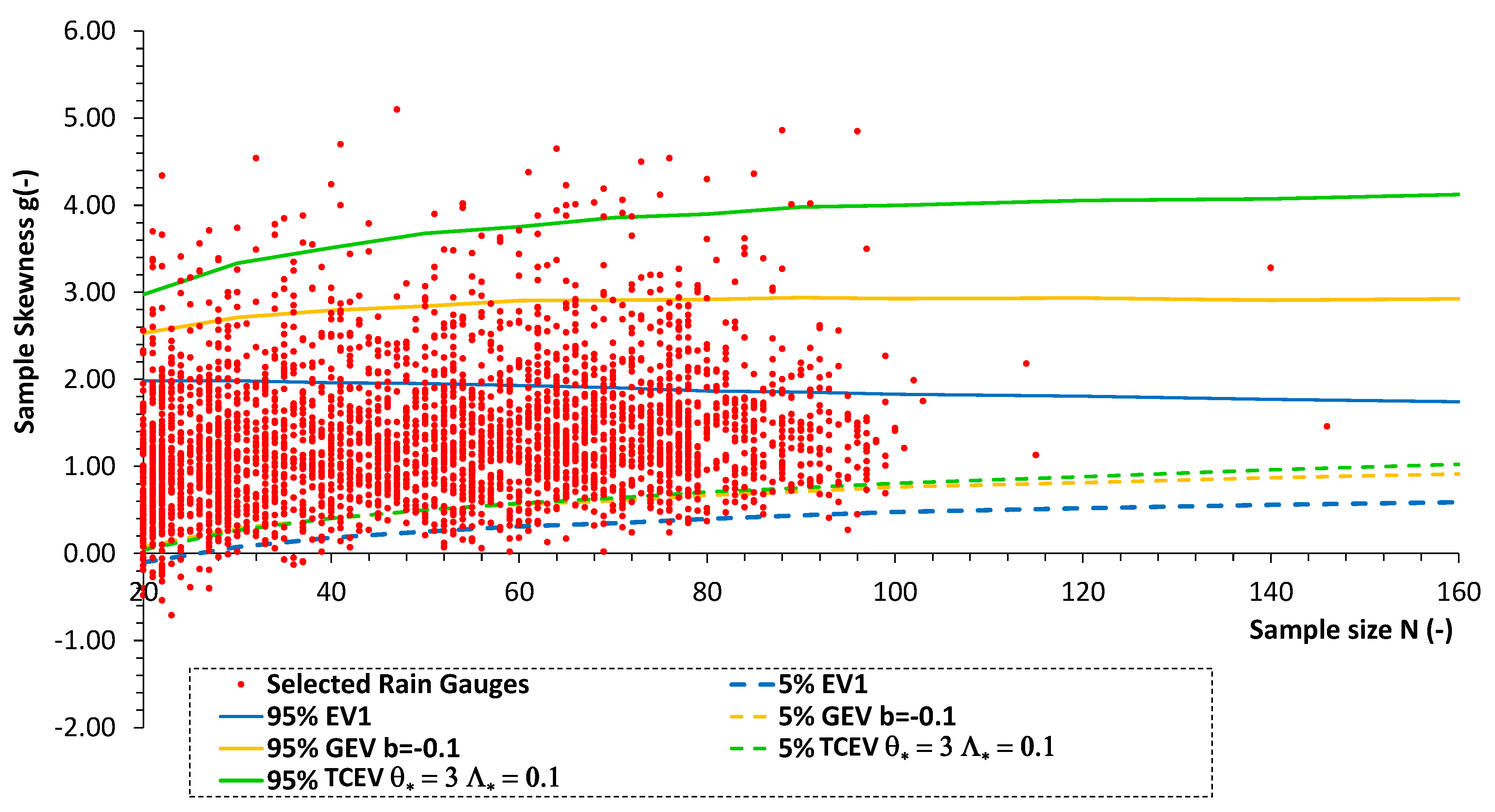
The main input for EXTRASTAR is a two-column .txt file (without headers), in which the ith row contains sample size N (first column) and sample skewness g (second column) of the ith AM series. In this work, the used input file was obtained from the SCIA database of the Italian Institute for Environmental Protection and Research-ISPRA (www.scia.isprambiente.it, accessed on 31 January 2022) regarding the network of daily AM rainfall series. Overall, 3351 samples with N > 20 years in the time interval 1860–2020 were analyzed. The mean value of N is approximately 50 years, with a maximum of 146 years (Milan rain gauge). The values of g varied from −0.71 to 5.10, with an average of 1.34. The software allows for the display of the pairs (N, g) on the abacus, together with the 90% confidence bands relating to EV1 law (inserted by default) and to GEV and TCEV distributions with values of parameters b (GEV) and ${\mathsf{\Lambda }}_{*}$, ${\theta }_{*}$ (TCEV), which are selected by the user through a dedicated form. The abacus is structured in such a way as to represent only one option at a time for both GEV and TCEV to simplify the visualization of the results (Figure 2).

3. Results and Discussion

From the analysis of the abacus, it is possible to assess that: (1) the EV1 model allows for the reconstruction of sample skewness for almost 80% of cases (i.e., 2679 samples); (2) the use of the shape parameter b = −0.1 (among all the considered values) provides the best modeling with the GEV law: 88.7% of cases, equal to 2971 sample series. Moreover, 2526 series from this subset (i.e., the 75.4% of the whole data set) can be modeled with EV1; (3) the sample skewness of 3064 time series (91.4% of the entire data set) can be reconstructed through the TCEV law with ${\mathsf{\Lambda }}_{*}$= 0.1 and ${\theta }_{*}$= 3. From this subset, the 2520 series (75.2 % of the whole data set) can be modelled with the EV1 and 2961 series (88.4% of the entire data set) with GEV distribution with b = −0.1.

As an example of an application for a single daily AM time series, the authors focused on the Subiaco rain gauge (close to Rome), characterized by N = 103, g = 1.53, and an average of 68.8 mm with a standard deviation of 21.1 mm. The Mann–Kendall test provided a value of the statistic Z_MK equal to 1.39 over the entire time series and to 1.91 if we consider the data from 2000. In both cases, the absolute value of Z_MK is less than 1.96, then it is possible to not reject the hypothesis of a stationary process with a significance level of 5%. By inserting the information (N = 103, g = 1.53) on the EXSTRASTAR abacus, it emerges that Subiaco AM series can be modeled with EV1 and with GEV−b = −0.1 and TCEV−${\mathsf{\Lambda }}_{*}$ = 0.1 and ${\theta }_{*}$ = 3.

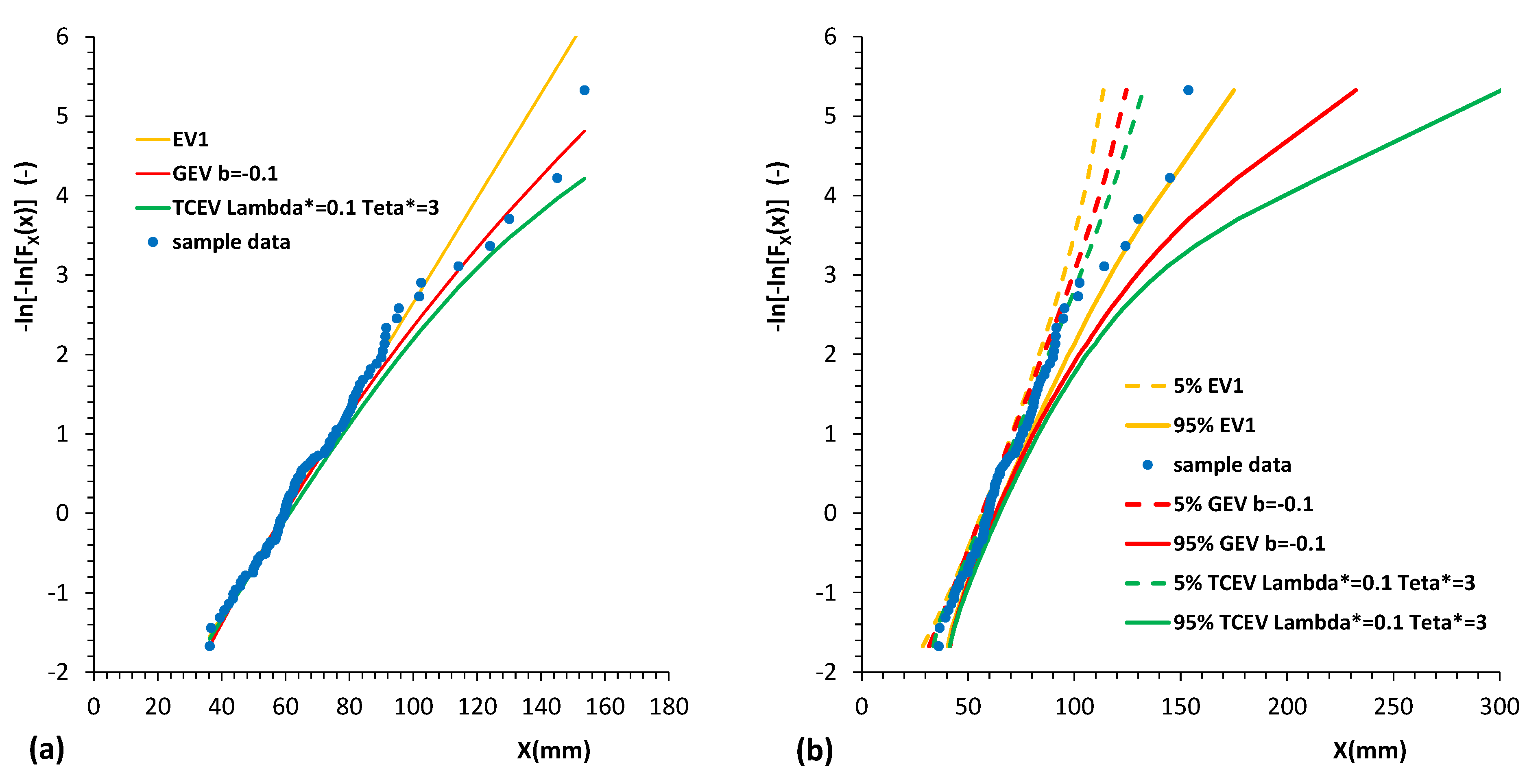
The Maximum Likelihood (ML) estimates for EV1 distribution provided θ = 15.2 mm and Λ = 50.7. The ML technique usually allows for an excellent fitting of the data with respect to ordinary values. Assuming these estimates also for the corresponding parameters of GEV and the ordinary component of TCEV, authors obtained the comparison on the EV1 probabilistic plot (Figure 3a), from which the EV1 and TCEV laws could be considered inadequate. On the contrary, if 5000 synthetic Monte Carlo generations (each one with N = 103) are carried out for each considered probabilistic laws, and the corresponding 90% confidence bands are estimated, it is clear that each distribution may not be rejected for the modeling of the investigated sample series (Figure 3b), thus confirming what is hypothesized with the abacus analysis. Obviously, in the context of parsimony, a two-parameter distribution would be preferred.

4. Conclusions

The EXTRASTAR software can undoubtedly represent a user-friendly tool for the statistical analysis of annual maxima, even in the context of a climate change scenario. For an observed time series of interest, it is possible to quickly test the modelling capability for EV1 and GEV or TCEV, also with reference values for the shape parameters (b for GEV, and ${\mathsf{\Lambda }}_{*}$and ${\theta }_{*}$ for TCEV), on the basis on the sample size and skewness.

Furthermore, by simultaneously analyzing the sample skewness of several time series, a user can obtain a quick indication of potential clusters in homogeneous regions.

Furthermore, the use of EV1 Maximum Likelihood estimates also for GEV and the ordinary component of TCEV allows for a reduction of the computational costs with respect to carry out a specific calibration procedure for each probability function.

Future developments will concern the implementation, within EXTRASTAR, of specific modules for modeling with non-stationary approaches to account for any effects of climate change.

References

1. Gumbel, E.J. Statistics of Extremes; Columbia University Press: New York, NY, USA, 1958. [Google Scholar]
2. Jenkinson, A.F. The frequency distribution of the annual maximum (or minimum) values of meteorological elements. Q. J. R. Meteorol. Soc. 1955, 81, 158–171. [Google Scholar] [CrossRef]
3. Rossi, F.; Fiorentino, M.; Versace, P. Two-component extreme value distribution for flood frequency analysis. Water Resour. Res. 1984, 20, 847–856. [Google Scholar] [CrossRef]
4. Ferrari, E.; Versace, P. La Valutazione delle Piene in Italia. Rapporto di Sintesi GNDCI. 1994. Available online: http://www.idrologia.polito.it/gndci/rapportiPdf/Vapi_Nazionale.pdf (accessed on 31 January 2022). (In Italian).
5. Gabriele, S.; Arnell, N. A hierarchical approach to regional flood frequency analysis. Water Resour. Res. 1991, 27, 1281–1289. [Google Scholar] [CrossRef]
6. Kottegoda, N.T.; Rosso, R. Applied Statistics for Civil and Environmental Engineers; Blackwell: Oxford, UK, 2008. [Google Scholar]
7. Caporali, E.; Lompi, M.; Pacetti, T.; Chiarello, V.; Fatichi, S. A review of studies on observed precipitation trends in Italy. Int. J. Climatol. 2021, 41, E1–E25. [Google Scholar] [CrossRef]
8. Koutsoyiannis, D.; Montanari, A. Negligent killing of scientific concepts: The stationarity case. Hydrol. Sci. J. 2014, 60, 1174–1183. [Google Scholar] [CrossRef]
9. Mann, H.B. Non-parametric tests against trend. Econometrica 1945, 13, 245–259. [Google Scholar] [CrossRef]
10. Kendall, M.G. Rank Correlation Measures; Charles Griffin: London, UK, 1975. [Google Scholar]
Figure 1. Percentages of synthetic samples (from a transient EV1 distribution) with |ZMK| > 1.96 for a different trend rate related to θ : (a) +10% in 100 years; (b) +20% in 100 years; (c) +50% in 100 years.
Environsciproc 21 00065 g001
Figure 2. Plot of EXTRASAR abacus, with information from SCIA database of ISPRA (www.scia.isprambiente.it, 31 January 2022) concerning the Italian network of daily AM rainfall series.
Environsciproc 21 00065 g002
Figure 3. Daily AM series of Subiaco rain gauge: (a) comparison with EV1, GEV (b = −0.1) and TCEV ( Λ * = 0.1 e θ * = 3 ) distributions; (b) comparison with 90% confidence bands for the investigated distributions.
Environsciproc 21 00065 g003
Publisher’s Note: MDPI stays neutral with regard to jurisdictional claims in published maps and institutional affiliations.