Abstract
Nature-Based Solutions (NBSs) are considered worldwide as a suitable approach for mitigating the impact of industrial agriculture on sediments and nutrient losses. However, their actual effectiveness is still questioned. In cases where site measurements of NBS performance are scarce, models can provide useful insights if accurately set. This study analyzed the effects of vegetated buffer strips (VBSs) and winter cover crops (WCCs) planted in some herbaceous cropping systems within the Massaciuccoli reclamation area (Vecchiano, Central Italy). Analyses stem from modelling water and soil dynamics by applying SWAT+ at field scale on high resolution close-range photogrammetric digital terrain model (DTM), real crop rotations, and a detailed calendar of the main agronomic interventions. The NBS implementation was modelled in two experimental areas, showing contrasting soil properties. Comparing results from the modelling of different scenarios highlighted that NBS mitigative effect is influenced by soil properties and local topographic irregularities, which could induce concentrated flows. Long term climate changes can induce relevant different effects by varying the nature of soil.
1. Introduction
Runoff and sediment losses in temperate areas are triggered mainly by rainfalls [1,2]; many other predisposing factors affecting runoff and soil erosion are also known. The most relevant are soil properties, organic content, land cover and use, slope angle, slope length, and agricultural and conservation practices [3,4]. In agricultural areas, where annual crops are the most widespread practices, the relationship between the stage of plant growth and rainfall events strongly affects the rainfall/runoff ratios [5] and consequently the soil erosion. Hazard modelling should thus consider a time interval covering the entire plant lifecycle to properly account for the different plant growth stages when different rainfall events occur. On the other hand, to include the effects of short-term rainfalls, time sampling should be accurate enough to reproduce each single event. Such time scales (from one to many years) are not suitable for identifying return periods due to the uncertainty of medium to long-term climatic cyclicality. Therefore, the assessment of runoff and soil erosion, and the potential changes due to the implementation of mitigative countermeasures, could be more oriented to areal susceptibility than to hazards in the strict sense, and climatic variations should be accounted for over long periods of time.
In such a framework, the effects of mitigative actions could be properly estimated by comparing baseline and post operam scenarios during modelling.
To assess the residual susceptibility over long-term accounting for climate changes, such a comparison could be carried out considering modelled weather data for different climatic scenarios (i.e., IPCC RCP 4.5 and RCP 8.5 [6,7]), considering the furthest period available (years up to 2100).
When runoff and soil erosion are modelled on flat agricultural areas, the model should be carefully chosen among those able to both deal with almost flat morphologies and implement agricultural practices.
With the approach used here to model runoff and soil erosion in two farms in the Massaciuccoli catchment (Central Italy), the modelling capability to deal with local scales (plot to farm-scale) was considered when choosing the proper method and modelling software. Moreover, the modelling approach was also based on the model suitability to implement the type of countermeasures implemented in the study area, namely nature-based solutions (NBS) such as vegetated buffer strips (VBS) and winter cover crops (WCC), and to model the hazard they are dealing with, namely runoff and soil loss.
Many models are available in the literature focusing on runoff and soil erosion working at different scales and with different approaches ranging from fully empirical models to physically-based models for soil erosion and water runoff up to physically-based models directly simulating pollutant runoff. In Table 1, the main strengths and limitations, referring to the abovementioned requirements, are synthesized for four soils, and water assessment models applied worldwide. All four models allow for the consideration of the implementation of NBSs such as VBS and WCC. Among these, the Soil and Water Assessment Tool (SWAT) [8], and the revised version SWAT+ [9] are extensively supported by scientific literature documenting their applications at different scales and morphologies [10,11,12,13]. These models were frequently employed to simulate the effect of VBS and WCC [14,15]. Moreover, they provide spatialized results as georeferenced shapefiles, ranging from sediment budgets and water balances and nutrient losses referred to both landscape units and hydrographic networks [16]. Simulations are based on large periods (up to many years) but with a daily temporal resolution [8], allowing for estimates for weather events of a medium duration (a few days). On the other hand, they are quite high data-demanding and need huge computational capacity, especially when modelling high-resolution data.

Table 1.
Comparison of different runoff and soil erosion models. For each model, the acronym of the satisfied requirement is reported. Ma = requirement in terms of the type of matrices considered in modelling (e.g., runoff, soil loss, nutrient loss etc.); S = requirements for the scale of the assessment; Mo = requirements in terms of morphologies allowed for modelling (e.g., slopes, flat areas etc.); D = requirements in terms of dimensionality of the model (1D–2D–3D) and capability to spatialize results.
Study Area
The present work aims at testing some NBSs such as VBS and WCC in flat agricultural areas, and estimating the impacts of different soils on their mitigative effect. For this purpose, two farms (namely the Studiati and Gioia) to the south of the Massaciuccoli Lake are considered. Here, an important marshy area reclaimed in the 1920s was turned into agricultural land. Soils are characterized by fluvial to lacustrine surficial deposits ranging from silty clays to the south, which gradually change to sands moving to the north. The organic content (OC) remarkably increases when approaching the lake, ranging from <3% in the southern part to up to 55% close to the southernmost lake embankments.
The two test sites are representative of such contrasting pedological features with the Gioia area, to the south, characterized by fine-grained mineral soils (OC < 4%) and the Studiati’s, to the east, showing coarse-grained peat soils (OC > 20%). In both areas, in the frame of the H2020 PHUSICOS project [20], VBSs and WCCs were implemented in some plots, mainly aimed at reducing sediment transport and runoff.
The efficacy of such NBSs is modelled under different pedological and climatic conditions. To this aim, different scenarios were set up in SWAT+ environment for result comparison. They consisted of: (1) a control (baseline) scenario (S0), implementing conventional agricultural practices, (2) an NBS scenario, implementing both 3 m-wide VBS and WCC. Both scenarios were modelled under different climatic settings such as current climate (referring to the 2010–2015 period); future long-term mild climate changes (RCP 4.5 scenario simulated for the period 2095–2100); future long-term strong changes (RCP 8.5 scenario simulated for the period 2095–2100). Since the main purpose is to estimate runoff and soil losses at local (farm) scales, high resolution input data were set in the model.
2. Methods
Type of input data and their accuracy for running the SWAT model mostly depend on the scale of the assessment. They concern: (1) soil properties which can be derived from available regional databases or from local sample data; (2) DTM at suitable resolution for representing the scale of the hydrographic network; (3) land use maps at the proper scale; (4) weather data. For large scale applications, high-resolution data assure the reliability of the modelling results.
The DTM used for simulations was derived from close-range 20 cm cell size photogrammetry with dm-scale roughness affecting surficial water flow. Therefore, DTM post-processing procedures were essential to delineate watersheds and hydrographic networks consistently with those detected in the field. To this aim, both the automatic “burn-in” function of SWAT+ [21] and manual DTM carving were applied, resulting in a hydraulically consistent watershed and draining network delineation.
Soil maps were interpolated on local soil data derived from Silvestri et al. [22] (Figure 1). Most of the required parameters were directly measured by the authors (sand, silt and clay percentages; USDA classification; organic matter per cent content; PH; electrical conductivity; albedo ratio; CaCO3 per cent content). The remaining parameters were obtained by applying empirical pedo-transfers developed on similar soil types. Specifically, bulk density (BD) available water content (AWC), USLE soil erodibility (kUSLE) were set through empirical equations [23,24,25]. The hydraulic conductivity (Ksat) was derived from direct measurements on soils with similar textures and organic content in comparable contexts, instead.
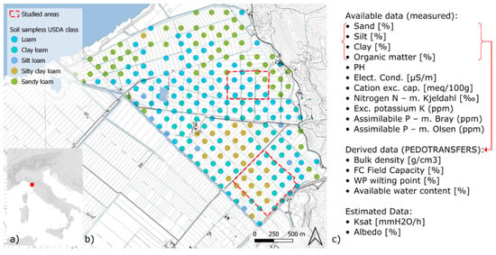
Figure 1.
(a) Inset of the study area; (b) soil sample [22] used for raster interpolation and zonal statistics, classified based on USDA textures; (c) list of input parameters demanded for modelling distinguishing the measured data, data derived by empirical equations, based on input parameters included in red curly brackets, and data estimated based on similar soil samples in the same setting.
SWAT+ soil input data were set discretizing the continuous variables in individual soil units based on soil textures and organic content. Soil units were then used for zonal statistics to estimate the mean values of the remaining parameters.
Input maps of land use were used to differentiate S0 from NBS scenarios (S1), by specifying the cycles of crop rotation and the type of land cover on areas interested by the NBSs. The land use maps were delineated based on remote sensing on the high-resolution orthophoto and DTM and implementing the NBS design layouts. High-resolution data allowed for the mapping of individual plots with different crop-rotation; given the large scale of the analysis, VBSs and areas interested by WCCs were also mapped as individual polygons, thus representing the real extension of the measures’ implementation (Figure 2c,f). The different land-use units mapped were linked to new codes implemented in the SWAT + SQL database and characterized by different crop rotations schemes, for which calendars of agrotechnical operation were collected from farmers. A complete set of information about the agricultural operations was available for both areas since 2010; therefore, modelling was carried out in the time interval 2010–2015. Actual operations were represented in the model by implementing proper management operation schedules over the whole period, for each crop rotation scheme (land-use type) carried out different land parcels (Figure 2a,d). In such a way, the actual calendars were used rather than automatic scheduling. For hydrological response units (HRUs) interested by NBSs, two different schedules were developed representing S0 and S1, respectively, thus scheduling only conventional agrotechnical operations or implementing VBSs and WCC operation cycles.
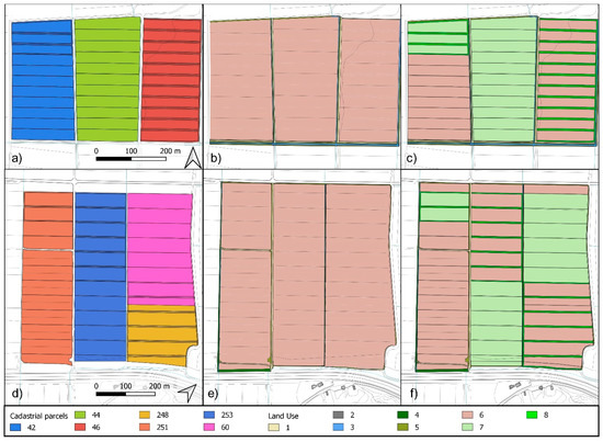
Figure 2.
Land-use map used as input in SWAT+. They are differentiated based on cadastral parcels interested by different crop rotations schemes in the Studiati (a) and Gioia (d) areas, land use for the baseline scenario S0 (b,e), land use for the scenario S1 accounting for different agricultural techniques (c,f). Cadastral parcels: identified according to official ID: 42, 44, 46, 248, 251, 253, 250; Land use: 1 = unpaved rural roads, 2 = paved roads/areas, 3 = water bodies, 4 = uncultivated bushy areas, 5 = uncultivated grassed areas, 6 = conventional agriculture, 7 = conservative agriculture (S1), 8 = vegetated buffer strips (S2).
Given the local scale of the modelling, the high-resolution of input data, and the availability of local data from a weather station close to the study area (the Metato station sited 4.8 km to the south [26]), the use of observed weather data was preferred. A complete set of data on rainfall, temperature, humidity, wind velocity and direction, and solar radiation was available with a 15 min time interval since 2010, with very few gaps. Only temperature and rainfall depth were available for previous periods (since 1990). Based on local data used for model downscaling and calibration [27,28,29,30], future data for the RCP 4.5 and 8.5 climatic scenarios were modelled with Climate Change Toolkit (CCT) [31].
3. Results and Discussion
The approach used provided detailed estimates of agricultural practices and NBSs performances regarding site runoff and soil erosion dynamics with their spatial distribution referred to spatial units defined as HRUs [9,12,32] with a resolution of a few square meters.
The study focused on the annual average runoff depths and sediment yield rates, the latter consisting of the areal average of the sediment detached from each HRU. Averages over the whole study areas are weighted based on HRU extension.
Analyzed results for the different modelling scenarios are synthesized in Table 2 and differentiated based on the test area, the NBS scenario and climatic setting, respectively.
Table 2.
Main results from modelling the different NBS and climatic scenarios at the two study areas. Runoff and sediment yield are reported as annual averages at HRUs. Future climatic scenarios take into account mild climate changes according to IPCC RCP 4.5 scenario (Future 4.5), and strong climate changes according to IPCC RCP 8.5 scenario (Future 8.5) [6,7].
Under current climatic conditions, the Studiati area, characterized by coarser grained peat soils, shows low average runoff depths (Table 2), although some peak values are detected along the channel scarps and rural roads. Additionally, sediment yield is quite low on average, although channelized flows along ditches and channel embankments induced focalized erosion resulting in high sediment yield values. When NBSs are implemented in the model, a slight decrease in average runoff values is detectable (from 89 mm to 87 mm, Table 2), whereas the mitigative effect of VBSs and WCCs is more evident on sediment yield production considering both maximum values (from 6.73 to 2.33 t × ha−1 × y−1) or weighted averages (from 0.14 to 0.09 t × ha−1 × y−1, Table 2). When considering future climate changes, characterized by lower rainfall depths (Table 2), the runoff and sediment yield values decrease accordingly. Under such climatic conditions the implementation of NBSs in the model did not induce significant changes.
The Gioia area is characterized by the same climatic and morphological setting but different pedological features dominated by fine-grained mineral soils. In this area, under current climatic conditions, average annual runoff depths are in the same order of magnitude as the Studiati area (Table 2), although a larger variability is detected among different soils. Such an effect is even more evident when considering sediment yield, which can reach very high peak values within areas of limited extensions, characterized by channelized flows (up to 34 t × ha−1 × y−1,Table 2). The implementation of VBSs resulted in the runoff reduction at the VBSs and a significant sediment yield reduction along both VBSs and WCCs a (from 3.47 to 0.43 t × ha−1 × y−1, Table 2). When considering future climatic conditions, the area shows similar trends but with lower peak values related to the lower rainfall depths. In this area, the mitigative effect of NBSs is evident also under the most extreme variation with the capability to reduce sediment yield up to 80% (Table 2).
4. Conclusions
The present study is one of the few applications of SWAT+ model to a very local scale and based on data with a very high resolution. The study showed the proper model setup for different scenarios to assess the efficacy of NBSs in mitigating runoff and soil erosion hazards in both different climatic conditions and a very particular morphological and pedological setting, given flat agricultural area in a reclaimed marshy area in Central Italy. NBSs considered are vegetated buffer strips (VBSs) and winter cover crops (WCCs) which are being implemented in the frame of an EU Horizon 2020 PHUSICOS project to deal with runoff, soil erosion and, consequently, nutrient transport.
Modelling on high-resolution data provided evidence of the variability of runoff and soil erosion depending on the soil type and minor topographical variations, which are able to emphasize or dampen the mitigative effects of NBSs. Specifically, in areas showing lower flow accumulation and coarser soils, with higher permeability, NBSs are effective for high annual rainfall depths. Their effect is reduced when average annual rainfall decrease, instead. Conversely, in areas with finer soils, with more significant flow channeling, the mitigative effect is also emphasized when lower rainfall depths are modelled for future strong climatic changes.
The study proves Swat+ to be a viable approach, also for assessments at field scales. It can thus be intended as a supporting analysis tool for farmers and stakeholders when setting up sustainable agricultural management and planning.
Author Contributions
Conceptualization, A.P. and N.S.; methodology, A.P.; software, A.P.; validation, A.P., N.S. and F.P.; formal analysis, A.P.; investigation, N.D.S. and N.S.; resources, N.S., N.D.S., and M.L.; data curation, A.P., N.D.S., N.S., F.P. and C.G.; writing—original draft preparation, A.P.; writing—review and editing, A.P., F.P. and N.S.; visualization, A.P.; supervision, F.P., F.P. and F.D.P.; project administration and funding acquisition, F.D.P. and F.P. All authors have read and agreed to the published version of the manuscript.
Funding
This research was funded by European Union’s Horizon 2020, grant number 776681.
Institutional Review Board Statement
Not applicable.
Informed Consent Statement
Not applicable.
Data Availability Statement
The data presented in this study are available on request from the corresponding author. The data are not publicly available due to privacy issues.
Acknowledgments
We are sincerely grateful to Nicola Coscini (River Basin District Authority of Northern Apennines), and to Roberto Giannecchini, Monica Bini, and Marco Luppichini (from the Department of Earth Sciences of the University of Pisa) for providing us with some input data for modelling. We also are very grateful to Claudi Vanneschi (Centre of GeoTechnologies—University of Siena) for providing digital terrain models and UAV imagery.
Conflicts of Interest
The authors declare no conflict of interest. The funders had no role in the design of the study; in the collection, analyses, or interpretation of data; in the writing of the manuscript, or in the decision to publish the results.
References
- Linsley, R.K. The Relation between Rainfall and Runoff: Review Paper. J. Hydrol. 1967, 5, 297–311. [Google Scholar] [CrossRef]
- Peel, M.C.; McMahon, T.A. Historical Development of Rainfall-Runoff Modeling. Wiley Interdiscip. Rev. Water 2020, 7, e1471. [Google Scholar] [CrossRef]
- Sharpley, A.N. Depth of Surface Soil-Runoff Interaction as Affected by Rainfall, Soil Slope, and Management. Soil Sci. Soc. Am. J. 1985, 49, 1010–1015. [Google Scholar] [CrossRef]
- Wallace, C.W.; Flanagan, D.C.; Engel, B.A. Quantifying the Effects of Conservation Practice Implementation on Predicted Runoff and Chemical Losses under Climate Change. Agric. Water Manag. 2017, 186, 51–65. [Google Scholar] [CrossRef]
- Burkart, M. The Hydrologic Footprint of Annual Crops. In A Watershed Year: Anatomy of the Iowa Floods of 2008; University of Iowa Press: Iowa City, IA, USA, 2010. [Google Scholar]
- Clarke, L.; Edmonds, J.; Jacoby, H.; Pitcher, H.; Reilly, R.; Richels, R. Scenarios of Greenhouse Gas Emissions and Atmospheric Concentrations. In Sub-Report 2.1a of Synthesis and Assessment Product 2.1 by the U.S. Climate Change Science Program and the Subcommittee on Global Change Research; Department of Energy, Office of Biological & Environmental Research: Washington, DC, USA, 2007. [Google Scholar]
- Moss, R.H.; Edmonds, J.A.; Hibbard, K.A.; Manning, M.R.; Rose, S.K.; van Vuuren, D.P.; Carter, T.R.; Emori, S.; Kainuma, M.; Kram, T.; et al. The Next Generation of Scenarios for Climate Change Research and Assessment. Nature 2010, 463, 747–756. [Google Scholar] [CrossRef]
- Arnold, J.G.; Moriasi, D.N.; Gassman, P.W.; Abbaspour, K.C.; White, M.J.; Srinivasan, R.; Santhi, C.; Harmel, R.D.; van Griensven, A.; van Liew, M.W.; et al. SWAT: Model Use, Calibration, and Validation. Trans. ASABE 2012, 55, 1491–1508. [Google Scholar] [CrossRef]
- Bieger, K.; Arnold, J.G.; Rathjens, H.; White, M.J.; Bosch, D.D.; Allen, P.M.; Volk, M.; Srinivasan, R. Introduction to SWAT+, A Completely Restructured Version of the Soil and Water Assessment Tool. JAWRA J. Am. Water Resour. Assoc. 2017, 53, 115–130. [Google Scholar] [CrossRef]
- Karki, R.; Srivastava, P.; Veith, T.L. Application of the Soil and Water Assessment Tool (SWAT) at Field Scale: Categorizing Methods and Review of Applications. Trans. ASABE 2020, 63, 513–522. [Google Scholar] [CrossRef]
- Sinnathamby, S.; Douglas-Mankin, K.R.; Craige, C. Field-Scale Calibration of Crop-Yield Parameters in the Soil and Water Assessment Tool (SWAT). Agric. Water Manag. 2017, 180, 61–69. [Google Scholar] [CrossRef]
- Bosch, D.D.; Sheridan, J.M.; Batten, H.L.; Arnold, J.G. Evaluation Of The Swat Model On A Coastal Plain Agricultural Watershed. Trans. ASAE 2004, 47, 1493. [Google Scholar] [CrossRef]
- Donmez, C.; Sari, O.; Berberoglu, S.; Cilek, A.; Satir, O.; Volk, M. Improving the Applicability of the SWAT Model to Simulate Flow and Nitrate Dynamics in a Flat Data-Scarce Agricultural Region in the Mediterranean. Water 2020, 12, 3479. [Google Scholar] [CrossRef]
- Arabi, M.; Frankenberger, J.R.; Engel, B.A.; Arnold, J.G. Representation of Agricultural Conservation Practices with SWAT. Hydrol. Processes 2008, 22, 3042–3055. [Google Scholar] [CrossRef]
- White, M.J.; Arnold, J.G. Development of a Simplistic Vegetative Filter Strip Model for Sediment and Nutrient Retention at the Field Scale. Hydrol. Processes 2009, 23, 1602–1616. [Google Scholar] [CrossRef]
- Arnold, J.G.; Allen, P.M. Automated Methods for Estimating Baseflow and Ground Water Recharge from Streamflow Records. Journal of the American Water Resour. Assoc. 1999, 35, 411–424. [Google Scholar] [CrossRef]
- Renard, K.; Foster, G.; Weesies, G.; Porter, J. RUSLE: Revised Universal Soil Loss Equation. J. Soil Water Conserv. 1991, 46, 105–126. [Google Scholar]
- Munoz-Caprina, R.; Parsons, J.E.; Gilliam, J.W. Modelling Hydrology and Sediment Movement. J. Hydrol. 1999, 214, 111–129. [Google Scholar] [CrossRef]
- OECD Report of the OECD Pesticide Aquatic Risk Indicators Expert Group. Organisation for Economic Co-Operation and Development . 2000. Available online: https://www.oecd.org/ (accessed on 17 October 2022).
- PHUSICOS R&D Project-Horizon. 2020. Available online: https://phusicos.eu/ (accessed on 10 September 2021).
- Dile, Y.T.; Srinivasan, R.; George, C. QGIS Interface for SWAT+: QSWAT+. User Manual v2.2. March 2022. 2022. Available online: https://swatplus.gitbook.io/docs/user/qswat+ (accessed on 24 October 2022).
- Silvestri, N.; Risaliti, R.; Ginanni, M.; Accogli, D.; Sabbatini, T.; Tozzini, C. Application of a Georeferenced Soil Database in a Protected Area of Migliarino San Rossore Massaciuccoli Park. In Proceedings of the VII Congress of the European Society for Agronomy, Cordoba, Spain, 15–18 July 2002. [Google Scholar]
- Hollis, J.M.; Hannam, J.; Bellamy, P.H. Empirically-Derived Pedotransfer Functions for Predicting Bulk Density in European Soils. Eur. J. Soil Sci. 2012, 63, 96–109. [Google Scholar] [CrossRef]
- Williams, J.R. The EPIC Model. In Computer Models of Watershed Hydrology; Singh, V.P., Ed.; Water Resources Publications: Littleton, CO, USA, 1995; pp. 909–1000. [Google Scholar]
- Hutson, J.L.; Wagenet, R.J. LEACHM: Leaching Estimation And Chemistry Mo-Del: A Process-Based Model of Water and Solute Movement, Transformations, Plant Uptake and Chemical Reactions in the Unsaturated Zone. Version 3.0: Research Series No. 93-3; Cornell University: Ithaca, NY, USA, 1992. [Google Scholar]
- Tuscany Region SIR -DATA/Historical Archive. Available online: http://www.sir.toscana.it/consistenza-rete (accessed on 4 October 2021).
- Ahmed, K.F.; Wang, G.; Silander, J.; Wilson, A.M.; Allen, J.M.; Horton, R.; Anyah, R. Statistical Downscaling and Bias Correction of Climate Model Outputs for Climate Change Impact Assessment in the U.S. Northeast. Glob. Planet. Change 2013, 100, 320–332. [Google Scholar] [CrossRef]
- Hempel, S.; Frieler, K.; Warszawski, L.; Schewe, J.; Piontek, F. A Trend-Preserving Bias Correction—The ISI-MIP Approach. Earth Syst. Dyn. 2013, 4, 219–236. [Google Scholar] [CrossRef]
- Ines, A.V.M.; Hansen, J.W. Bias Correction of Daily GCM Rainfall for Crop Simulation Studies. Agric. For. Meteorol. 2006, 138, 44–53. [Google Scholar] [CrossRef]
- Teutschbein, C.; Seibert, J. Bias Correction of Regional Climate Model Simulations for Hydrological Climate-Change Impact Studies: Review and Evaluation of Different Methods. J. Hydrol. 2012, 456–457, 12–29. [Google Scholar] [CrossRef]
- Ashraf Vaghefi, S.; Abbaspour, N.; Kamali, B.; Abbaspour, K.C. A Toolkit for Climate Change Analysis and Pattern Recognition for Extreme Weather Conditions—Case Study: California-Baja California Peninsula. Environ. Model. Softw. 2017, 96, 181–198. [Google Scholar] [CrossRef]
- Dile, Y.T.; Daggupati, P.; George, C.; Srinivasan, R.; Arnold, J. Introducing A New Open Source GIS User Interface for the SWAT Model. Environ. Model. Softw. 2016, 85, 129–138. [Google Scholar] [CrossRef]


Publisher’s Note: MDPI stays neutral with regard to jurisdictional claims in published maps and institutional affiliations. |
© 2022 by the authors. Licensee MDPI, Basel, Switzerland. This article is an open access article distributed under the terms and conditions of the Creative Commons Attribution (CC BY) license (https://creativecommons.org/licenses/by/4.0/).