Dynamic Response of Water Meters Used for Potable Water ^†

Abstract

Water meters are widely used instruments in water distribution networks and are mainly used for billing applications. In service, conditions rarely meet the stationary or mean stationary regime. In most cases, the operating conditions are characterized by a marked dynamic behavior, with a significant flow rate variation over time. In this article, the functioning of water meters under stationary and dynamic conditions is examined in more detail, highlighting the main differences between mechanical meters and meters with a different measuring principle, such as ultrasonic or electromagnetic. Some criteria and test methods for classifying the dynamic responses of water meters are also proposed.

1. Introduction

Water meters are widely used in water utilities and industrial applications. For water supply applications, the main measurement purpose of water meters is to account for water consumption. In this context, meters are used for financial transaction and comply with specific national and international standards [1,2]. Standards and metrological traceability infrastructure use tests and calibration procedures under stationary conditions. Operating conditions rarely meet the stationary or near-stationary regime; normally, user demand is characterized by significant variability over time [3]. Measurement accuracy in a dynamic regime is currently the object of research in two main areas of study. The first study area involves the dynamic characterization of water demand, with the aim to define standard demand profiles [3]. The second area of study concerns water meters’ accuracy in a dynamic regime [4]. The study of dynamic regime accuracy requires the development of new test methods and implies an update of the calibration and testing facilities, which must be able to provide metrologically traceable results. This paper examines the metrological aspect of the water meter’s accuracy properties in the dynamic regime. Various utility meters are examined, such as mechanical meters, ultrasonic meters and magnetic induction meters. Some criteria for classifying water meters dynamic responses and related test methods are also examined.

2. Water Meter

A correct and comprehensive analysis of both the static and dynamic behavior of water meters has to start with the metrological definition of the instrument being studied. A water meter is “an instrument intended to measure continuously, memorize, and display the volume of water passing through the measurement transducer at metering conditions” [1]. A more detailed definition [5] divides water meters into two categories: volumetric and velocity water meters. The main difference is that volumetric water meters totalize the volume, counting the number of chambers into which the flow is subdivided, while velocity water meters totalize the volume by sensing the velocity of water that is flowing through it. Volumetric water meters include displacement meters (PD positive displacement meters), such as semi-rotary pistons or nutating disc meters [6]. Velocity water meters include single- or multiple-jet volume meters, turbine meters (Woltmann) and ultrasonic and electromagnetic meters [6]. It is worth noting that the definition of a volume meter according to [1] contains the requirement of continuous measurement over time. The time continuity implies that the meter is able to provide continuous flow integration. The main dynamic and metrological characteristics of some types of water meters are examined to define simplified dynamic models able to describe the overall dynamic behavior of the meters.

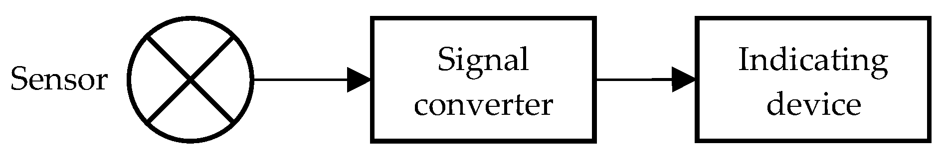
2.1. Displacement Water Meters

Volumetric water meters are measurement devices in which the water flowing through the meter moves the mechanical parts in a cyclical motion [6]. Cyclical motion is continuous motion that, excluding leakage, defines a biunivocal relationship between the volume and position of the moving mechanical parts. Figure 1 illustrates the main elements that compose the measurement chain of the instrument.

The kinematic mechanical chain transforms the movement of the sensor’s moving parts into transmission shaft rotation. Usually, one shaft revolution equals the cyclic volume. The shaft transmits motion to a mechanical converter consisting of a gear box with a constant reduction ratio that converts (N) shaft revolutions into (K) volume divisions and moves forward the figures on a drum indicator accordingly. The kinematic chain of mechanical transmissions of this type of instrument guarantees the continuity of volume metering over time. In addition, the measured volume matches, in the absence of leakage, the actual volume flowing through the instrument, regardless of flow rate variations over time.

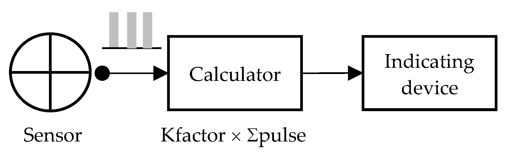
2.2. Turbine Volumetric Water Meter (Velocity Meters)

These meters are manufactured in single-jet and multiple-jet and Woltmann-type turbine meters [6]. For these meters, the water flowing through drives an impeller into rotation with an angular velocity that is a function of the actual flow rate [6,7,8]. In fully mechanical instruments, the turbine’s rotation is transmitted to a gear box, which moves the digits of a drum-type volume indicator. Some types of turbine water meters, such as Woltmann meters, may have an electronic display instead a mechanical indicator. Figure 2 shows a block diagram of a turbine meter with a proximity sensor, being generally inductive (pickup). The sensor generates an electrical impulse when it detects the passage of the turbine blade. The impulse is then acquired and elaborated by an electronic device, which calculates and displays the totalized volume.

The dynamic behavior of mechanical water meters can be examined using a lumped parameter dynamic model [7,8]. The momentum law applied to the mechanical system consisting of an impeller and moving parts provides the mathematical model of Equation (1), where the impeller rotation angle ϕ represents the Lagrange coordinate of the system.

∑T = K_I dω_ϕ/dt

(1)

where ∑T is the sum of all the torques acting on the turbine, K_I is the turbine’s axial moment of inertia and ω_ϕ = dϕ/dt is the turbine’s angular velocity. In a simplified model, it is possible to assume that the sum of the torques acting on the turbine [8] is due to driving torque T_idr exerted by the fluid on the turbine blades and to viscous friction torque T_µ = −K_µω_ϕ. The dynamic equation therefore takes the form of Equation (2).

K_I dω_ϕ/dt + K_μ ω_ϕ = T_idr

(2)

The motion is described by a first-order differential equation into variable ω_ϕ. In fully mechanical meters, the volume indication increases continuously and proportionally to the angle ϕ of turbine rotation. This also applies to instruments equipped with an electronic indicator, where the information is quantized in a discrete pulse signal. Each pulse is the volume integral performed continuously between one pulse and the next one.

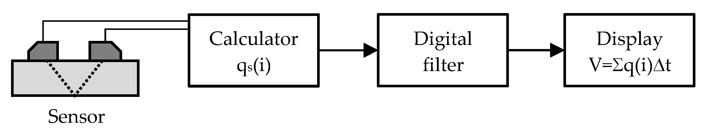
2.3. Ultrasonic Water Meter (Velocity Meters)

Ultrasonic technology is widely used in industry. The measurement principle consists in measuring the transit time of acoustic waves propagating through the moving liquid [6,9]. In water supply systems, ultrasonic measurement technology has been widely used in recent decades due to the development of internal battery-powered meters. This allows the installation of these instruments even in measurement points without mains power, guaranteeing operation for a sufficient lifetime.

Figure 3 shows a simplified block diagram of an ultrasonic water meter’s measurement chain. The signals are processed by the calculator, which provides the measurement of the instantaneous flow rate q_s(i). The sequence of acquired flow rate samples is usually filtered with digital filtering techniques that approximate the behavior of analogue-type filters (IIR, low-pass filter) [10,11]. The digital filtered output value q(i) is used for volume calculation as a discrete sum of finite partial volumes V = ∑q(i)Δt. The flow rate measurement is technically instantaneous, as the cycle time takes just few milliseconds to measure the time difference of the acoustic wave through the liquid. This cycle is repeated at regular intervals, which may vary from a few tens of milliseconds to tens of seconds depending on the construction of the instrument and its sampling settings. For water supply applications, the sampling rate of meters available on the market is around one sample per second [3].

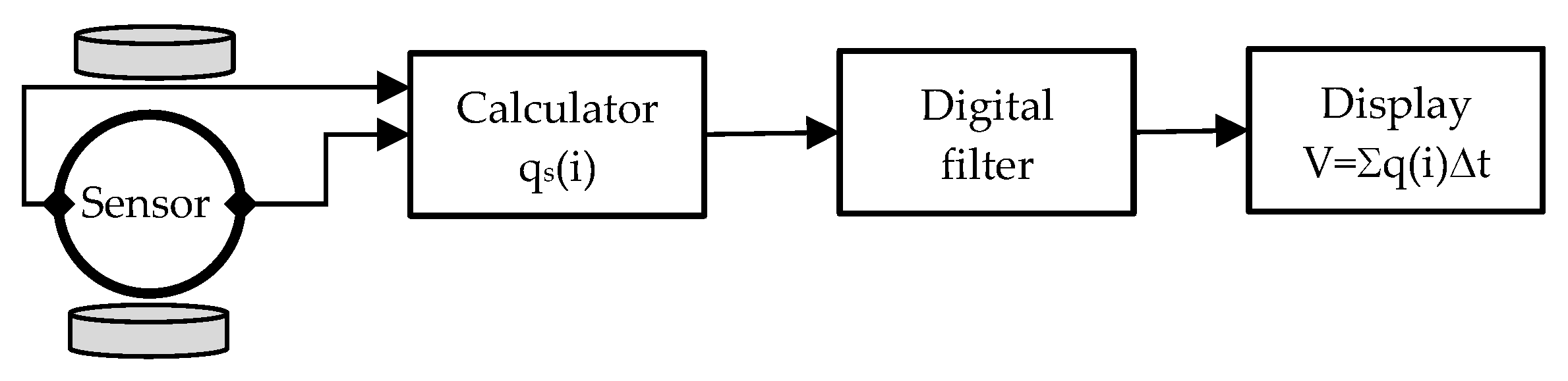
2.4. Electromagnetic Water Meter (Velocity Meters)

Electromagnetic measurement technology, as with ultrasonic measurement technology, is widely used and well known in both the industrial and water supply areas. The measurement principle consists of the measurement of the induced voltage by the moving fluid passing through a magnetic field [12,13]. The generated magnetic field is alternating so as to avoid electrode polarization and to reduce the DC component in the measured signal.

Figure 4 illustrates a simplified block diagram of the measurement chain of electromagnetic water meters. These instruments are equipped with an electronic calculator unit that manages the entire measuring cycle, generates the magnetic field and acquires the signal at the electrodes that are placed in contact with the liquid. The electrical signal is proportional to the mean velocity and, due to the flow sensor geometry, to the volume flow rate [13]. The measurement cycle normally consists of two phases in which the magnetic field direction is reversed. The amplitudes of the electrode signal in the first and in the second phase are compared to provide a flow rate value q_s(i). As for ultrasonic water meters, the acquired flow rate samples are usually filtered by digital filters. The filtered flow rate value q(i) is then used for volume calculation via the discrete sum of finite volumes V = ∑q(i)Δt. Flow rate measurement, similarly to what has been examined for the ultrasonic meter, can be considered technically instantaneous, since the time cycle of magnetic field inversion is usually of the order of tens of milliseconds. Therefore, the electromagnetic water meter samples the flow rate q_w(t) at the magnetic field reversing frequency. For mains-powered instruments, the sampling frequency is a process with several measurement cycles per second. If the electromagnetic water meter is powered by a battery, the measurement cycle is of the order of once per second, in order to ensure a sufficient service lifetime.

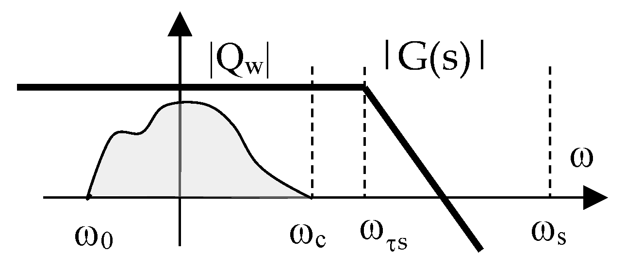
3. Dynamic Response of Continuous-Time Water Meter

The dynamic model of an ideal continuous-time water meter can be described with the block diagrams in Figure 5.

In the time domain, q_w(t) is the volume flow rate at the input of the dynamic system and q(t) is the volume flow rate that the instrument provides at the output. The volume entering the system is the integral over time of the volume flow rate that passes through the meter V_w = ∑q_w(t)dt. In the same way, the volume totalized by the instrument is the integral over time of measured volume flow rate V = ∑q(t)dt. Equation (3) shows the first-order differential equation with time-constant coefficient τ_. This equation represents the simplified dynamic model of continuous-time water meters of Equation (2) [10].

τ dq/dt + q = q_w

(3)

The analysis of the water meter’s dynamic response can also be done in the frequency domain in complex variable s = jω. The block diagram of Figure 5a takes the form shown in Figure 5b, where the Laplace transform is applied to the differential Equation (3). The transfer function G(s) = Q(s)/Q_w(s) [6,10] is the ratio between the transform of output function Q(s) and input function Q_w(s) and takes the form of Equation (4).

G(s) = 1/(1 + τs)

(4)

The transfer function of the first-order linear Equation (4) is a characteristic passive low-pass filter, with a pole in s = −1/τ corresponding to a ω_τ = 1/τ upper cut-off frequency. The meter bandwidth is the frequency interval B_ω = [0; ω_τ]. The cut-off frequency ω_τ = 1/τ depends only on the water meter’s mechanical properties—in particular, the inertia of moving parts. Water meters are instruments designed and manufactured for stationary use, so the dynamic aspects are still little known and often not included in the technical specifications for instruments available on the market. Water meters can measure within the passband B_ω = [0; ω_τ]. Within this frequency interval, the meter elaborates the input to give the output measure. In other words, the passband B_ω = [0; ω_τ] identifies the dynamic meter measuring capability.

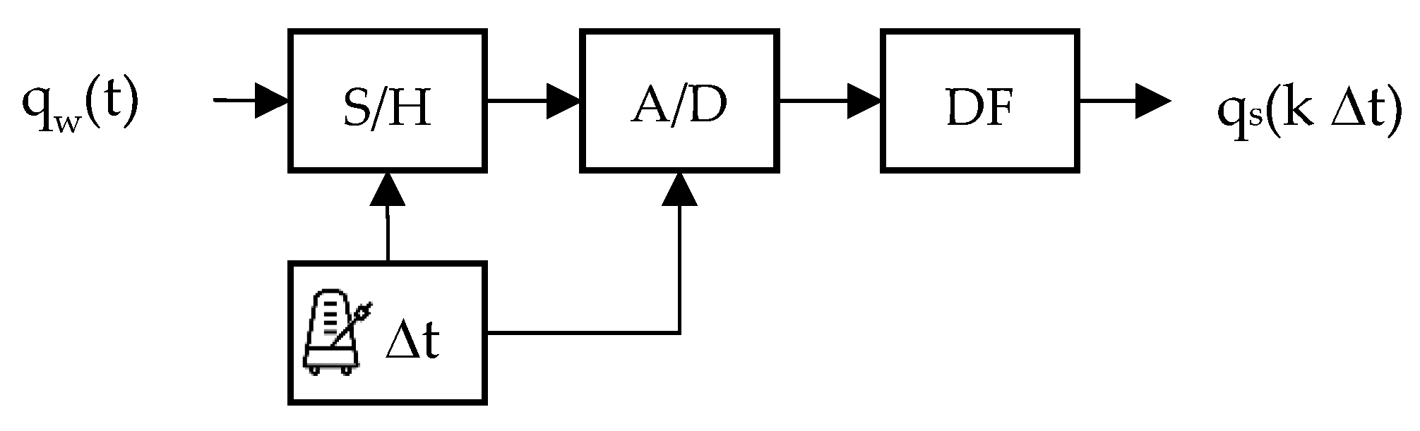
4. Dynamic Response of Discrete-Time Water Meter

Discrete-time water meters are instruments equipped with a calculator unit, where an analogue measurement signal is converted into a digital signal. Figure 6 is not representative of the actual architecture of meters available on the market, but it represents the most significant logic blocks.

The Sample and Hold (S/H) analogue circuit [10] transforms the continuous measurement signal q_w(t) into a discrete analogue signal. The discrete analogue signal is converted into a digital signal by the A/D converter. The analogue-to-digital conversion process involves the discretization of the analogue signal into 2ⁿ discrete levels, where (n) is the number of bits of the A/D converter [10]. The digitalized information is then processed numerically by digital filters to obtain the measured flowrate q_s(k Δt). The calculator performs the volume calculation as the sum of discrete volumes, as shown in Equation (5).

V_s(k Δt) = Δt ∑q_s(k Δt)

(5)

Signal sampling is the key function that impacts the whole measurement process. The measurement cycle Δt is determined by the timing of the circuit board and is at least equal to the time required by the A/D converter to convert the analogue signal into the corresponding digital signal. In general, the sampling time Δt is a selectable parameter and has a direct impact on the power consumption of the board. For each cycle, the electronic board requires a certain amount of energy to acquire, digitalize and process the data. As a consequence, the higher the sampling rate f_s = 1/Δt, the higher will be the required amount of energy. The sampling rate is relevant for battery-powered water meters, where consumption must be proportionate to the battery capacity to obtain a sufficient lifetime. During sample time Δt, the sampled signal is held at the A/D converter input even if the flow rate q_w(t) can vary considerably. This is not a negligible detail, since, in discrete-time systems, sampling allows one to obtain only a part of the information contained in the continuous-time analogue signal. Intuitively, it is possible to increase the information content by increasing the sampling rate f_s = 1/Δt. The criteria to determine the appropriate sampling rate are defined by sampling theorem. The following is one of the formulations available in the literature [10]: “If a continuous, bandwidth-limited signal contains no frequency components higher than f_c, then the original signal can be recovered without distortion if it is sampled at a rate of at least f_s > 2f_c samples per second.”

The sampling theorem serves as a fundamental bridge between continuous-time signals and discrete-time signals and establishes a sufficient condition for capturing all the information from a continuous-time signal by sampling. Moreover, for discrete-time water meters (ultrasonic and magnetic), the analogue measurement signal is generated at the same time as sampling, without the ability to apply a filter to the whole input signal q_w(t) to limit its bandwidth. This condition permits folding and aliasing phenomena, which can be limited only by increasing the sampling rate [10]. The optimal working conditions are shown in Figure 7, where the q_w(t) input signal bandwidth is limited, B_c = [ω₀, ω_c], and the sampling rate ω_s = 2πf_s satisfies the sampling theorem ω_s > 2ω_c.

The sampling theorem ω_s/ω_c > 2 is met by assuming an adequate margin, which is at least ω_s/ω_c > 2.5 [11] or more commonly ω_s/ω_c > 10 [10]. This permits the acquisition of a sufficient amount of information to obtain a dynamic response congruent to the input flow rate.

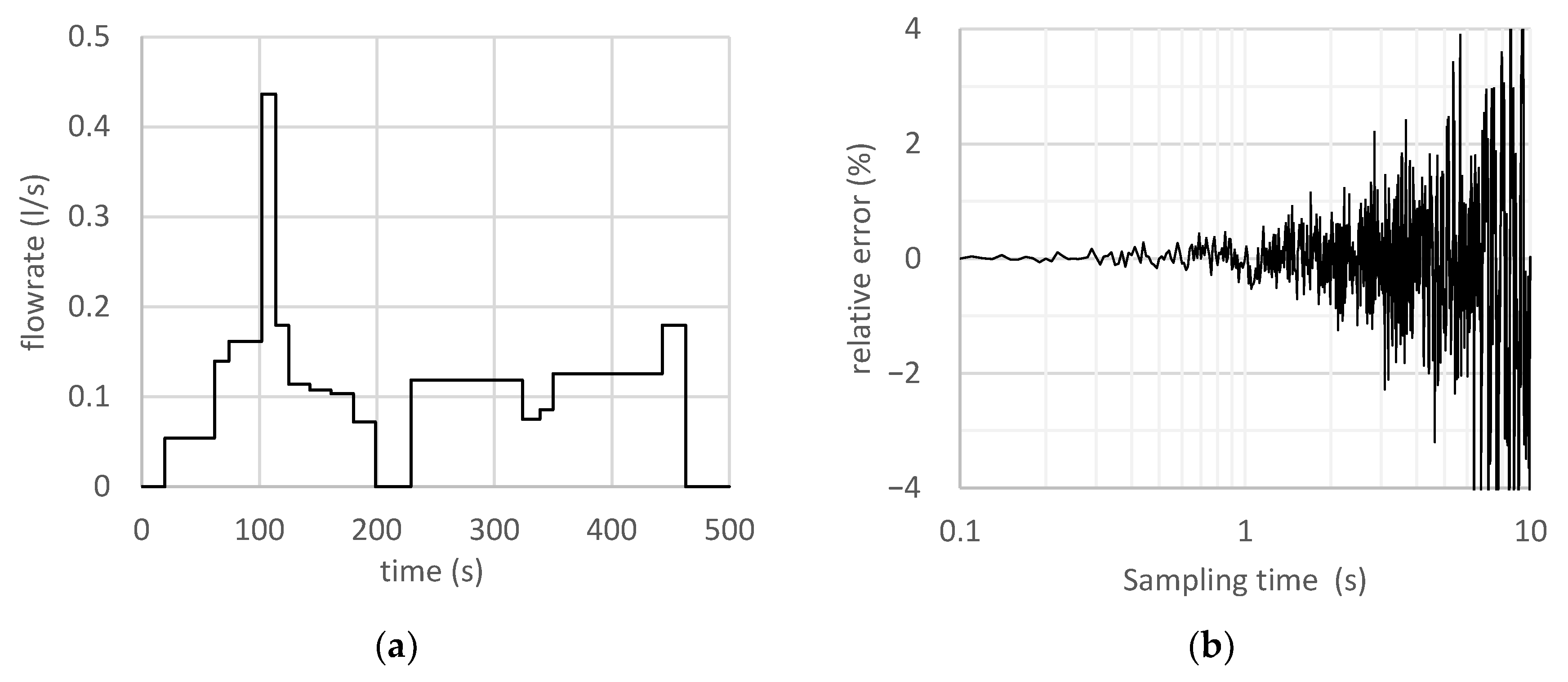
5. Measurement Error and Sampling Rate

For discrete-time volume meters, the effect of sampling on volume measurement accuracy can be examined in detail. Among the consumption profiles available in the literature, the dynamic consumption profile shown in Figure 8a is examined [4].

The dynamic profile has a total duration of 500 s and is characterized by a variable flow rate in the range from 0.00 L/s up to around 0.45 L/s. Total volume is equal to V_ref = 51.455 l.

To evaluate the effect of sampling on volume counting, the flow profile in Figure 8a is numerically sampled with sampling time Δt (s) rising from Δt_min = 0.1 s to Δt_max = 10 s with step Δt = 0.1 s. For each sampling time Δt, the volume V_s. = f(Δt) is calculated as the sum of discrete volumes equal to the flow rate q_s(kΔt) sampled at time t(k) = k Δt multiplied by the time Δt, as shown in Equation (5). The volume counting error is determined for each sampling time Δt according to Equation (6).

E = (V_s − V_ref)/V_ref × 100

(6)

The percentage error values are shown in Figure 8b as a function of sampling time Δt. Analysis of the graph shows that the counting error is relatively small for sampling times less than approximately Δt ≤ 1 s. The counting error increases rapidly for sampling times greater than Δt > 1 s. Discrete-time volume counters that meet the stationary error limits [1] for accuracy classes 1 and 2 may not meet the error limits under dynamic operating conditions. With reference to the dynamic flow profile of Figure 8a, it can be observed that to comply with the error limits for class 1 (MPE ≤ 1%), the sampling time must be less than Δt < 2 s. Similarly, to comply with the maximum error limits allowed for class 2 (MPE ≤ 2%), the sampling time must be less than Δt < 3 s. Referring to the relationship between sampling time Δt and compliance with maximum permissible errors, the observations are valid only for the flow profile of Figure 8a. With other flow profiles, the conclusions may be different.

6. Dynamic Response, Classification and Test Methods

The water meter’s dynamic response is currently under investigation. In general, the most relevant aspect of the dynamic response is the responsiveness and rapidity with which the instrument can reproduce the measured quantity fluctuations. Some of the characteristics of water meters are already expressed in classes [1]—for example, accuracy classes, temperature classes or hydraulic profile sensitivity classes. Classes allow the manufacturer to concisely provide the user with detailed information about the instrument. Still missing from this information is the meter’s dynamic response, which can be expressed in several equivalent ways. The most general expression is the measuring bandwidth [ω_min, ω_max]. The information, expressed as a range of frequencies, is easily divided into classes, where the maximum frequency identifies the instruments that have greater responsiveness. From an application field point of view, the information expressed as frequency intervals may not be easy to use. The technical approach is most familiar with the expression of the time constant τ. The time constant allows an immediate comparison of dynamic performance; the smaller the time constant, the faster the instrument’s response. From this perspective, classification in terms of time constant [τ_min, τ_max] is more desirable. However, it should be noted that the expression of dynamic performance in terms of time constant blinds the meter to a first-order linear dynamic model. This is a strong limitation to the development and implementation of innovative measurement systems. To investigate the dynamic response and regulate dynamic requirements of water meters, it is necessary to develop standardized methods so that the accredited laboratories can perform testing according to common and defined rules [14]. The most effective strategy is to define dynamic test methods that can be executed on common test facilities equipped for stationary conditions, requiring limited changes to the actual facility and metrological reference structure. In this way, the standard step response can be identified as the test method of immediate application [8]. In practice, it is possible to intercept the flow with a valve and proceed with rapid openings and closures to evaluate the resulting transient water meter response.

The main limitations using this approach are the speeds of the opening and closing of the shut-off valve: the speed must be carefully evaluated according to the expected performance of the water meter under test and to the test facility’s dynamic operating conditions to avoid water hammer phenomena. A second approach to limit, or even completely eliminate, the water hammer phenomena is a test method that provides a sinusoidal flow rate of defined amplitude and frequency [7,8]. A first-order water meter provides a sinusoidal flow rate of attenuated amplitude and a time-delayed response. This method requires, as a step response method, the interception of the flow with a valve that can modulate the flow, realizing a sinusoidal flow profile. Both approaches require minimal arrangements in existing facilities and the management of the metrological traceability of time as an additional quantity.

7. Conclusions

The dynamic behavior of mechanical water meters can be analytically approximated by a first-order linear differential equation. The corresponding transfer function G(s) = 1/(1 + τs) in the complex domain depends on a single parameter having the size of a time constant τ. Discrete-time water meters, such as ultrasonic and electromagnetic ones, have dynamic behavior, which can be related to mechanical water meters if the sampling theorem is fulfilled and if the water meter calculator implements digital filters simulating first-order analogue filters with time constant τ. A general criterion for dynamic response classification is the water meter’s bandwidth [f_min, f_max]. A more user-friendly classification criterion is the time constant [τ_min, τ_max], where the smaller is the time constant, the more responsive is the water meter. A classification according to this criterion is less general than the bandwidth because it always assumes a first-order linear dynamic model of equations. Test methods for water meters’ dynamic responses are under study and there are no standardized methods yet available. The lack of standardized test methods is the major obstacle, because test laboratories do not have a well-proven technical basis for implementing a metrologically traceable test facility. Two test methods, which are easy to implement in testing and calibration laboratories, were examined. Both refer to the standard step and sine responses. The step response method has technical limitations due to the rapidity of the opening and closing operations of the shut-off valve, which must be carefully evaluated in order to avoid water hammer phenomena. The sinusoidal flow rate response is a test method that allows one to limit water hammer effects. The repetition of the sinusoidal flow rate test at different frequencies allows the experimental determination of the water meter response spectrum.

References

1. OIML R 49-1:2013. Available online: https://www.oiml.org/en/files/pdf_r/r049-1-e13.pdf (accessed on 21 April 2022).
2. ISO 4064-1:2014. Available online: https://www.iso.org/standard/55371.html (accessed on 21 April 2022).
3. Schumann, D.; Kroner, C.; Unsal, B.; Haack, S.; Kondrup, J.B.; Christophersen, N.; Benkova, M.; Knotek, S. Measurements of water consumption for the development of new test regimes for domestic water meters. Flow Meas. Instrum. 2021, 79, 101963. [Google Scholar] [CrossRef]
4. Büker, O.; Stolt, K.; Lindström, K.; Wennergren, P.; Penttinen, O.; Mattias son, K. A unique test facility for calibration of domestic flow meters under dynamic flow conditions. Flow Meas. Instrum. 2021, 79, 101934. [Google Scholar] [CrossRef]
5. ISO4006:1991. Available online: https://www.iso.org/standard/9681.html (accessed on 21 April 2022).
6. Sydenham, P.H. Handbook of Measurement Science, Volume 2: Practical Fundamentals, 5th ed.; Wiley: Oxford, UK, 1997; ISBN 0-471-10493-0. [Google Scholar]
7. Lee, B.; Cheesewright, R.; Clark, C. The dynamic response of small turbine flowmeters in liquid flows. Flow Meas. Instrum. 2004, 15, 239–248. [Google Scholar] [CrossRef]
8. Yuan, Y.; Zhang, T. Research on the dynamic characteristics of a turbine flow meter. Flow Meas. Instrum. 2017, 55, 59–66. [Google Scholar] [CrossRef]
9. ISO12242:2012. Available online: https://www.iso.org/standard/51289.html (accessed on 21 April 2022).
10. Sydenham, P.H. Handbook of Measurement Science, Volume 1: Theoretical Fundamentals, 1st ed.; Wiley: Oxford, UK, 1982; ISBN 0-471-10037-4. [Google Scholar]
11. Bose, N.K. Digital Filters: Theory and Applications, 1st ed.; North-Holland, Elsevier Science Publishing Co., Inc.: New York, NY, USA, 1985; ISBN 0-444-00980-9. [Google Scholar]
12. ISO 20456:2017. Available online: https://www.iso.org/standard/68092.html (accessed on 21 April 2022).
13. Shercliff, J.A. The Theory of Electromagnetic Flow-Measurement, 2nd ed.; Cambridge University Press: Cambridge, UK, 1987; ISBN 0-521-33554-X. [Google Scholar]
14. ISO/IEC 17025:2017. Available online: https://www.iso.org/standard/66912.html (accessed on 21 April 2022).
Figure 1. Displacement water meter measurement chain.
Environsciproc 21 00031 g001
Figure 2. Turbine water meter measurement chain.
Environsciproc 21 00031 g002
Figure 3. Ultrasonic water meter measurement chain.
Environsciproc 21 00031 g003
Figure 4. Electromagnetic water meter measurement chain.
Environsciproc 21 00031 g004
Figure 5. Continuous water meter dynamic model: (a) time domain; (b) frequency domain.
Environsciproc 21 00031 g005
Figure 6. Dynamic model of discrete-time water meter.
Environsciproc 21 00031 g006
Figure 7. Flow rate Qw(s) with bandwidth Bc = [ω0, ωc] coupled to water meter with sampling rate ωs > 2ωc and meter passband Bω = [0; ωτs]. (The figure is plotted on bi-logarithmic axes.)
Environsciproc 21 00031 g007
Figure 8. Dynamic flow profile and totalized volume relative error function due to sampling time: (a) dynamic flow profile; (b) volume counting error due to sampling time varying from Δt = 0.1 s to Δt = 10 s at Δt step of 0.1 s.
Environsciproc 21 00031 g008
Publisher’s Note: MDPI stays neutral with regard to jurisdictional claims in published maps and institutional affiliations.