Abstract
To provide quantitative elements to the expected rate of change of flood quantiles in Alpine basins due to global warming, a systematical assessment of a river network is undertaken in this paper through the implementation of a geomorphoclimatic approach. The model, called “FloodAlp” produces the flood frequency curve of mountainous catchments based on the stochastic interaction of precipitation and temperature. In view of a widespread application, FloodAlp was revamped here and applied to all the sections of the river network of the Chisone basin (Northwest Italy) identified through a 50 m resolution digital elevation model (DEM). We show that, based on the decrease in snow-affected contributing areas, flood frequency can increase up to 8 times compared to the current frequency, with amplifications depending on the local elevation characteristics of sub-basins.
1. Introduction
The increasing temperatures that have been observed in the last several decades inevitably affect the natural processes causing floods in the mountains, where the snow dynamics largely influence the timing and volumes of runoff [1,2,3]. Mountain hydrological processes have been taken under special consideration in the scenarios deriving from future climate conditions, even though flood risk management has not yet received all the necessary attention. In fact, several studies on this topic concern the earlier snow melting and variation in spring flood peaks (see, e.g., the work of Shea et al. [4]), with consequent variations in runoff seasonality (see, e.g., the work of Schneeberger et al. [5]). Processes occurring in mountainous regions significantly vary in space, as they strongly depend on the high spatial variability in altitude, slope and aspect in the involved watersheds [6]. In this work, we address the question of how the heterogeneity due to the elevation features is involved in modifying the magnitude and frequency of flood events under global warming.
The model application presented here is not intended to address the probabilistic assessment of flood quantiles for a given return period but deals with the evaluation of the rate of change of a given flood quantile as a consequence of temperature (and precipitation) increase scenarios. Here we use the FloodAlp model [7], which is based on a derived distribution approach. The model produces a simplified flood frequency curve based on the annual variation of the portion of the basin covered by snow, according to how the seasonal variation of the freezing elevation affects the hypsographic curve of the basin.
The rationale behind the FloodAlp model is to try to simplify as much as possible the elements that can produce variations in the flood-forming conditions in Alpine basins, so to help in discriminating, in a wide-area context, how the intensification of flood frequency changes among different river sections solely based on topography.
The contribution of the present work follows two directions. On the one hand, the FloodAlp model is explicitly implemented over different river basins for the first time. This provides feedback on its capability to capture the form of the flood frequency curve in snow-driven watersheds. The second objective is to show how the estimated relative entity of flood increments due to climate change can vary heavily in space. This is addressed using a high-resolution digital elevation model and can be of interest to scientists and practitioners.
The application is systematically carried out along the stream network of the Chisone basin, located in the northwestern portion of the Piedmont region (Italy) and characterized by geomorphoclimatic features that are reasonably representative of the Italian Alpine watersheds.
The minimal data requirement of the FloodAlp model, described below, indicates that the approach is intended to provide a tool that in a rapid but straightforward way can help in discriminating basins in relation to the possible increase in flood frequency. This classification, valid for mountainous, snow-affected areas, is essentially based on the variability of the basin elevation features, all the other elements being equal (i.e., rainfall extremes statistics and average annual rainfall).
2. Materials and Methods
2.1. The FloodAlp Model
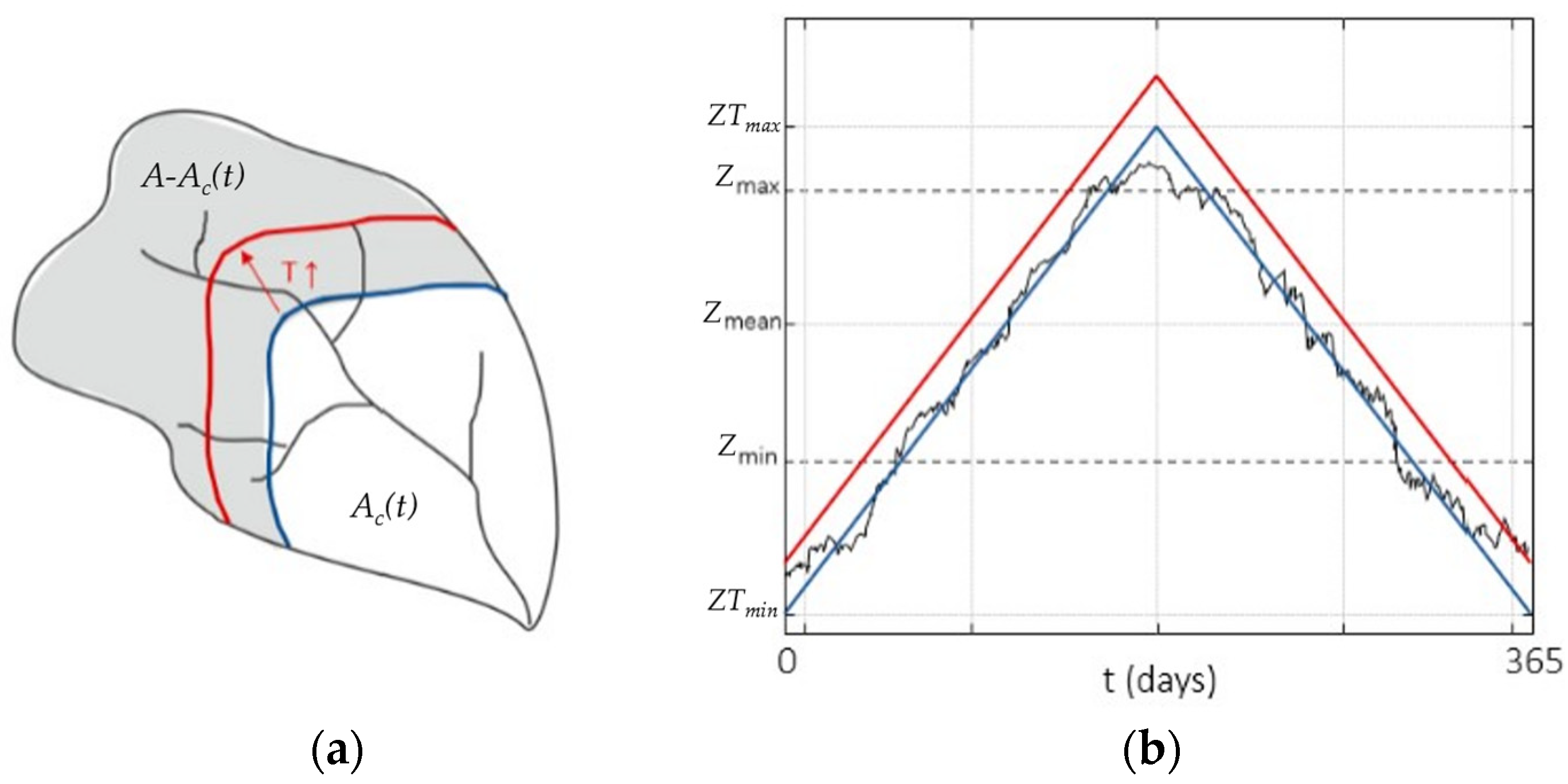
The FloodAlp model [7] operates on the relationship between flood formation and the basin elevation distribution when in a precipitation event only a portion of the basin can be considered “active”. This portion, called the “contributing area” (Ac(t)), is the one that receives liquid precipitation and lies below the freezing elevation (Figure 1). As sketched in Figure 1a, the freezing elevation identifies the contour line above which temperatures are below zero, such that the precipitation falls as snow. In average terms, the freezing elevation ZT(t) is seasonal, as it varies with the thermal regime of an area. In the model, a linear symmetric curve (Figure 1b) is used to describe its variability over time. Because of this time variability, the areal reduction factor fc(t) = Ac(t)/A varies over time. The quantitative variability of fc(t) depends on the basin hypsometry, and here resides the influence of topography in the flood generation mechanism.
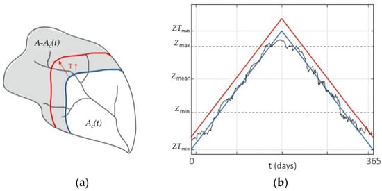
Figure 1.
Schematic representation of the model concept: as a function of the freezing elevation ZT(t) on the day t, the relevant contour line delimitates the contributing area Ac(t) on the same day (a). In (b), the blue line represents the freezing elevation annual regime. In both panels, the red line exemplifies the result of a temperature increase.
The model considers runoff as the sum of the precipitation affecting the contributing area and a snowmelt component SM, according to the following relation:
where q is the specific discharge (mm/h), C is the peak runoff coefficient (-), h is the rainfall depth (mm) and t is the Julian date (days). SM(t) is a deterministic component added to account for the snow melting contribution during the warm season. SM(t) is assumed to be zero in the cold season and variable during the warm season.
The rainfall process is modeled according to a Poisson representation of storm arrivals in time, with rate λ, each storm having a depth h which is an exponentially distributed random variable with mean α. The rainfall duration considered for h is 24 h. To preserve the units, q is a specific daily average discharge, evaluated in mm/h. Starting from the probability distribution of the rainfall, the distribution of extreme floods is derived in a closed analytical form in the work of Allamano et al. [7].
In view of a systematic model application, the parameters required are as follows:
- the freezing-curve boundaries: ZTmax and ZTmin;
- a parameter controlling the flexure of the hypsometric curve, hereinafter referred to as ζ, as well as the maximum and minimum basin elevations;
- the total annual average areal precipitation which, together with the areal reduction factor, is used to estimate SM(t);
- the parameters of the rainfall model α and λ.
2.2. Study Area
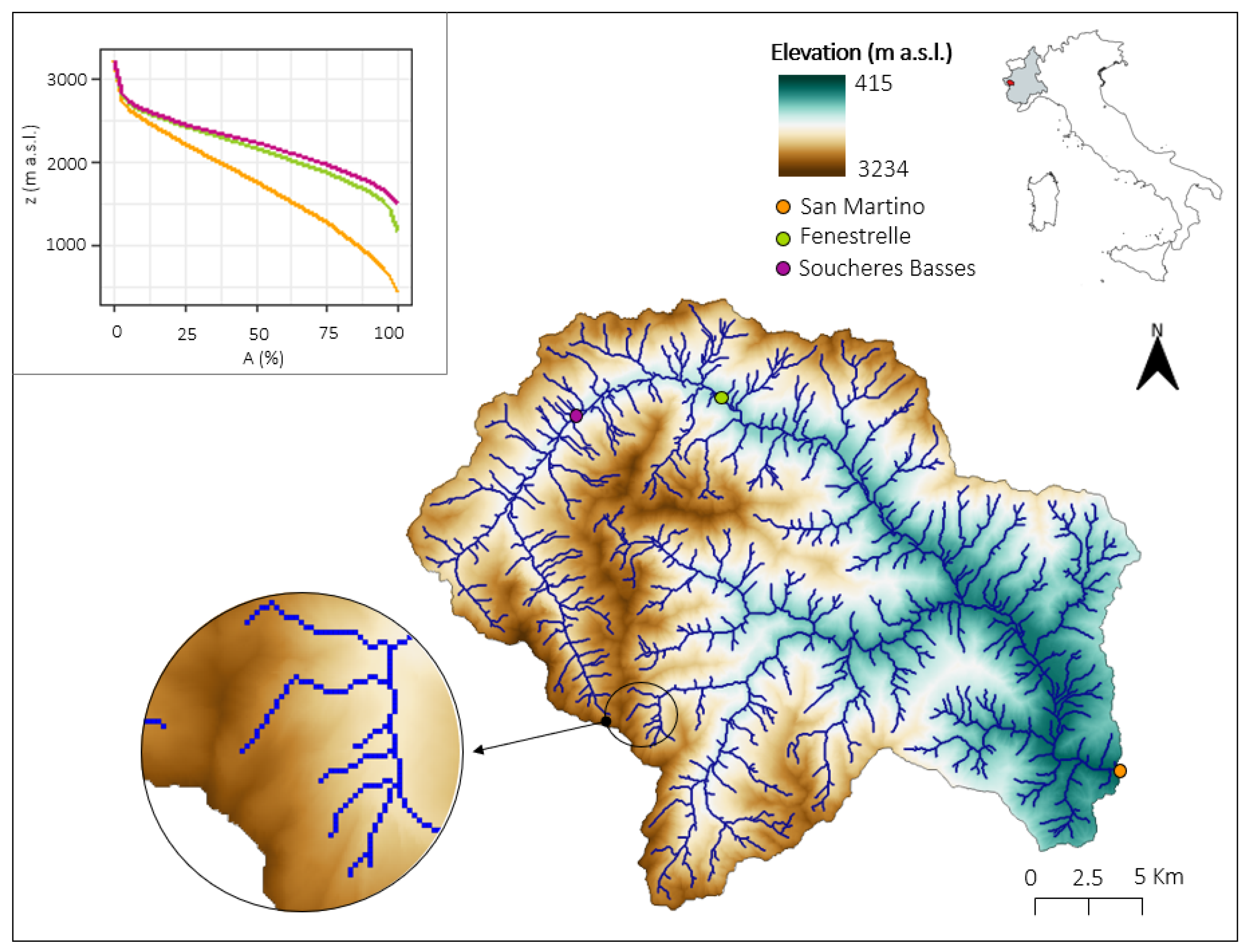
This study is focused on the Chisone basin, an Alpine watershed located in the western part of the Piedmont region in Italy (Figure 2). The basin area is 580 km2, and its elevation ranges from 415 to 3234 m a.s.l.
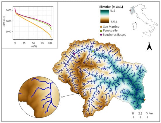
Figure 2.
River network of the Chisone basin having its outlet in San Martino (orange dot). Two other gauged sections within the basin, Fenestrelle and Soucheres Basses, are indicated with a green and a purple dot, respectively. The top left graph shows the hypsographic curves of the three basins with normalized areas on the x-axis.
The river network of the investigated basin was extracted from a digital elevation model (DEM) at a 50 m spatial resolution, partly processed in the Renerfor project [8]. This resolution was maintained for the selection of over 12,000 sections, all referring to the respective sub-basins. The analyses were applied to all the sections of the river network within the basin, moving along the streams progressively with a 50 m step. In the network definition, an area threshold of 0.25 km2 for channel initiation was used.
For all the 12,474 pixels belonging to the river network, we derived the parameters of the FloodAlp model using available climatic maps and interpolation. In further detail, based on what was suggested by Allamano et al. [7], the freezing elevation was assumed to range between ZTmin = 0 m a.s.l. and ZTmax = 3000 m a.s.l. The distribution of the elevations is summarized by the minimum and maximum elevations, and by the ζ flexure parameter (see the work of Allamano et al. [7]). For each of the 12,474 sub-basins, ζ was computed by equating the integral of the hypsometric curve with the normalized mean elevation of each sub-basin.
The total annual average precipitation was calculated by processing monthly mean rainfall maps available in the work of Braca et al. [9], while the parameters of the rainfall model were computed from maps of Gumbel extreme rainfall statistics produced as part of the STRADA project [10] at a 250 m spatial resolution. The α and λ parameters were thus computed as follows:
where and are the parameters of the Gumbel distribution [11].
2.3. Model Application
To assess the FloodAlp model performance in predicting the flood frequency distribution, the model was applied to three gauged sections, where the annual maxima of the daily average discharge are available, i.e., the Chisone at Soucheres Basses, Chisone at Fenestrelle and Chisone at San Martino.
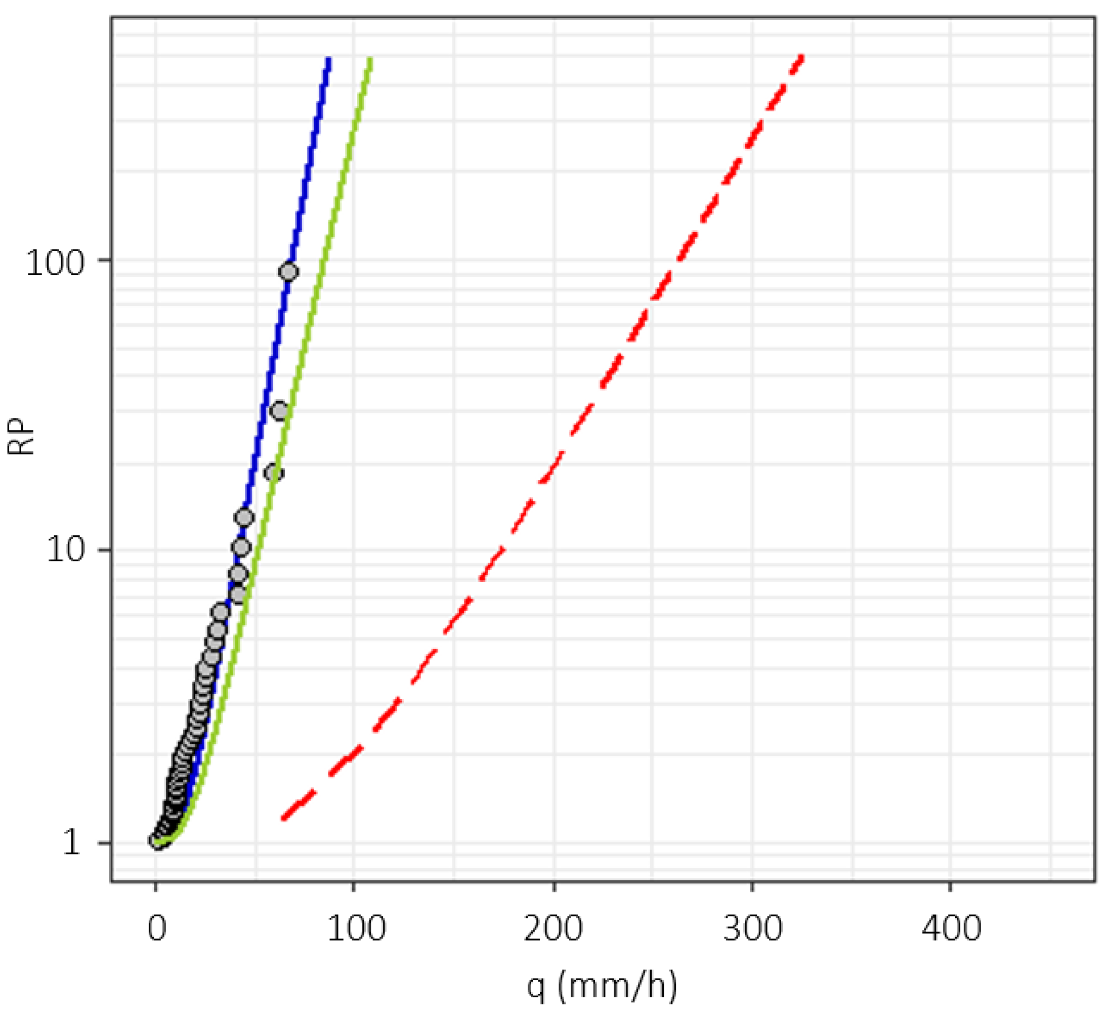
The application of the model for the Chisone basin in San Martino is detailed in Figure 3 (very similar results have been obtained for the other stations). The blue curve is the frequency curve deriving from the model application under current climate conditions, while the grey dots represent the daily annual discharge maxima, retrieved from the Catalogo delle Piene dei Corsi d’acqua Italiani [12]. To obtain the model curve, the runoff coefficient in Equation (1) was calibrated to fit the maximum observed historical discharge, resulting in C = 0.43. The dashed red line is the Gumbel rainfall frequency curve, corresponding to a hypothetical flood frequency distribution which would derive from assuming C = 1 and that no attenuation of flood quantiles derives from the partial contributing area effect due to snow [7]. This comparison shows separately the shifts of the rainfall curve due to the runoff coefficient value and the partial contributing area effect.
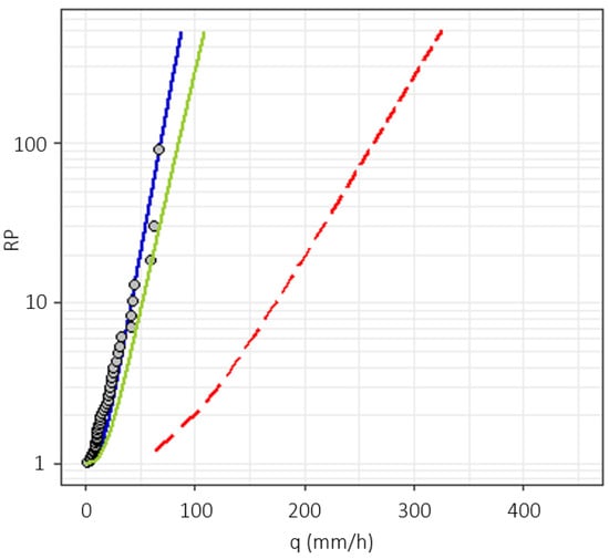
Figure 3.
Example of flood mitigation induced by snow modeled with FloodAlp for the Chisone basin. The blue and green lines are the flood frequency distributions under current andperturbed climatic conditions, respectively. Curves are compared to the annual maximum daily discharges observed at the same station. The dashed red line is the Gumbel rainfall frequency distribution.
Due to its structure, FloodAlp can be also applied to verify in which way a displacement of the snowline, caused by a rise in temperature and/or an increase in precipitation, can influence floods with an assigned return period. The application of climatic perturbations produces a rightward-shifted flood frequency distribution, i.e., the green curve in Figure 3. The probability of exceeding a given specific discharge, read on the “future” curve, will differ from the probability of exceeding the same event under present conditions, in a measure that depends on the distance between the two curves.
To meet the goal of assessing the variation in flood frequency distributions, we started by calculating, for each pixel of the Chisone river network, the flood frequency distribution in an “undisturbed” condition, i.e., when no attenuation performed by snow occurs. For each pixel, we then computed, through FloodAlp, the 100-year undisturbed specific discharge q100.
In analogy with the suggestion of Allamano et al. [13], we assessed the effects of change through the return period ratio (RPR) coefficient defined as follows:
where RP is the return period of a flood discharge corresponding to the undisturbed q100 under current climatic conditions (blue curve in Figure 3) while RP’ is the return period of the same discharge under modified climatic conditions (green curve in Figure 3).
To evaluate the effect of climate change on the flood extent, our analytical model was perturbed according to different climate change scenarios, defined as follows:
- Scenario 1: raising of the zero-degree isotherm ZT by 400 m (RPR1), corresponding to a temperature increase of approximately 3 °C;
- Scenario 2: raising of the average rainfall intensity α by 10% (RPR2), following the reasoning of Allamano et al. [13];
- Scenario 3: increase in both temperature and precipitation (RPR3).
As outlined in Section 1, here we also preliminarily investigated the role of the morphological characteristics of sub-basins on the increase in flood frequency due to the reduction in snow-affected contributing areas. Finally, Spearman’s rank correlation coefficient for the return period ratio and the mean and minimum elevations of sub-basins was computed.
3. Results and Discussion
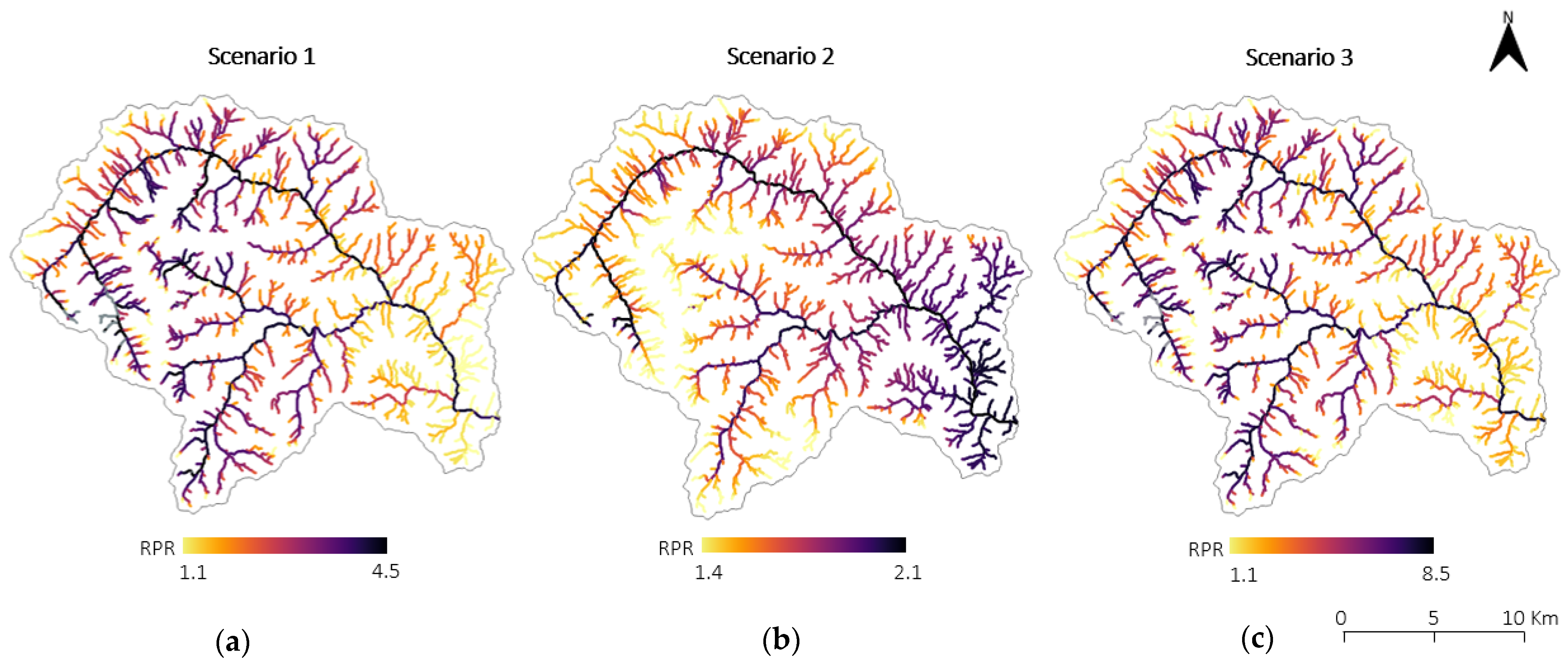
The application of the above-mentioned procedure over the whole Chisone network produced results that can be shown as maps of RPR (Figure 4). Rather than sensitivity to a precipitation increase, a marked sensitivity of the Alpine watersheds to increasing temperatures emerges. The RPR coefficient reaches values up to 8.5 for scenario 3 (Figure 4c).
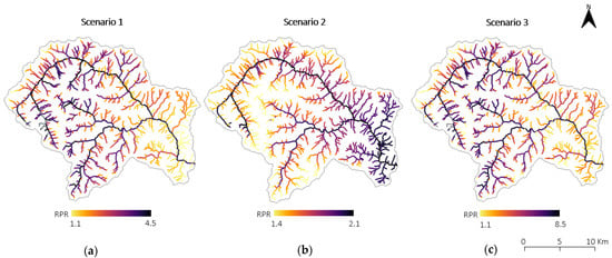
Figure 4.
Variability of the RPR index along the stream network under the hypothesis of ΔZT = 400 m (a), Δα = 10% (b), or ΔZT = 400 m and Δα = 10% (c). Gray points show RPR higher than 4.5 for the first scenario and higher than 8.5 for the third scenario. This occurs in sub-basins having very high minimum elevations.
The RPR1 and RPR3 over the river network show a similar pattern, with a progressive increase for increasing elevations. On the other hand, a decreasing path with elevation can be observed for the RPR2 values (i.e., precipitation increase only). This different, opposite, behavior can be understood by considering that basins having a very high minimum altitude remain almost always above the freezing elevation; for these basins, a change in precipitation does not affect the final flood frequency very much. The lower the basin elevation, the more the increase in α will be reflected in the increase in frequency, as most of the basin area will be contributing to the flood.
Another outcome of this analysis is the fact that in all three cases the RPR values are higher moving along the main channel than along the tributaries; this is due to the mean altitude of the basins drained by the tributaries being lower than the mean elevation of the main basin.
All these findings are consistent with those of Allamano et al. [13].
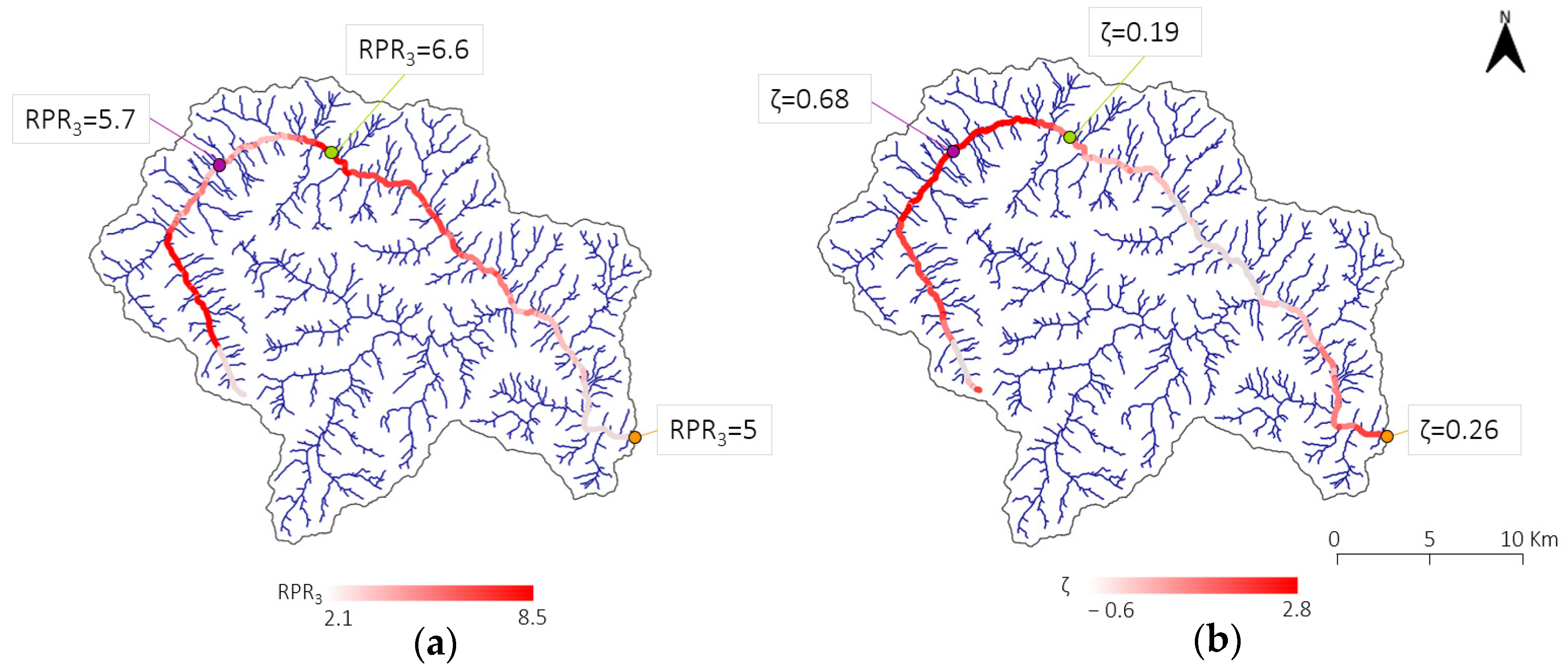
As previously mentioned, we also assessed the link between the RPR index and some basin morphological features, e.g., the ζ parameter. The ζ parameter controls the distribution of areas at different basin elevations, thus representing an important indicator of how much a basin may be affected by significant vertical variations in the position of the snowline. A map describing the variability of ζ along the river network is compared to the map of RPR3 in Figure 5. A rather close relationship between the RPR values and the ζ parameter over the main channel is apparent; the two quantities seem to vary inversely, except for in the last reach of the main channel.

Figure 5.
RPR3 (a) and flexure parameter of the hypsometric curve (b) along the main channel. The values at the three gauged stations are indicated.
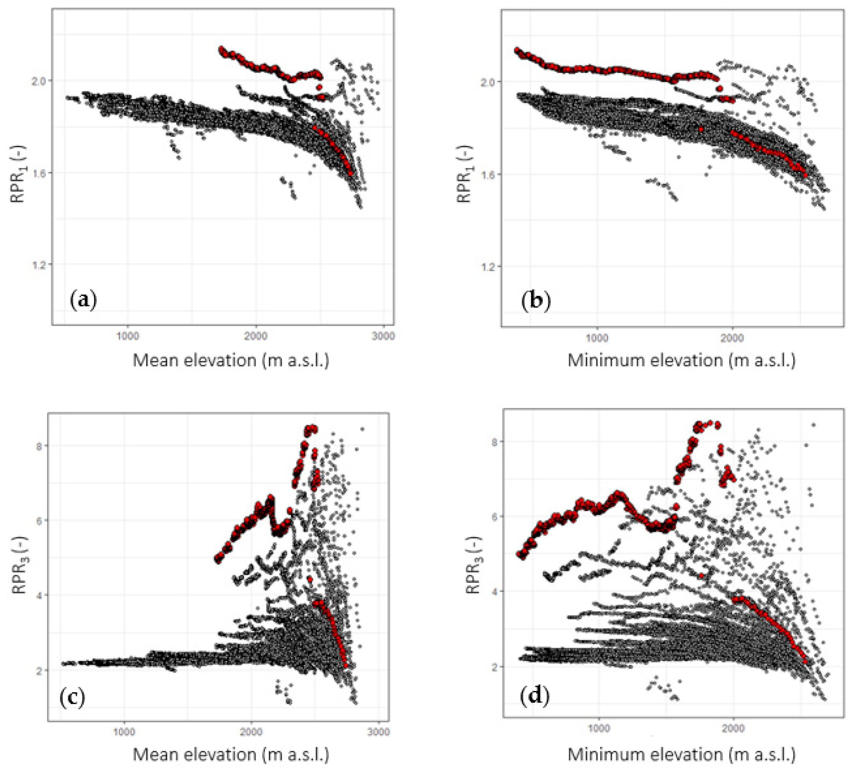
Figure 6 shows the relationship between the RPR values and the mean (Figure 6a,c) and minimum (Figure 6b,d) elevation of the sub-basins for the first (Figure 6a,b) and third (Figure 6c,d) climate change scenarios. Red points represent the main channel.
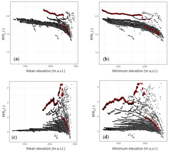
Figure 6.
Scatter plots showing the relationship between the RPR index for two of the described climate scenarios and the altimetric features of the sub-basins. (a,b) Relationship between the RPR1 values and the mean and minimum sub-basin elevations, respectively. (c,d) Relationship between the RPR3 values and the mean and minimum sub-basin elevations, respectively.
While the RPR1 values follow a decreasing pattern with both the minimum and mean basin elevations, the variation of the RPR3 values follows a more complex path. In all cases, a drop in the RPR index can be observed for mean and minimum elevations higher than 2500 m and 2000 m a.s.l., respectively. This is due to the decay of the snow melting contribution (SM(t)) for particularly high-elevation areas. Thus, the ratio between the snowmelt contribution under both current and climate change conditions tends to decrease for very high elevations. Points showing the lowest RPR values are actually those belonging to the last reach of the main channel.
The different behavior shown by RPR1 and RPR3 is confirmed by Spearman’s rank correlation coefficient, which is in the order of −0.95 and 0.42 for scenarios 1 and 3, respectively, for both mean and minimum elevation.
4. Conclusions
In this paper, we applied a simple morphoclimatic flood frequency model aimed at investigating changes in flood risk in Alpine and pre-Alpine areas due to future variations in climatic conditions of temperature and precipitation. The proposed application identifies in a systematic way, section by section on the river network of the Chisone basin, the increase factor of the frequency of an “originary” 100-year flood. This application allows an overall examination of the vulnerability of mountain areas to climate change.
In order to understand how each stream responds to the climatic perturbations implemented in the model, we also provided some comments on how the basin morphological features and the area-elevation distribution may influence this response. This study suggests that further efforts to understand these relationships are certainly needed.
Author Contributions
Conceptualization, P.C., G.E. and I.M.; methodology, P.C., G.E. and I.M.; software, G.E. and I.M.; validation, G.E.; formal analysis, G.E. and I.M.; investigation, G.E. and I.M.; resources, P.C.; data curation, G.E.; writing—original draft preparation, G.E. and I.M.; writing—review and editing, P.C. and G.E.; visualization, G.E.; supervision, P.C.; project administration, P.C.; funding acquisition, P.C. All authors have read and agreed to the published version of the manuscript.
Funding
This research received no external funding.
Institutional Review Board Statement
Not applicable.
Informed Consent Statement
Not applicable.
Conflicts of Interest
The authors declare no conflict of interest.
References
- De Jong, C. Challenges for mountain hydrology in the third millennium. Front. Environ. Sci. 2015, 3, 38. [Google Scholar] [CrossRef]
- Castellarin, A.; Pistocchi, A. An analysis of change in alpine annual maximum discharges: Implications for the selection of design discharges. Hydrol. Process. 2012, 26, 1517–1526. [Google Scholar] [CrossRef]
- Molini, A.; Katul, G.G.; Porporato, A. Maximum discharge from snowmelt in a changing climate. Geophys. Res. Lett. 2011, 38, L05402. [Google Scholar] [CrossRef]
- Shea, J.M.; Whitfield, P.H.; Fang, X.; Pomeroy, J.W. The Role of Basin Geometry in Mountain Snowpack Responses to Climate Change. Front. Water 2021, 3, 604275. [Google Scholar] [CrossRef]
- Schneeberger, K.; Dobler, C.; Huttenlau, M.; Stötter, J. Assessing potential climate change impacts on the seasonality of runoff in an Alpine watershed. J. Water Clim. Chang. 2015, 6, 263–277. [Google Scholar] [CrossRef]
- Tennant, C.J.; Crosby, B.T.; Godsey, S.E. Elevation-dependent responses of streamflow to climate warming. Hydrol. Process. 2015, 29, 991–1001. [Google Scholar] [CrossRef]
- Allamano, P.; Claps, P.; Laio, F. An analytical model of the effects of catchment elevation on the flood frequency distribution. Water Resour. Res. 2009, 45, W01402. [Google Scholar]
- Ganora, D.; Gallo, E.; Laio, F.; Masoero, A.; Claps, P. Analisi Idrologiche e Valutazioni del Potenziale Idroelettrico dei Bacini Piemontesi, Relazione finale del progetto RENERFOR-ALCOTRA, Regione Piemonte. 2013. Available online: http://www.idrologia.polito.it/web2/open-data/Renerfor/analisi_idrologiche_LR.pdf (accessed on 12 March 2022).
- Braca, G.; Bussettini, M.; Lastoria, B.; Mariani, S.; Piva, F. Elaborazioni Modello BIGBANG Versione 4.0, Istituto Superiore Per la Protezione e la Ricerca Ambientale–ISPRA. 2021. Available online: http://groupware.sinanet.isprambiente.it/bigbang-data/library/bigbang40 (accessed on 12 March 2022).
- Claps, P.; Laio, F.; Allamano, P.; Libertino, A.; Iavarone, M. Attività di ricerca nell’ambito del Progetto STRADA 2.0 MODULO CAPPIO. 2015. Available online: http://www.idrologia.polito.it/~claps/Papers/RELAZIONE_prog_STRADA_Piemonte.pdf (accessed on 12 March 2022).
- Herbach, L. Introduction, Gumbel Model. In Statistical Extremes and Applications; NATO ASI Series; de Oliveira, J.T., Ed.; Springer: Dordrecht, The Netherlands, 1994; p. 131. [Google Scholar]
- Claps, P.; Ganora, D.; Apostolo, A.; Brignolo, I.; Monforte, I. Catalogo delle Piene dei Corsi d’acqua Italiani; CINID: Potenza, Italy, 2020; Volume 1, p. 499. ISBN 978-88-945568-0-3. [Google Scholar]
- Allamano, P.; Claps, P.; Laio, F. Global warming increases flood risk in mountainous areas. Geophys. Res. Lett. 2009, 36, L24404. [Google Scholar] [CrossRef]
Publisher’s Note: MDPI stays neutral with regard to jurisdictional claims in published maps and institutional affiliations. |
© 2022 by the authors. Licensee MDPI, Basel, Switzerland. This article is an open access article distributed under the terms and conditions of the Creative Commons Attribution (CC BY) license (https://creativecommons.org/licenses/by/4.0/).

