


Abstract
This study addresses the global challenge of superficial soil contamination by heavy metals, focusing on differentiating natural geogenic sources from anthropogenic contributions in complex industrial–urban environments. We develop an integrated geostatistical and multivariate framework combining soil metal concentration analysis with AERMOD atmospheric dispersion modeling using a comparative multi-model machine learning approach (including Extreme Gradient Boosting, Random Forest, and Ridge Regression). Applied to the industrialized area of Taranto, Southern Italy, this approach incorporates spatial autocorrelation and multiple environmental predictors to identify contamination patterns and sources. The results reveal variable predictive accuracy across metals, with RF generally outperforming the other algorithms. The model achieved its highest performance for copper (R2 = 0.58, RMSE = 25.82), Tin (R2 = 0.53, RMSE = 5.95), and chromium, while showing instability for others. These disparities highlight the differential influence of remote sensing data on contamination mapping. The framework advances the quantitative assessment of soil pollution by linking atmospheric deposition and spatial processes with causal interpretability.
1. Introduction
Superficial soil contamination by heavy metals is a global environmental challenge that poses a serious threat to human health, ecosystem integrity, and economic stability [1,2,3]. Effectively addressing it requires a clear differentiation between two primary sources: the natural geogenic background and anthropogenic contributions [4,5,6]. The former originates from lithological and pedogenetic processes, while the latter stems from anthropogenic activities such as industrial emissions, vehicle exhaust, and metallurgical operations [7]. The identification of point and diffuse pollution sources in urban and peri-urban environments adjacent to complex industrial sites requires a quantitative methodology [8]. The application of such an approach is crucial for detecting contamination hotspots resulting from a range of anthropogenic activities, including illicit disposal of hazardous materials, accidental release of pollutants, and leaching from contaminated soils [9,10].
Discrete soil sampling is intrinsically limited by the pronounced small-scale spatial heterogeneity of contaminants, resulting in inadequate spatial coverage and an inability to map continuous distributions. This leads to elevated uncertainty, high costs, a significant risk of decision-making errors, distorted spatial mapping, and substantial challenges for robust statistical analysis [11]. To overcome these deficiencies, the adoption of sampling strategies such as the Decision Unit and Multi-Increment methods is essential for obtaining more reliable and defensible data. However, the application of these advanced protocols is often precluded when relying on pre-existing datasets [12]. These substantial challenges for robust statistical analysis are primarily due to the complex nature of underlying geospatial processes, including spatial autocorrelation, anisotropy, multiscalarity, and the co-occurrence of metals from common sources.
While traditional geostatistical methods integrate remote sensing and atmospheric data to interpolate soil metal concentrations, they are limited by restrictive stationarity assumptions [13]. Furthermore, they typically treat elements in isolation and fail to identify the underlying causal mechanisms of contamination patterns. Recent advances in explainable geospatial deep learning have demonstrated improved capacity to uncover causal relationships driving heavy metal pollution from multi-source datasets [14]. The existing methodological gap lies in the absence of an integrated framework that couples exploratory spatial analysis with predictive machine learning while formally validating interpretability. Emerging approaches combining transfer learning and interpretable deep learning architectures have begun to address these challenges under conditions of spatial heterogeneity and data scarcity, yet a unified geostatistical ML framework remains underdeveloped [15].
This study develops and applies an integrated geostatistical and multivariate framework to characterize the spatial distribution, enrichment, and potential sources of fourteen trace elements in the topsoil of a heavily industrialized area in Southern Italy. The city of Taranto represents a critical case study due to the spatial overlap between heavy industrial facilities and urban settlements, creating significant potential for atmospheric deposition impacts on residential soils. The methodology integrates multivariate spatial analysis of soil metal concentrations with AERMOD [16] atmospheric dispersion modeling to characterize contamination patterns. Measured metal concentrations are analyzed using several spatial statistical methods, including descriptive statistics, spatial autocorrelation, geostatistical modeling, and anisotropy assessment [17]. In parallel, AERMOD simulates monthly ground-level deposition fluxes from industrial emissions, representing the main anthropogenic input. A comparative framework employing Extreme Gradient Boosting (XGBoost), Random Forest (RF), and Ridge Regression (RR) synthesizes these data streams with Sentinel-2 vegetation indices, topographic variables, land use classifications, and climatic data through spatial k-fold cross-validation [18,19,20] to provide metal concentration prediction maps. The framework explicitly incorporates spatial autocorrelation structures to generate high-resolution predictions with causal interpretability, linking atmospheric deposition, spatial processes, and environmental covariates to distinguish diffuse and point-source contamination [21]. The model, optimized through hyperparameter tuning, demonstrates variable predictive performance across the 16 target elements. Model accuracy, assessed through test set R2 scores, reveals heterogeneous prediction capacity: strong performance for copper, and beryllium. Cross-validation analysis confirms model instability for several metals, with mean R2 values ranging, indicating challenges in generalizing predictions across spatially distinct areas [22]. These performance disparities indicate that remotely sensed variables better capture the spatial distribution of certain metals than others, dominated by point-source emissions or geogenic variability [23,24].
This study is organized as follows. Following this introduction, Section 2 characterizes the analytical workflow that links ground-truth soil sampling, multi-source environmental predictors, spatial autocorrelation analysis, and ML to model heavy metal distributions with causal interpretability. Section 3 details the results and presents spatial and statistical analyses of metal distributions, atmospheric modeling outputs, model validation metrics, and predictive maps across the study area. Section 4 discusses the findings and their implications, while Section 5 provides concluding remarks. Therefore, the primary objective of this research is to establish a robust methodological framework that integrates geostatistical analysis, atmospheric dispersion modeling, and ML to accurately map heavy metal distributions and disentangle anthropogenic contributions from natural geochemical backgrounds.
2. Materials and Methods
2.1. Study Area
The selected study area (whose extension is greater than 140 km2) extends across a heterogeneous coastal and inland landscape bounded to the north by an imaginary line connecting Punta Rondinella, the Oasi Palude La Vela, and Pineta Cimino up to the locality of San Giovanni, and to the south by a virtual axis running from the Pineta della Batteria Cattaneo towards Pulsano. This portion of territory is marked by a high degree of environmental and socio-economic stratification, where natural ecosystems, anthropogenic settlements, and productive infrastructures coexist in proximity (Figure 1).
Figure 1.
Geographic setting of the study area in Italy. The inset map provides a view of the selected sector of the city of Taranto, where all sampling locations are spatially referenced.
In the northern fringe, the urban continuum incorporates compact residential districts with dense populations and the presence of schools, healthcare facilities, and public services. These neighborhoods are significantly influenced by the combined effects of nearby industrial-port activities, dominant wind regimes, and urban compactness, which often reduces pollutant dispersion capacity.
Moving along the littoral belt, discontinuous settlements alternate with touristic structures and residual green patches. Despite their fragmented nature, these vegetated enclaves play a crucial role in microclimatic regulation and offer the potential for ecological corridors connecting the coast with inland systems. Toward the interior, areas of mixed agricultural use are interspersed with natural and semi-natural environments, including habitats under EU protection (ZSC and ZPS), such as wetlands and riparian zones of considerable ecological value [25].
From a geomorphological perspective, the territory presents two contrasting configurations: to the northeast, a system of hilly reliefs with steep slopes, where inadequate drainage networks heighten the risks of erosion and surface runoff during extreme precipitation events; conversely, the coastal plain is characterized by flat topography and soils with low permeability, conditions that promote water stagnation and pollutant accumulation, thereby aggravating local environmental vulnerability.
This overlapping of residential, industrial, agricultural, and ecological functions underlines the intrinsic complexity of the area and the pressing need for integrated planning approaches [26]. Such approaches should not only safeguard biodiversity and ecological corridors but also foster strategies of land rehabilitation, risk mitigation, and sustainable regeneration of both urban and peri-urban environments [27].
For spatial analysis, a regular grid with a 100 m step was used, deemed adequate to represent the characteristics of the study area. This discretization produced over 12,000 cells, allowing for a high-resolution representation of the territorial variables. Subsequently, a filter was applied to select only agricultural and natural areas, to focus the analysis on the ecosystems most affected by environmental pressures.
2.2. Data Acquisition and Environmental Covariates
2.2.1. Soil Chemical Data and AERMOD Co-Occurrence
To explore the potential relationships between atmospheric deposition patterns and soil contamination, a co-occurrence analysis was performed by integrating surface soil chemical data (used as ground-truth observations with sampling depth at 0–20 cm—topsoil, and thoughtful sampling design) with AERMOD-simulated deposition maps of industrial emissions. Given the significant spatial extent of the study area, a systematic, judgmental sampling strategy was implemented. This approach was initiated by overlaying the entire territory with a 4 km grid. Following this, sampling points were strategically selected based on a comprehensive analysis of territorial, environmental, and landscape characteristics. Regarding land use, an effort was made to ensure representation across key categories, including agricultural land, forested areas, and semi-natural environments. For each sampling point, a set of complementary data was recorded. This metadata includes: the soil unit classification, land use, expressed in broad categories, proximity to known soil survey points, and other relevant site-specific information. All samples were collected from the surface horizon (0–20 cm depth). This specific interval was targeted because it hosts the highest concentration of soil microorganisms. Their proliferation in this layer is influenced not only by land use but also by the deposition of atmospheric fallout, which concentrates certain elements here. Furthermore, this horizon is where microbial communities associated with low-mobility substances primarily reside [28]. The available soil analyses of the year 2018 included the following elements: beryllium (Be), cobalt (Co), nickel (Ni), zinc (Zn), arsenic (As), selenium (Se), cadmium (Cd), and thallium (Tl). These measurements were spatially compared with modeled deposition fields from AERMOD, encompassing both metallic and non-metallic compounds typically emitted from metallurgical, combustion, and waste-processing activities.
The rationale behind the co-occurrence framework lies in the identification of chemical affinities and shared emission pathways among different pollutants. Antimony (Sb) and its compounds, detected both in AERMOD outputs and chemical analyses, exhibit strong co-association with arsenic (As). This relationship is well-documented in metallurgical and smelting processes, where Sb and As are co-emitted as fine particulate-bound oxides or sulfides. Similarly, cyanide compounds (CN−), modeled exclusively in AERMOD, can form highly stable coordination complexes with transition metals such as Co, Ni, Zn, and Cd (e.g., Ni(CN)42−, Cd(CN)42−). Hence, cyanide deposition maps can be reasonably correlated with the spatial distribution of Co, Ni, Zn, and Cd concentrations observed in soil samples.
Chromium (III) and its compounds (Cr), available from both AERMOD and ground analyses, are typically co-emitted.
2.2.2. Remote Sensing Covariates (NDVI)
Monthly average Normalized Difference Vegetation Index (NDVI) values were derived from Sentinel-2 Multispectral Instrument (MSI) Level-2A (sourced from Sentinel-2, Copernicus Programme, European Space Agency—ESA, Italy) surface reflectance data for the year 2018. For each month, a cloud-free composite was generated by filtering images with less than 30% cloud cover and calculating the mean NDVI from the Red (B4) and Near-Infrared (B8) bands. These monthly NDVI composites were then used to extract average values at each grid point location via zonal statistics. The resulting NDVI data were subsequently merged with the corresponding concentration measurements for each point.
2.2.3. Land Use and Geomorphometric Variables
The study area has been characterized using land use and land cover (LULC) data derived from the Corine Land Cover (CLC) classification, developed within the Copernicus Land Monitoring Service (CLMS) of the European Union [29]. This system provides harmonized and standardized information across Europe, using a hierarchical nomenclature based on three levels and specific numerical codes to describe land use categories (e.g., artificial surfaces, agricultural areas, forests, wetlands, and water bodies).
The Digital Elevation Model (DEM) was employed to derive the slope parameter, which provides crucial information on terrain steepness and morphological variability. Slope is a key topographic factor influencing land use planning, soil erosion processes, hydrological dynamics, and the suitability of areas for urban or infrastructural development. The calculation was performed using the Slope algorithm available in the QGIS Processing Toolbox (Raster Analysis ► Slope) [30], which computes the maximum rate of change in elevation between each cell and its neighbors. The resulting raster layer expresses slope in degrees, allowing a detailed representation of surface gradients across the study area. This information was further integrated into the analysis as a conditioning factor for vulnerability assessment, given its influence on runoff, pollutant dispersion, and construction feasibility (Figure 2a).
Figure 2.
The slope of the study area ranges from 0° to 28°, reflecting a predominantly low-relief morphology with locally steeper sectors (a). Exposure of the study area, illustrating the dominant orientation of slopes and providing insight into local geomorphological controls (b).
Aspect, or slope exposure, represents the compass direction of the steepest slope at each point of the terrain surface. It provides essential information on solar radiation distribution, microclimatic conditions, soil moisture variability, and vegetation patterns. In this study, aspect values were derived from the Digital Elevation Model (DEM) using the Aspect algorithm available in the QGIS Processing Toolbox (Raster Analysis ► Aspect) [30]. The output raster layer expresses angular values in degrees, where 0° corresponds to north-facing slopes, 90° to east, 180° to south, and 270° to west. Areas with flat terrain are typically assigned a null value, as exposure cannot be defined in the absence of slope. The resulting aspect map was employed as an input parameter in the environmental vulnerability analysis, particularly to evaluate the influence of slope orientation on pollutant dispersion, land use suitability, and the distribution of natural habitats (Figure 2b).
Within the analyzed territory, the largest share of land is represented by agricultural uses. Non-irrigated arable land (code 211, ~22.8 million m2) and vineyards (code 221, ~38.8 million m2) are predominant, together covering a significant portion of the surface. Olive groves (code 223, ~0.86 million m2) and pastures (code 231, ~7.5 million m2) further confirm the strong agricultural vocation of the area, although fragmented by other land cover types.
Artificial surfaces are also widespread. Continuous and discontinuous urban fabric (codes 111 and 112) covers more than 27 million m2, mainly concentrated in the northern and coastal urbanized sectors. Industrial, commercial, and transport units (codes 121–123) sum to about 4.7 million m2, reflecting the coexistence of residential settlements with economic infrastructures. Sport and leisure facilities (code 142) are also present, but with limited extension.
Forests and semi-natural areas are less represented but ecologically relevant: broad-leaved and coniferous forests (codes 311–313) occupy small, scattered patches (together less than 0.7 million m2), while natural grasslands and transitional woodland-shrub areas (codes 321–323) provide potential habitats for biodiversity and ecological connectivity.
Wetlands and water-related classes are marginal but significant for environmental balance: inland marshes (code 421, ~0.31 million m2) and intertidal flats/coastal lagoons (codes 523, ~0.4 million m2) are crucial ecosystems for water regulation, biodiversity, and carbon sequestration.
Overall, the study area shows a mosaic-like spatial configuration, where compact urban fabric and productive areas overlap with agricultural landscapes, fragmented green patches, and residual wetlands. This heterogeneity reflects both the pressures of urbanization and industrial development, and the persistence of traditional agricultural systems and ecologically valuable habitats. Such a structure highlights the need for integrated territorial management strategies, balancing economic activities, urban growth, and the conservation of natural resources (Figure 3).
Figure 3.
Classification of land use categories. The map illustrates the spatial arrangement of these land use types, providing a comprehensive overview of anthropogenic and natural surface conditions across the study area.
The thermo-pluviometric monitoring network of the Apulia Region, managed by the Regional Civil Protection Service through the Decentralized Functional Centre, is composed of a dense system of automatic weather stations distributed throughout the regional territory (Figure 4). As of today, the network includes 163 rain gauges and 157 thermometric sensors, many of which are co-located in multi-parameter stations that simultaneously record precipitation and air temperature. These stations continuously acquire data at high temporal resolution and transmit them in near real time to the Civil Protection data center, where they undergo quality control, validation, and archiving. The resulting dataset represents a fundamental asset for hydrological modeling, drought and flood risk assessment, and climate studies at both local and regional scales. In addition to research applications, the network supports operational forecasting, early warning systems, and decision-making processes related to disaster risk reduction and environmental management in southern Italy. Official information and updated datasets are publicly available through the Apulia Regional Civil Protection website [31].
Figure 4.
The thermo-pluviometric monitoring network used, from the Apulian Civil Protection website [31]. Study area in red color.
For this study, we focused exclusively on the subset of thermo-pluviometric stations where both rainfall and air temperature are measured at the same site. Although the regional monitoring system includes a larger number of single-parameter sensors, the overlapping part of the two networks, consisting of 140 stations, was preferred for two main reasons. First, this choice ensures maximum simplicity of the input dataset, avoiding potential inconsistencies arising from the spatial or temporal misalignment of independent stations. Second, the availability of co-located meteorological variables facilitates the reconstruction of missing data and the implementation of regression-based approaches, as the statistical relationships between precipitation and temperature can be more robustly exploited when both are recorded simultaneously at the same location. This methodological decision prioritizes internal consistency and data quality over maximum spatial coverage, thereby improving the reliability of subsequent hydrological and climatic analyses.
2.3. AERMOD Atmospheric Dispersion Modeling
For the assessment of atmospheric pollutant dispersion, the substances discharged from steelworks, coking plants, sintering plants, and blast furnaces were modeled using the AERMOD (version 24142) system, developed by the U.S. Environmental Protection Agency (EPA), in conjunction with the American Meteorological Society (AMS) [16,17]. This model has been widely used for the assessment of environmental pollutants in diverse settings, such as quarry and mining operations, power plants, and urban areas, demonstrating its reliability and versatility, as reported in many case studies [32,33,34,35,36,37]. A selection of substances listed in the Italian environmental code (Appendix I to part V of legislative decree 152/06, part II, Section 2, class III) was investigated. These included antimony (Sb), cyanides (CN), chromium III (Cr), manganese (Mn), palladium (Pd), lead (Pb), platinum (Pt), quartz dust, in the form of crystalline silica (SiO2), copper (Cu), rhodium (Rh), tin (Sn), vanadium (V). The model application followed the standardized procedure, integrating the core modules AERMAP, AERMET, and AERMOD, as described here [16].
The AERMAP preprocessor was used for the terrain-based elevations for each receptor and source in the study area. This module requires standardized digital files of terrain data, an input run stream file, an executable file, and a set of instructions and options, and defines the receptor and source locations. In the study, we used high-resolution Digital Elevation Model (DEM) 10 m data (Table S2.1). The assessment of emissions from the steelworks present in the industrial area was made considering the main processes known to contribute significantly to atmospheric emissions. The data were obtained from the report published by ISPRA (Italian Institute for Environmental Protection and Research) in April 2020 [38]. All data were converted into the format required by AERMOD and georeferenced according to the model’s reference system. The adopted coordinate system was ETRS89 UTM Zone 33 N for horizontal referencing and European Vertical Reference Frame 2000 for altimetry, compatible with the model. The output file (aermap.rec) provides the planimetric coordinates (X, Y) and the corresponding ground elevation (Z) in meters above sea level for every 12,107 receptors.
Meteorological conditions required for the simulation were processed using the AERMET preprocessor, following US EPA guidelines [39]. This module requires an executable file, an input file, surface data, and upper air (sounding) data. Surface meteorological data were obtained from the Grottaglie weather station (Latitude 40.51 N, Longitude 17.40 E), providing hourly information on station and time, weather measurements (wind speed (m/s), wind direction (degrees), temperature and dew point (°C), pressure (hPa), visibility (m), cloud height (m) and cloud cover (oktas)), precipitation (rain (mm), snow depth (cm), precipitation duration (h/min), hail size (cm)), solar radiation (W/m2), sunshine duration (min), ground temperature (°C), runway visibility (m), quality codes. Upper air sounding data were obtained from the Brindisi synoptic weather station (Latitude 40.66 N, Longitude 17.95 E), located near the study site, and were essential for defining the vertical atmospheric profile. The parameters included atmospheric pressure (hPa), geopotential height, temperature (°C), relative humidity (%), dewpoint depression (°C), wind speed (m/s), and wind direction (°), and other descriptive and quality control parameters. The preprocessing phase included the computation of atmospheric boundary layer parameters such as boundary layer height, Monin-Obukhov length, and atmospheric stability classification (Table S2.2). The analysis encompassed a complete annual cycle during the 2018 calendar year, with results evaluated monthly. The meteorological preprocessor pathway yielded monthly outputs consisting of complementary .sfc (containing two-dimensional meteorological parameters at ground level) and .pfl (vertical atmospheric profile data) files.
The AERMOD model was used to simulate the atmospheric dispersion of steel plant emissions. Monthly average concentrations were calculated for each of the total receptors across the entire year. For each of the pollutant sources, the following stack parameters were specified: geographic coordinates, elevation, and stack characteristics including emission rate (QS, g/s), stack height (HS, m), stack exit temperature (TS, K), exit velocity (VS, m/s), and stack diameter (DS, m) (Table S2.3). The model output provided the monthly average concentrations of industrial emissions at each receptor in the defined grid.
The 2018 meteorological data had significant gaps; the results that did not pass the quality control were excluded from subsequent analyses.
2.4. Data Pre-Processing and Climatic Field Reconstruction
Raw data were processed through a custom pre-processing pipeline. The workflow was implemented in R using suitable packages (Table S1). The procedure included the following main steps.
Missing values were imputed using the missForest algorithm (package Missforest in R), a non-parametric method based on RF that can handle both numerical and categorical variables. This approach is particularly suitable for preserving nonlinear relationships and interactions between predictors.
For each processed variable (e.g., digital elevation model—DEM, exposure—ESP, slope—PEN), a binary flag column (variable_imputed) was generated to indicate whether the value was imputed or originally observed.
Outlier correction was carried out using a spatial k-nearest neighbors (kNN)-based approach. For each observation, the variable value was compared with those of its k nearest spatial neighbors (based on X and Y coordinates).
An IQR criterion was implemented:
Interquartile Range (IQR): values outside the interval
computed on the neighbors, were replaced with the neighborhood median.
[Q1 − 1.5 × IQR, Q3 + 1.5 × IQR]
In this study, the IQR method with k = 3 was adopted. For each variable, a flag column (variable_corrected) was created to indicate whether a value was replaced.
Observed temperature and precipitation data, together with topographic covariates (X, Y coordinates, digital elevation model—DEM, slope, and exposure), were imported and pre-processed.
For each monthly mean temperature variable (Jan_TMED–Dec_TMED), Generalized Additive Models (GAMs) were fitted with penalized regression splines [22]. Predictors included spatial coordinates (X, Y) and topographic covariates (DEM, slope, exposure). The fitted models were then used to generate gridded temperature estimates over the prediction grid. Model performance was evaluated on the training data using Root Mean Squared Error (RMSE), Mean Absolute Error (MAE), and the coefficient of determination (R2).
To test for residual spatial structure in the GAM, Moran’s I statistic was computed for each month using a spatial weights matrix based on the five nearest neighbors. For each model, Moran scatterplots were also generated to visualize spatial dependence patterns in the residuals.
Monthly precipitation totals (Jan_mm–Dec_mm) and annual totals (Year_mm) were modeled using two complementary approaches:
Generalized Additive Models (GAMs): including the same spatial and topographic predictors as in the temperature models, with the addition of the corresponding monthly (or annual) mean temperature as a covariate. Depending on the distribution of the response variable, either a Gamma or a Tweedie family with log link was adopted.
RF models: non-parametric ensemble regressors trained with 500 trees, using the same set of predictors.
Predictions were generated for the entire grid, producing two sets of spatially distributed precipitation estimates (GAM-based and RF-based).
Both GAM and RF models were assessed on the training data using RMSE, MAE, and R2.
2.5. Spatial Statistical Analysis
2.5.1. Global Spatial Autocorrelation
The relationship between two proximity matrices was assessed using the Mantel Test [40]. This non-parametric permutation test is particularly suited for comparing distance or similarity matrices, where the data points are not independent. Specifically, the test was applied to compare the metal data matrix (Y) with the geographic distance matrix (B). The test statistic, the Mantel statistic (Z), is calculated as the sum of the element-wise products of the corresponding elements in the two matrices, adjusted for the mean. The null hypothesis (H0)—that there is no relationship between the two matrices—was tested by comparing the observed Z value to a distribution of Z values generated by randomly permuting the rows and corresponding columns of one of the matrices (Y) for 999 iterations. The resulting p-value represents the proportion of permuted Z values greater than or equal to the observed Z. All analyses were performed using the vegan package in R software (v. 4.4.1).
2.5.2. Local Spatial Autocorrelation
Spatial autocorrelation in the pollutant concentration data was quantified using Moran’s I index. This index was calculated using a spatial weighting matrix (W) based on a k-nearest neighbors approach with k = 5. The resulting W matrix was then row-standardized. The Global Moran’s I statistic was computed to assess the overall degree of spatial clustering or dispersion across the entire study area. The significance of the observed Global Moran’s I was evaluated by comparing it to a distribution generated under the null hypothesis of no spatial autocorrelation, typically through a randomization test with 9999 permutations. Following the global analysis, Local Indicators of Spatial Association (LISA), specifically the Local Moran’s I statistic, were calculated for each sampling unit. Local Moran’s I allows for the identification of spatial clusters (high-high or low-low values) and spatial outliers (high-low or low-high values) that contribute significantly to the overall Global Moran’s I. The significance of the Local Moran’s I values was assessed using a permutation test and adjusted for multiple comparisons via the False Discovery Rate (FDR) method. All spatial autocorrelation analyses were conducted using the spdep package in R software.
2.5.3. Spatial Structure Decomposition
To explicitly model and incorporate spatial autocorrelation into the analysis, we utilized the Distance-based Moran’s Eigenvector Maps (db-MEM) approach [41,42]. This method involves an eigen-decomposition of a truncated spatial weighting matrix (M) derived from the geographic coordinates of the sampling sites. First, a spatial distance matrix (D) was constructed based on Euclidean distances. This matrix was then truncated to define the spatial connectivity, retaining only the connections between sites separated by a distance less than or equal to a critical threshold (Dcrit). This threshold was set as the maximum distance that still ensures all sites are connected (or insert specific distance value/method, e.g., the minimum distance required to connect all sites). The resulting connectivity matrix was subjected to principal coordinate analysis (PCA). The eigenvectors corresponding to positive eigenvalues—the db-MEMs—represent a set of orthogonal spatial variables that can summarize the structure of spatial correlation at different scales. These spatial predictors were subsequently used in a partial redundancy analysis (RDA) to partition the variance explained by the environmental and spatial components. The db-MEM analysis was conducted using the adespatial package in R software.
2.5.4. Multivariate Spatial Relationships
To assess the proportion of variation in the (concentrations of metals in the soil) matrix (Y) that is linearly explained by the set of (db-mems) variables (X), we performed a Redundancy Analysis (RDA). RDA is a constrained ordination technique that assumes a linear relationship between the response and explanatory variables and is equivalent to performing a principal component analysis (PCA) on the fitted values obtained from multiple linear regression of the response variables on the explanatory variables. Before the analysis, the Y matrix was transformed to stabilize variance and address the high number of zero values, while the X variables were db-mems. The statistical significance of the overall RDA model and individual canonical axes was tested using a permutation test with 999 iterations. Additionally, forward selection was employed to identify a parsimonious subset of significant explanatory variables. All RDA procedures were carried out using the vegan package in R software.
2.6. Integrated ML Framework
This section describes a comprehensive approach for building, optimizing, and interpreting predictive models that consider the spatial structure of data using advanced statistical and ML methods (Tables S3.1 and S3.2).
2.6.1. Spatial Cross-Validation and Model Optimization
This method divides the geographical area into k spatial subsets (folds). Each fold represents a distinct portion of space so that cross-validation accounts for spatial dependence. The model is trained on k-1 regions and validated on the remaining fold, cycling through all regions.
Spatial data points close to each other tend to be correlated (spatial autocorrelation). Spatial partitioning prevents samples that are very close from being simultaneously in training and testing sets, avoiding overestimation of model accuracy due to this spatial correlation.
The model is trained using the training data from each fold. During this phase, it learns the relationships between predictor and response variables by minimizing a problem-specific loss function (e.g., mean squared error).
Parameters not directly learned by the model (e.g., tree depth, learning rates for XGBoost) are optimized using techniques like grid search or random search combined with spatial validation to maximize model performance while avoiding overfitting.
2.6.2. Model Evaluation and Interpretability
Model performance is assessed quantitatively, and results are interpreted to understand how variables influence predictions.
R2 (coefficient of determination): measures the proportion of variance explained by the model.
RMSE (Root Mean Squared Error): the square root of the mean squared error, indicating the average deviation in original units.
MAE (Mean Absolute Error): the average absolute difference between observed and predicted values.
The spatial prediction accuracy was examined to ensure that the model effectively captured spatial variability and minimized localized systematic errors. To further interpret and validate the model’s behavior, several complementary analytical techniques were employed.
First, SHAP (SHapley Additive exPlanations) values were used as an interpretability tool derived from game theory. This method quantifies the contribution of each variable to individual predictions, providing a transparent understanding of how specific environmental or territorial factors influence the estimated concentrations. SHAP values thus enable a detailed interpretation of the model’s decision-making process and help identify the drivers behind spatial patterns of contamination.
In parallel, a feature importance analysis was performed to rank the input variables according to their relevance within the model. This analysis allowed the identification of the most influential predictors contributing to the accuracy of the spatial estimation, highlighting the environmental parameters with the strongest explanatory power.
Finally, partial dependence plots (PDPs) were generated to visualize the relationship between selected predictor variables and the model’s expected response. These plots illustrate how variations in a single variable, while averaging the effect of all others, affect the predicted concentration values. Together, SHAP values, feature importance metrics, and PDPs provide an integrated framework for understanding both the performance and the interpretability of the predictive model.
2.6.3. Ensemble ML Algorithms and Workflow
Advanced predictive ML techniques to estimate the spatial distribution of heavy metals in soil, combining point-based analytical observations with territorial variables derived from geospatial datasets, have been used in order to enhance the level of knowledge derived from the previously described analytical and modeling processes.
In particular, three algorithms were implemented and compared: XGBoost (Extreme Gradient Boosting), Random Forests (RF), and Ridge Regression (RR).
The first was chosen for its ability to handle complex nonlinear relationships and interactions among variables, offering high predictive accuracy and reduced bias compared to ensemble-based models such as RF [43,44,45]. The RF algorithm was included as a robust and interpretable benchmark method, well known for its resistance to overfitting and its capability to model nonlinear dependencies in heterogeneous datasets, making it a suitable reference for evaluating the performance of gradient boosting approaches [46,47]. Finally, RR was adopted as a linear baseline model, allowing the assessment of how much predictive improvement could be attributed to the nonlinear learning capacity of the other two algorithms. By including both linear and nonlinear models, the methodology enables a comprehensive evaluation of predictive performance and interpretability across different levels of model complexity [48,49].
The initial analytical dataset includes 60 sampled points containing the measured concentrations of heavy metals (e.g., Pb, Cd, Zn, Cu), used as the target variable y. These points were georeferenced and associated, via spatial join, to a set of environmental and territorial variables derived from digital models and satellite data comprising over 12,000 points of the regular grid. The X features considered include: land use, elevation (DEM), slope, aspect, monthly precipitation, and predicted concentrations of compounds on the ground through the processing of fallout maps.
The methodological workflow is divided into the following operational phases (Figure 5):
Figure 5.
Workflow for spatial prediction of heavy metal concentrations using ML algorithms.
- Data preparation through dataset normalization and cleaning, outlier removal, and missing value management;
- Spatial join and information enrichment, as each analytical point is associated with the corresponding environmental variables, building the input matrix for training;
- Training of the model, in fact, in this way the model learns the relationship between measured concentrations and territorial variables through an iterative process of boosting decision trees, optimizing a regularized loss function;
- Validation and optimization by evaluating the model performance through k-fold cross-validation and quantitative metrics including R2, RMSE (Root Mean Square Error), and MAE (Mean Absolute Error), to quantify the predictive capacity and stability of the model;
- Feature importance analysis by estimating the weights associated with each variable to identify the territorial factors most influential on metal concentration;
- Interpretability through SHAP values (SHapley Additive exPlanations), in fact, this analysis allows us to understand the causal effect of each variable on the predicted value, highlighting whether, for example, the fallout to the ground or the land use acts as the main driver of accumulation;
- Spatial prediction by applying the validated model to the 12,000 grid points to generate a continuous map of estimated heavy metal concentrations. The results were exported in shapefile format and subsequently rasterized in QGIS for cartographic representation.
The developed methodology also allows for conducting spatial cross-validation analyses (e.g., leave-one-location-out), useful for assessing the model’s ability to generalize to unsampled areas. By comparing predictions and observed values, it was possible to identify any patterns of over- or underestimation in areas with greater urbanization or high atmospheric deposition.
3. Results
3.1. Data Quality Assessment and Climatic Model Validation
The initial dataset contained only a small number of missing values: 7 in DEM, 22 in ESP, and 4 in PEN. These were successfully implemented using a RF based approach, ensuring a complete dataset for subsequent analyses.
The outlier detection and correction procedure revealed substantial differences among variables. For DEM, 295 values (2.44% of all records) were corrected, reflecting a generally stable distribution with limited extreme values. In contrast, ESP and PEN showed much higher correction rates, with 1553 values (12.83%) and 1870 values (15.45%) adjusted, respectively. These results indicate stronger local variability and a higher prevalence of extreme values in ESP and PEN compared with DEM.
Overall, the preprocessing steps reduced the influence of missing or anomalous values, yielding a corrected dataset that better represents the underlying spatial patterns of the studied variables.
The evaluation of the temperature models showed generally good predictive performance across months, with RMSE values mostly below 1.5 °C and R2 exceeding 0.70 for most variables. The best results were observed in the winter months (e.g., December and February, R2 ≈ 0.88), while performance decreased during late summer and autumn (August–October, R2 between 0.58 and 0.61), likely reflecting higher spatial heterogeneity and more complex climatic variability in these periods.
For precipitation, a clear difference emerged between the two modeling approaches. GAMs generally exhibited moderate performance, with R2 often below 0.70 and higher RMSE values, indicating limited capacity to capture the variability of monthly rainfall. In contrast, RF models consistently achieved much better results, with R2 values above 0.90 for nearly all months and substantially lower RMSE and MAE compared to GAM. This was particularly evident in months with more irregular precipitation patterns (e.g., March, June, October), where GAM performance was poor (R2 < 0.50) but RF achieved robust accuracy (R2 > 0.90). The annual precipitation estimates also confirmed this trend, with RF providing markedly improved accuracy (R2 = 0.93 vs. 0.61 for GAM). Overall, these results highlight that RF models are better suited to capture the nonlinear and complex relationships governing precipitation variability, while GAMs are more reliable for temperature prediction but less effective for precipitation modeling.
3.2. Descriptive Statistics and Geochemical Distributions
Metal concentrations were determined at 60 sampling locations spread over the study area, generating a dataset with 60 observations. Each observation was characterized by 16 attributes: the two planar coordinates (X and Y) defining the spatial position, and 14 variables corresponding to the measured trace element concentrations. The following Table summarizes the descriptive statistics for all variables included in the analysis (Table 1).
Table 1.
Chemicals basic statistics.
The dataset reveals a dual geochemical structure in the study area, reflecting both natural background variability and localized anthropogenic enrichment processes. Elements such as beryllium (Be), thallium (Tl), vanadium (V), and selenium (Se) exhibit near-symmetric or only slightly skewed distributions, with low kurtosis values, indicative of a spatially homogeneous and geochemically stable background. These elements likely represent the natural geochemical variability of the parent material and are consistent with a relatively uniform distribution across the territory.
Conversely, elements including nickel (Ni), copper (Cu), cadmium (Cd), and arsenic (As) display pronounced positive skewness and elevated kurtosis, revealing moderately heterogeneous patterns and localized enrichment zones. These statistical characteristics suggest anthropogenic contributions, possibly related to industrial activities, atmospheric deposition, or agricultural inputs.
A third group, comprising cobalt (Co), zinc (Zn), tin (Sn), antimony (Sb), and lead (Pb), presents extreme positive skew and highly leptokurtic distributions, denoting strong spatial heterogeneity and the presence of distinct contamination hotspots. Such distributions are typically associated with point-source emissions, such as those originating from metallurgical processes, industrial combustion, or waste disposal.
Overall, the dataset highlights the coexistence of natural geochemical background variability (Be, V, Se, Tl) and spatially structured enrichment patterns (Cu, Zn, Pb, Sb, Ni). These contrasting statistical behaviors justify the application of spatial autocorrelation and geostatistical modeling techniques, such as variogram analysis and kriging, to effectively differentiate between natural background variation and localized enrichment processes driven by anthropogenic influence. Table 2 summarizes these concepts.
Table 2.
Results of distributional characteristics.
3.3. Geostatistical Analysis and Spatial Dependence
Given the primary objective of this study—to analyze the spatial structure of metal concentrations—we prioritized a suite of methods specifically designed to account for spatial dependence. The chosen approach is a state-of-the-art methodology for multivariate spatial analysis in geochemistry, including: Global and Local Moran’s I indices, the Mantel Test, Distance-based Moran’s Eigenvector Maps (db-MEM), and Redundancy Analysis (RDA).
The Global Moran’s I confirmed the degree of spatial clustering for each metal, categorized by strength and significance (Table 3).
Table 3.
Results of the Global Moran’s I.
Metals such as Sn (0.576), Cu (0.409), Sb (0.379), Zn (0.374), Cr (0.296), As (0.268), Cd (0.260), and V (0.255) show high positive Moran’s I and low p-values (both raw and adjusted), indicating strong and significant spatial clustering in their concentrations.
Be, Se, and (less strongly) Pb display lower positive Moran’s I, with Be and Se showing marginal or moderate significance after adjustment.
Ni, Tl, and Pb have low Moran’s I and non-significant p-values, suggesting little or no spatial structure for these metals.
Co shows a negative Moran’s I (−0.126) and highly non-significant p-values, indicating no meaningful spatial autocorrelation and possibly suggesting spatial dispersion or randomness.
The adjusted p-values confirm that Sn, Sb, Zn, Cu, Cr, As, Cd, and V remain highly significant for spatial autocorrelation after correcting for multiple tests.
Metals such as Be and Se have marginal significance post adjustment.
Ni, Tl, Co, and Pb do not show statistically significant spatial patterning.
The majority of metals in the table exhibit significant positive spatial autocorrelation, reflecting non-random spatial distributions likely due to environmental or anthropogenic factors. Metals with non-significant results should be interpreted as either randomly distributed or lacking substantial spatial structure within the sampled area.
The Mantel Test assesses the degree of shared spatial structure (or co-variation in distance matrices) between pairs of metal concentrations (Table 4).
Table 4.
Results of Mantel test.
The Mantel Test confirms the existence of two spatially distinct groups: a Natural/Geological Group (V, Cr, Ni) and a Contaminant Group (Zn, Sb, Cd, Cu). This provides strong justification for the subsequent multivariate spatial modeling (Figure 6).
Figure 6.
Graph representation of a Significant spatial correlation network (Mantel test). Thickness and opacity of connections proportional to IrI (p < 0.05, FDR).
The Local Indicators of Spatial Association (LISA) analysis identified the specific sites responsible for the observed spatial autocorrelation patterns, distinguishing significant High–High (HH) clusters (hotspots) from spatial outliers. Elements such as V, Cu, Sn, and As displayed strong clustering, consistent with broad, spatially coherent contamination patterns (Figure 7, Table 5). Elements including Cr, Be, Ni, and Se showed mixed behavior, with clusters and outliers occurring in comparable numbers, reflecting heterogeneous spatial structures and explaining their lower Global Moran’s I values. Conversely, Pb, Sb, and Zn were dominated by spatial outliers, indicating highly localized anomalies and strong spatial dissimilarity. Tl exhibited no significant global autocorrelation but formed several local clusters, demonstrating the presence of small-scale spatially structured pockets of contamination.
Figure 7.
Results of the Local Indicators of Spatial Association (LISA) analysis. Plot (A) illustrates the significant LISA cluster and outlier classification derived from Local Moran’s I; HH (High-High, indicates a high-value cluster), LH (Low-High, indicates a spatial outlier). Plot (B) shows the corresponding Local Moran’s I intensity (Ii) values, providing a measure of the local spatial autocorrelation strength for each observation.
Table 5.
Results of Spatial Association (LISA) analysis.
The Distance-based Moran’s Eigenvector Maps (db-MEM) analysis generated 19 orthogonal spatial vectors from the 60 sampling coordinates, capturing spatial structures across all scales (eigenvalues ranging from 0.161 to 0.00027).
A modified Forward Selection procedure was performed on the 19 db-MEMs to select the most parsimonious subset of spatial predictors for the metal concentration matrix (Table 6).
Table 6.
Results of Spatial Structure Decomposition (db-MEM).
The RDA outcome confirms a clear spatial structure in the metal concentrations.
Figure 8 presents the spatial representation of the three most significant distance-based Moran’s Eigenvector Maps (db-MEM) components identified as key spatial drivers of heavy metal distribution. These spatial eigenfunctions capture the underlying spatial structure of the data, highlighting both broad-scale and fine-scale spatial patterns in the observed concentrations. The arrows indicate the dominant directionality of spatial gradients, while their lengths represent the relative intensity and spatial autocorrelation strength of each component. This visualization allows for the interpretation of how spatial processes—such as atmospheric deposition, hydrological flow, or land use gradients—contribute to the observed spatial variability in soil contamination across the study area.
Figure 8.
Spatial representation of the three significant db-MEM drivers. Arrow direction indicates the prevalent directional gradient; arrow length represents the strength of each spatial component; metals are represented by grey dots.
The following Table reports the interpretation of the directions (Table 7).
Table 7.
Interpretation of directions of db-MEM drivers.
Geostatistical analysis highlights marked anisotropic behavior for Pb, Zn, Sb, and Cu, with prevalent variability directions between 65° and 75°, suggesting a clear influence of directional factors on spatial distribution. Elements such as Sn, As, Cr, Se, Tl, Cd, and Be, on the other hand, exhibit weak to moderate anisotropy, indicative of slightly oriented variations. In contrast, Co, Ni, and V exhibit isotropic behavior, reflecting a homogeneous distribution attributable to the natural geochemical background (Table 8).
Table 8.
Results of anisotropy analysis.
3.4. Environmental Predictors and Atmospheric Dynamics
The monthly concentration patterns extrapolated using AERMOD exhibited strong seasonal variations, with the winter months showing significantly higher mean concentrations compared to the summer months. December recorded the highest mean concentration, with maximum hourly values reaching a 32-fold increase compared to the minimum observed in September.
In Figure 9, four representative months were selected, spatially distributed to illustrate the seasonal variability observed throughout the year 2018. Spatial analysis revealed distinct directional transport patterns varying seasonally. Winter months exhibited preferential NW dispersion flow, concentrating pollutants in populated areas 2–4 km from the source, summer and spring showed broader SE offshore dispersion. Analysis of spatial concentration patterns identified critical high-deposition zones located in the N-NW sector relative to the steel plant facility [50,51].
Figure 9.
Spatial distribution of AERMOD-simulated monthly mean ground-level concentrations for four representative months in 2018 (a) February, (b) May, (c) August, and (d) November. Color scale ranges from white (low concentrations) to dark red (high concentrations).
February showed elevated concentrations (0.518 ± 0.294 μg/m3), typical of the stable winter atmospheric conditions over the Gulf of Taranto. Low mixing heights and frequent weak winds favored the accumulation of pollutants near the ground. May represented a transitional period, with lower mean concentrations (0.168 ± 0.069 μg/m3) and reduced variability. August recorded the lowest concentrations (0.082 ± 0.036 μg/m3), consistent with strong summertime convection and persistent sea-breeze winds. November exhibited intermediate mean concentrations (0.364 ± 0.320 μg/m3) but the highest monthly variability. These patterns are consistent with previous studies on dispersion behavior near industrial point sources in Mediterranean coastal areas (Figure 9).
The NDVI data show a seasonal pattern in the area. The highest mean value is recorded in March (0.513), indicating the peak of spring vegetation vigor. Subsequently, a progressive decline is observed during summer, with the minimum in May (0.223), probably due to water stress typical of the Mediterranean climate [52,53]. The vegetation then shows a moderate autumn recovery from September to November (0.265–0.343). The standard deviation reveals significant differences in spatial variability among months. March presents the maximum heterogeneity (SD = 0.251), suggesting a highly diversified vegetation response across different areas. Conversely, May and December show greater homogeneity (SD = 0.116 and 0.111), indicating more uniform conditions of vegetation stress. These results confirm the typical behavior of Mediterranean vegetation, with summer stress and double vegetation recovery in spring and autumn [6,54]. The strong spatial variability highlights the heterogeneity of the Taranto territory, with irrigated agricultural zones, natural areas, and anthropized surfaces (Figure 10).
Figure 10.
Monthly mean NDVI and corresponding standard deviation for 2018, showing the seasonal vegetation cycle and spatial variability across the study area.
3.5. ML Predictive Performance and Mapping
The ML models were implemented using Python (v. 3.12) scripts and optimized through a systematic hyperparameter tuning process. Model performance was evaluated for each heavy metal using standard regression metrics, including the coefficient of determination (R2), Mean Absolute Error (MAE), and Root Mean Square Error (RMSE).
For the sake of clarity, the predictive maps of antimony (Sb), zinc (Zn), and copper (Cu) are presented in the main text, as these elements provided the most informative and spatially coherent patterns (Figure 11).
Figure 11.
Metals prediction (local Moran points in yellow): (a) Sb; (b) Zn; (c) Cu.
The spatial prediction maps reveal distinct distributional trends across the study area. Chromium (Cr) exhibits a clear preferential directional trend, suggesting a dominant source or transport mechanism influencing its dispersion. Conversely, arsenic (As) shows higher concentrations in the opposite sector, indicating potentially different emission dynamics or deposition processes. Copper (Cu) displays elevated concentrations in areas associated with agricultural activity, which may be linked to the historical use of copper-based agrochemicals. Antimony (Sb) and zinc (Zn) exhibit highly similar spatial patterns, consistent with their strong statistical correlation and shared industrial emission sources. In contrast, tin (Sn) and vanadium (V) show more fragmented and discontinuous distributions, which could be attributed to localized or point-source pollution events.
The comparative performance of three ML models—RF, XGBoost, and RR—was evaluated for each metal based on the coefficient of determination (R2). The results are summarized in the following table (Table 9):
Table 9.
Model performance comparison for metal concentration prediction. Performance metrics (R2 and RMSE) for the Random Forest (RF), XGBoost, and Ridge Regression (RR) algorithms are presented. RMSE values are expressed in mg/kg.
Overall, the RF model outperformed the other algorithms for the majority of trace elements, indicating its greater ability to capture the nonlinear relationships within the dataset. Nevertheless, the R2 values remain relatively low across all models, suggesting a limited predictive capacity and highlighting the intrinsic complexity and variability of the geochemical data.
4. Discussion
The geospatial and statistical analysis performed in this study confirms the dual geochemical nature of the Taranto topsoil, characterized by the superposition of natural background variability and localized anthropogenic enrichment. The spatial patterns of elements such as Be, Tl, and V reflect the stable geochemical baseline of the local carbonate substrates [55,56]. In contrast, the highly skewed distributions and strong spatial clustering observed for Co, Zn, Sn, Sb, and Pb point to distinct contamination hotspots.
This interpretation is statistically corroborated by the Mantel test results, which successfully distinguished a geogenic group from a contaminant group, supporting the hypothesis of mixed geochemical controls previously suggested for complex industrial areas [57].
The coupling of geostatistical anisotropy analysis with AERMOD simulations revealed that these contamination patterns are not random but physically driven. The dominant NW–SE spatial gradients identified by the db-MEM and anisotropy analysis align consistently with the prevailing wind regimes and the atmospheric stability conditions that favor pollutant accumulation during winter months. These findings corroborate previous spatiotemporal analyses in the Taranto area [50,51,58] and are consistent with dispersion dynamics documented in similar coastal industrial settings, where local morphology and sea-breeze circulation modulate deposition. Comparable dispersion behaviors have been documented in other coastal industrial environments, such as Port Talbot [59] and Bagnoli [60], where coastal morphology and local circulation strongly modulate dispersal and deposition dynamics. This link between industrial emissions and soil accumulation reinforces epidemiological concerns regarding population exposure in residential districts downwind of the industrial zone [61].
Regarding the predictive modeling, the comparative analysis highlights the challenges of mapping complex geochemical processes using only remote sensing and morphometric proxies. While RF generally outperformed XGBoost and RR, likely due to its superior ability to handle noise and nonlinear interactions in smaller datasets—the overall predictive capacity remained moderate. The limitations in predicting metals like Pb and Co suggest that the available environmental covariates (NDVI, DEM, rainfall) act as indirect proxies but fail to capture site-specific pedological factors (e.g., pH, organic matter, clay content) that govern metal retention. This limitation is a common challenge in digital soil mapping when direct soil properties are unavailable [46,62,63].
However, the model demonstrated distinct sensitivity for elements such as Cu and Be, where vegetation indices (NDVI) and climatic variables emerged as key predictors. This aligns with recent studies indicating a strong link between vegetation stress or bioaccumulation and surface metal concentrations in agricultural soils [15,44,64,65,66,67].
The recurrent importance of DEM and slope further confirms the role of surface runoff and topography in redistributing contaminants [68].
The variability observed in the cross-validation results underscores the need for caution in generalization. While the current framework effectively identifies risk patterns and correlation structures useful for prioritizing monitoring efforts [69], future iterations should integrate direct soil covariates and expand the dataset to enhance robustness.
Nevertheless, by integrating scalable remote sensing data with atmospheric modeling, this approach provides a reproducible and interoperable framework for environmental governance, advancing beyond simple interpolation to offer causal insights into contamination sources [70].
5. Conclusions
This study successfully demonstrated that integrating geostatistical analysis, AERMOD dispersion modeling, and ML provides a robust framework for disentangling complex soil contamination patterns. The key findings reveal a dual geochemical structure in the Taranto area: a stable geogenic background (e.g., Be, V) clearly distinguishable from localized anthropogenic hotspots (e.g., Cu, Zn, Pb, As). The application of spatial autocorrelation metrics and anisotropy analysis proved essential in identifying the directional trends of these contaminants, linking them to specific wind-driven deposition pathways and industrial sources.
Regarding predictive capability, the comparative analysis identified RF as the most effective algorithm, outperforming XGBoost and RR in capturing the nonlinear variability of metals like Copper and Tin. However, the overall moderate predictive accuracy underscores a critical methodological insight: while remote sensing proxies (NDVI, DEM, precipitation) effectively capture broad environmental gradients, they cannot fully substitute direct soil properties (such as pH, organic matter, and texture) in modeling complex geochemical retention processes.
Consequently, this framework should be viewed as a high-level decision-support tool for prioritizing risk areas rather than a substitute for field sampling. Future research must aim to incorporate direct physicochemical soil covariates and explore hybrid deep learning architectures (e.g., LSTM, XGBoost) to address spatial non-stationarity. Ultimately, this study provides a scalable, reproducible workflow for environmental managers to distinguish pollution sources and optimize remediation strategies in heavily industrialized coastal ecosystems.
Supplementary Materials
The following supporting information can be downloaded at: https://www.mdpi.com/article/10.3390/earth7010004/s1, S1. Computational Environment and Software. Table S1—Computational environment and software. S2. AERMOD Input Parameters. Table S2.1—AERMAP Terrain Pre-processor Configuration. Table S2.2—AERMET Meteorological Pre-processor Configuration Meteorological data processing was performed on a monthly basis. Table S2.3—AERMOD Dispersion Model Parameters Source inventory and model options. The simulation was executed in 12 monthly batches to align with the meteorological output. S3. Model Configuration and Hyperparameters. Table S3.1—Part A: Fixed Methodological Parameters. Table S3.2—Part B: Machine Learning Optimized Hyperparameters.
Author Contributions
Conceptualization, M.S.B., C.M. and E.B.; methodology, M.S.B., C.M. and E.B.; software, M.S.B., C.M. and E.B.; validation, M.S.B., C.M. and E.B.; formal analysis, M.S.B., C.M. and E.B.; investigation, M.S.B., C.M. and E.B.; resources, M.S.B., C.M. and E.B.; data curation, M.S.B., C.M. and E.B.; writing—original draft preparation, M.S.B., C.M. and E.B.; writing—review and editing, M.S.B., C.M. and E.B.; visualization, M.S.B., C.M. and E.B.; supervision, M.S.B., C.M. and E.B.; project administration, C.M.; funding acquisition, C.M. All authors have read and agreed to the published version of the manuscript.
Funding
This research received no external funding.
Data Availability Statement
Data is contained within the article.
Acknowledgments
Part of the data analyzed in this work derives from datasets acquired through the activities carried out under the mandate of the Special Commissioner for urgent measures of reclamation, environmental improvements and redevelopment of Taranto in the framework of the Collaboration Agreement (ex article 15 of law 241/90), whose support is gratefully acknowledged. The authors thank Ferdinando Balice for his valuable contribution in data preparation and preprocessing. Authors acknowledge Maria D’Ettorre for her contribution to the manuscript textual revision. During the preparation of this manuscript/study, the authors used ChatGPT (v. 5.2) to improve the quality of English.
Conflicts of Interest
The authors declare no conflicts of interest.
References
- Han, Q.; Fu, G.; Liu, K.; Adnan, M.; Liu, S.; Wang, M.; Jiang, F.; Wang, M. Chemical speciation and transformation of heavy metals in soil and groundwater: Implications for ecotoxicology and remediation. J. Environ. Chem. Eng. 2025, 13, 119858. [Google Scholar] [CrossRef] [Scilit]
- Manegabe, B.J.; Msagati, T.A.M.; Adeyemi Ojutalayo, A.; Ntabugi, M.M.K.; Dewar, J.B.; De Bryun, K. Assessment of heavy metals pollution in vegetables grown on irrigated soil and their potential threat to human health and global food security. Hyg. Environ. Health Adv. 2025, 14, 100129. [Google Scholar] [CrossRef] [Scilit]
- Mishra, P.; Ali, S.; Kumar, R.; Shekhar, S. Global lead contamination in soils, sediments, and aqueous environments: Exposure, toxicity, and remediation. J. Trace Elem. Miner. 2025, 14, 100259. [Google Scholar] [CrossRef] [Scilit]
- Li, X.; Ye, J.; Yue, X.; Wang, H.; Chen, Y.; Zhou, Z.; Qiu, H.; Liu, J.; Wang, Z.; Li, S.; et al. Spatial distribution and ecological risk assessment of heavy metals in sediment around the coastal oyster reefs in Guangdong, China. Mar. Pollut. Bull. 2026, 222, 118609. [Google Scholar] [CrossRef] [Scilit]
- Kopobayeva, A.N.; Zharylgapov, Y.Y.; Ulgibayeva, B.S.; Amangeldikyzy, A.; Askarova, N.S.; Kabyken, A.B. A study of the geochemical features of the Nurkazgan copper-porphyry deposit. Kompleks. Ispolz. Miner. Syra 2027, 340, 67–76. [Google Scholar] [CrossRef] [Scilit]
- Giorgi, F.; Lionello, P. Climate change projections for the Mediterranean region. Glob. Planet. Change 2008, 63, 90–104. [Google Scholar] [CrossRef] [Scilit]
- Harvey, P.J.; Rouillon, M.; Dong, C.; Ettler, V.; Handley, H.K.; Taylor, M.P.; Tyson, E.; Tennant, P.; Telfer, V.; Trinh, R. Geochemical sources, forms and phases of soil contamination in an industrial city. Sci. Total Environ. 2017, 584–585, 505–514. [Google Scholar] [CrossRef] [Scilit]
- Tume, P.; Roca, N.; Rubio, R.; King, R.; Bech, J. An assessment of the potentially hazardous element contamination in urban soils of Arica, Chile. J. Geochem. Explor. 2018, 184, 345–357. [Google Scholar] [CrossRef] [Scilit]
- Biasioli, M.; Fabietti, G.; Barberis, R.; Ajmone-Marsan, F. An appraisal of soil diffuse contamination in an industrial district in northern Italy. Chemosphere 2012, 88, 1241–1249. [Google Scholar] [CrossRef] [Scilit]
- Massarelli, C.; Matarrese, R.; Uricchio, V.F.; Muolo, M.R.; Laterza, M.; Ernesto, L. Detection of asbestos-containing materials in agro-ecosystem by the use of airborne hyperspectral CASI-1500 sensor including the limited use of two UAVs equipped with RGB cameras. Int. J. Remote Sens. 2017, 38, 2135–2149. [Google Scholar] [CrossRef] [Scilit]
- Brewer, R.; Peard, J.; Heskett, M. A Critical Review of Discrete Soil Sample Data Reliability: Part 1—Field Study Results. Soil Sediment Contam. 2017, 26, 1–22. [Google Scholar] [CrossRef] [Scilit]
- Brewer, R.; Peard, J.; Heskett, M. A Critical Review of Discrete Soil Sample Data Reliability: Part 2—Implications. Soil Sediment Contam. 2017, 26, 23–44. [Google Scholar] [CrossRef] [Scilit]
- Lloyd, C.D. Nonstationary models for exploring and mapping monthly precipitation in the United kingdom. Int. J. Climatol. 2010, 30, 390–405. [Google Scholar] [CrossRef] [Scilit]
- Zhao, W.; Ma, J.; Li, X.; Li, T.; Wang, M.; Chen, Y. Explainable deep learning unveils critical scenarios driving soil cadmium pollution in a coastal industrial city in China: A geospatial AI approach. Environ. Pollut. 2025, 382, 126769. [Google Scholar] [CrossRef] [Scilit] [PubMed]
- Yang, B.; He, A.; Ren, Z.; Yu, K.; Zhao, G.; Fan, Y.; Wang, Q.; Luo, S. A transfer learning–enhanced deep learning framework for efficient and interpretable soil heavy metal pollution prediction under data scarcity and spatial heterogeneity. J. Hazard. Mater. 2025, 495, 138926. [Google Scholar] [CrossRef] [Scilit] [PubMed]
- AERMOD Modeling System Development|US EPA. Available online: https://www.epa.gov/scram/aermod-modeling-system-development (accessed on 31 October 2025).
- Air Quality Dispersion Modeling—Preferred and Recommended Models|US EPA. Available online: https://www.epa.gov/scram/air-quality-dispersion-modeling-preferred-and-recommended-models (accessed on 31 October 2025).
- Chen, T.; Guestrin, C. XGBoost: A scalable tree boosting system. In Proceedings of the 22nd ACM SIGKDD International Conference on Knowledge Discovery and Data Mining, San Francisco, CA, USA, 13–17 August 2016; pp. 785–794. [Google Scholar] [CrossRef] [Scilit]
- Breiman, L. Random forests. Mach. Learn. 2001, 45, 5–32. [Google Scholar] [CrossRef] [Scilit]
- Obakrim, S.; Ailliot, P.; Monbet, V.; Raillard, N. EM algorithm for generalized Ridge regression with spatial covariates. Environmetrics 2022, 35, e2871. [Google Scholar] [CrossRef] [Scilit]
- Anselin, L. Local Indicators of Spatial Association—LISA. Geogr. Anal. 1995, 27, 93–115. [Google Scholar] [CrossRef] [Scilit]
- Barca, E.; Caputo, M.C.; Masciale, R. Building the optimal hybrid spatial Data-Driven Model: Balancing accuracy and complexity. Int. J. Appl. Earth Obs. Geoinf. 2025, 139, 104478. [Google Scholar] [CrossRef] [Scilit]
- Adriano, D.C. Trace Elements in Terrestrial Environments; Springer: New York, NY, USA, 2001. [Google Scholar] [CrossRef] [Scilit]
- Alloway, B.J. (Ed.) Heavy Metals in Soils; Springer: Dordrecht, The Netherlands, 2013; Volume 22. [Google Scholar] [CrossRef] [Scilit]
- Campanale, C.; Triozzi, M.; Losacco, D.; Ragonese, A.; Massarelli, C. Assessing glyphosate and AMPA pesticides in the Ofanto River waters and sediments. Mar. Pollut. Bull. 2024, 202, 116376. [Google Scholar] [CrossRef] [Scilit]
- Massarelli, C.; Ancona, V.; Galeone, C.; Uricchio, V.F. Methodology for the implementation of monitoring plans with different spatial and temporal scales of plant protection products residues in water bodies based on site-specific environmental pressures assessments. Hum. Ecol. Risk Assess. Int. J. 2019, 26, 1341–1358. [Google Scholar] [CrossRef] [Scilit]
- Massarelli, C. Developing a Calculation Workflow for Designing and Monitoring Urban Ecological Corridors: A Case Study. Urban Sci. 2024, 8, 169. [Google Scholar] [CrossRef] [Scilit]
- Carter, M.R.; Gregorich, E.G. (Eds.) Soil Sampling and Methods of Analysis, 2nd ed.; CRC Press: Boca Raton, FL, USA, 2007. [Google Scholar]
- Copernicus Land Monitoring Service. Available online: https://land.copernicus.eu/ (accessed on 28 November 2022).
- Welcome to the QGIS Project! Available online: https://www.qgis.org/ (accessed on 1 November 2024).
- Protezione Civile Puglia. Available online: https://reteidrometeo.protezionecivile.puglia.it/polarisopen/gis/map?guest=pubblico (accessed on 31 October 2025).
- Massarelli, C.; Binetti, M.S. Improving Urban Resilience Through a Scalable Multi-Criteria Planning Approach. Urban Sci. 2025, 9, 309. [Google Scholar] [CrossRef] [Scilit]
- Mohd Shafie, S.H. Application of AERMOD dispersion model for assessment PM10 concentrations from mobile sources in Kuala Lumpur Metropolitan City, Malaysia. Environ. Monit. Assess. 2024, 196, 969. [Google Scholar] [CrossRef] [Scilit]
- Khan, M.M.H.; Kurniawan, T.A.; Chandra, I.; Lei, T.M.T. Modeling PM10 Emissions in Quarry and Mining Operations: Insights from AERMOD Applications in Malaysia. Atmosphere 2025, 16, 369. [Google Scholar] [CrossRef] [Scilit]
- Siahpour, G.; Jozi, S.A.; Orak, N.; Fathian, H.; Dashti, S. Estimation of environmental pollutants using the AERMOD model in Shazand thermal power plant, Arak, Iran. Toxin Rev. 2022, 41, 1269–1279. [Google Scholar] [CrossRef] [Scilit]
- Kumar, A.; Dixit, S.; Varadarajan, C.; Vijayan, A.; Masuraha, A. Evaluation of the AERMOD dispersion model as a function of atmospheric stability for an urban area. Environ. Prog. 2006, 25, 141–151. [Google Scholar] [CrossRef] [Scilit]
- Jittra, N.; Pinthong, N.; Thepanondh, S. Performance evaluation of AERMOD and CALPUFF air dispersion models in industrial complex area. Air Soil Water Res. 2015, 8, 87–95. [Google Scholar] [CrossRef] [Scilit]
- Relazioni ISPRA Controlli Stabilimento Acciaierie d’Italia S.p.A. di Taranto—Italiano. Available online: https://www.isprambiente.gov.it/it/attivita/controlli-e-ispezioni/relazioni-ispra-controlli-stabilimento-arcelormittal-italia (accessed on 31 October 2025).
- Meteorological Processors and Accessory Programs|US EPA. Available online: https://www.epa.gov/scram/meteorological-processors-and-accessory-programs (accessed on 31 October 2025).
- Sepulveda-Villet, O.J.; Ford, A.M.; Williams, J.D.; Stepien, C.A. Population genetic diversity and phylogeographic divergence patterns of the yellow perch (Perca flavescens). J. Great Lakes Res. 2009, 35, 107–119. [Google Scholar] [CrossRef] [Scilit]
- Dray, S.; Legendre, P.; Peres-Neto, P.R. Spatial modelling: A comprehensive framework for principal coordinate analysis of neighbour matrices (PCNM). Ecol. Modell. 2006, 196, 483–493. [Google Scholar] [CrossRef] [Scilit]
- Borcard, D.; Legendre, P. All-scale spatial analysis of ecological data by means of principal coordinates of neighbour matrices. Ecol. Model. 2002, 153, 51–68. [Google Scholar] [CrossRef] [Scilit]
- Yan, Y.; Yang, Y. Revealing the synergistic spatial effects in soil heavy metal pollution with explainable machine learning models. J. Hazard. Mater. 2025, 482, 136578. [Google Scholar] [CrossRef] [Scilit] [PubMed]
- Li, X.; Gu, H.; Tang, R.; Zou, B.; Liu, X.; Ou, H.; Chen, X.; Song, Y.; Luo, W.; Wen, B. A Fusion XGBoost Approach for Large-Scale Monitoring of Soil Heavy Metal in Farmland Using Hyperspectral Imagery. Agronomy 2025, 15, 676. [Google Scholar] [CrossRef] [Scilit]
- Li, J.; Meng, L.; Li, T.; Xue, P.; Wang, H.; Hua, J. Application of Machine Learning Approaches to Predict Soil Element Background Concentration at Large Region Scale. Sustainability 2025, 17, 7853. [Google Scholar] [CrossRef] [Scilit]
- Omondi, E.; Boitt, M.; Omondi, E.; Boitt, M. Modeling the Spatial Distribution of Soil Heavy Metals Using Random Forest Model—A Case Study of Nairobi and Thirirka Rivers’ Confluence. J. Geogr. Inf. Syst. 2020, 12, 597–619. [Google Scholar] [CrossRef]
- Keçeci, M.; Gökmen, F.; Usul, M.; Koca, C.; Uygur, V. Prediction of cadmium content using machine learning methods. Environ. Earth Sci. 2024, 83, 362. [Google Scholar] [CrossRef] [Scilit]
- Cule, E.; De Iorio, M. A semi-automatic method to guide the choice of ridge parameter in ridge regression. arXiv 2012, arXiv:1205.0686. [Google Scholar] [CrossRef] [Scilit]
- Fan, Y.-T.; Wang, Y.-L.; Tsou, M.-C.; Hseu, Z.-Y.; Hsi, H.-C.; Chien, L.-C. Assessing soil pollution potential through spatial heavy metal bioaccessibility for health risk evaluation. Integr. Environ. Assess. Manag. 2025, 1551–3777, vjaf124. [Google Scholar] [CrossRef] [Scilit]
- Pollice, A.; Lasinio, G.J. Spatiotemporal analysis of the PM10 concentration over the Taranto area. Environ. Monit. Assess. 2009, 162, 177–190. [Google Scholar] [CrossRef] [Scilit]
- Pollice, A.; Jona Lasinio, G. A multivariate approach to the analysis of air quality in a high environmental risk area. Environmetrics 2010, 21, 741–754. [Google Scholar] [CrossRef] [Scilit]
- Lionello, P. (Ed.) The Climate of the Mediterranean Region; Elsevier: Amsterdam, The Netherlands, 2012; ISBN 978-0-12-416042-2. [Google Scholar]
- Massarelli, C.; Campanale, C. Climatic, bioclimatic, and pedological influences on the vegetation classification of “Bosco dell’Incoronata” in Southern Italy. Rend. Lincei 2023, 34, 537–552. [Google Scholar] [CrossRef] [Scilit]
- Xoplaki, E.; González-Rouco, J.F.; Luterbacher, J.; Wanner, H. Wet season Mediterranean precipitation variability: Influence of large-scale dynamics and trends. Clim. Dyn. 2004, 23, 63–78. [Google Scholar] [CrossRef] [Scilit]
- Wen, Y.; Li, W.; Yang, Z.; Zhang, Q.; Ji, J. Enrichment and source identification of Cd and other heavy metals in soils with high geochemical background in the karst region, Southwestern China. Chemosphere 2020, 245, 125620. [Google Scholar] [CrossRef] [Scilit] [PubMed]
- Yang, Q.; Yang, Z.; Filippelli, G.M.; Ji, J.; Ji, W.; Liu, X.; Wang, L.; Yu, T.; Wu, T.; Zhuo, X.; et al. Distribution and secondary enrichment of heavy metal elements in karstic soils with high geochemical background in Guangxi, China. Chem. Geol. 2021, 567, 120081. [Google Scholar] [CrossRef] [Scilit]
- Kelley, D.L. Geochemical Anomaly and Mineral Prospectivity Mapping in GIS. Emmanuel John M. Carranza, Editor. Pp. 368. 2008. Elsevier, Amsterdam. ISBN 987-0-444-51325-0. Price $165.00. Econ. Geol. 2009, 104, 890. [Google Scholar] [CrossRef] [Scilit]
- Tanzarella, A.; Morabito, A.; Schipa, I.; Intini, F.; Menegotto, M.; Tateo, A.; Pastore, T.; Tinarelli, G.; D’Allura, A.; Costa, M.P.; et al. Performance evaluation of a modelling system for air quality forecasting and air pollution warning during particular windy days, in a highly industrialized area. In Proceedings of the 18th International Conference on Harmonisation Within Atmospheric Dispersion Modelling for Regulatory Purposes, Bologna, Italy, 9–12 October 2017. [Google Scholar]
- Moreno, T.; Jones, T.P.; Richards, R.J. Characterisation of aerosol particulate matter from urban and industrial environments: Examples from Cardiff and Port Talbot, South Wales, UK. Sci. Total Environ. 2004, 334–335, 337–346. [Google Scholar] [CrossRef] [Scilit]
- Sprovieri, M.; Passaro, S.; Ausili, A.; Bergamin, L.; Finoia, M.G.; Gherardi, S.; Molisso, F.; Quinci, E.M.; Sacchi, M.; Sesta, G.; et al. Integrated approach of multiple environmental datasets for the assessment of sediment contamination in marine areas affected by long-lasting industrial activity: The case study of Bagnoli (southern Italy). J. Soils Sediments 2019, 20, 1692–1705. [Google Scholar] [CrossRef] [Scilit]
- Leogrande, S.; Alessandrini, E.R.; Stafoggia, M.; Morabito, A.; Nocioni, A.; Ancona, C.; Bisceglia, L.; Mataloni, F.; Giua, R.; Mincuzzi, A.; et al. Industrial air pollution and mortality in the Taranto area, Southern Italy: A difference-in-differences approach. Environ. Int. 2019, 132, 105030. [Google Scholar] [CrossRef] [Scilit]
- Li, Y.; Yang, K.; Gu, X.; Peng, L.; Chen, X. Multisource remote sensing and ensemble learning for multidimensional monitoring of heavy metals on mine surfaces. Environ. Geochem. Health 2025, 47, 184. [Google Scholar] [CrossRef] [Scilit]
- Xu, Y.; Li, P.; Zhang, Z.; Gu, Y.; Xiao, L.; Liu, X.; Wang, B. Integrating machine learning for enhanced spatial prediction and risk assessment of soil heavy metal(loid)s. Environ. Pollut. 2025, 383, 126919. [Google Scholar] [CrossRef] [Scilit]
- Lovynska, V.; Bayat, B.; Bol, R.; Moradi, S.; Rahmati, M.; Raj, R.; Sytnyk, S.; Wiche, O.; Wu, B.; Montzka, C. Monitoring Heavy Metals and Metalloids in Soils and Vegetation by Remote Sensing: A Review. Remote Sens. 2024, 16, 3221. [Google Scholar] [CrossRef] [Scilit]
- Liu, Q.; Du, B.; He, L.; Zeng, Y.; Tian, Y.; Zhang, Z.; Wang, R.; Shi, T. Digital soil mapping of heavy metals using multiple geospatial data: Feature identification and deep neural network. Ecol. Indic. 2023, 154, 110863. [Google Scholar] [CrossRef] [Scilit]
- Shi, T.; He, L.; Wang, R.; Li, Z.; Hu, Z.; Wu, G. Digital mapping of heavy metals in urban soils: A review and research challenges. CATENA 2023, 228, 107183. [Google Scholar] [CrossRef] [Scilit]
- Sonwalkar, M.; Fang, L.; Sun, D. Use of NDVI dataset for a GIS based analysis: A sample study of TAR Creek superfund site. Ecol. Inform. 2010, 5, 484–491. [Google Scholar] [CrossRef] [Scilit]
- Yang, P.G.; Mao, R.Z.; Shao, H.B.; Gao, Y.F. The spatial variability of heavy metal distribution in the suburban farmland of Taihang Piedmont Plain, China. Comptes Rendus Biol. 2009, 332, 558–566. [Google Scholar] [CrossRef] [Scilit]
- Taghizadeh-Mehrjardi, R.; Fathizad, H.; Hakimzadeh Ardakani, M.A.; Sodaiezadeh, H.; Kerry, R.; Heung, B.; Scholten, T. Spatio-temporal analysis of heavy metals in arid soils at the catchment scale using digital soil assessment and a random forest model. Remote Sens. 2021, 13, 1698. [Google Scholar] [CrossRef] [Scilit]
- Janga, J.K.; Reddy, K.R.; Raviteja, K.V.N.S. Integrating artificial intelligence, machine learning, and deep learning approaches into remediation of contaminated sites: A review. Chemosphere 2023, 345, 140476. [Google Scholar] [CrossRef] [Scilit]
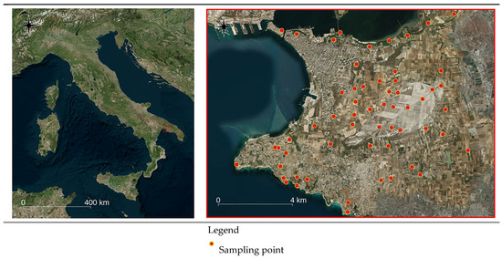
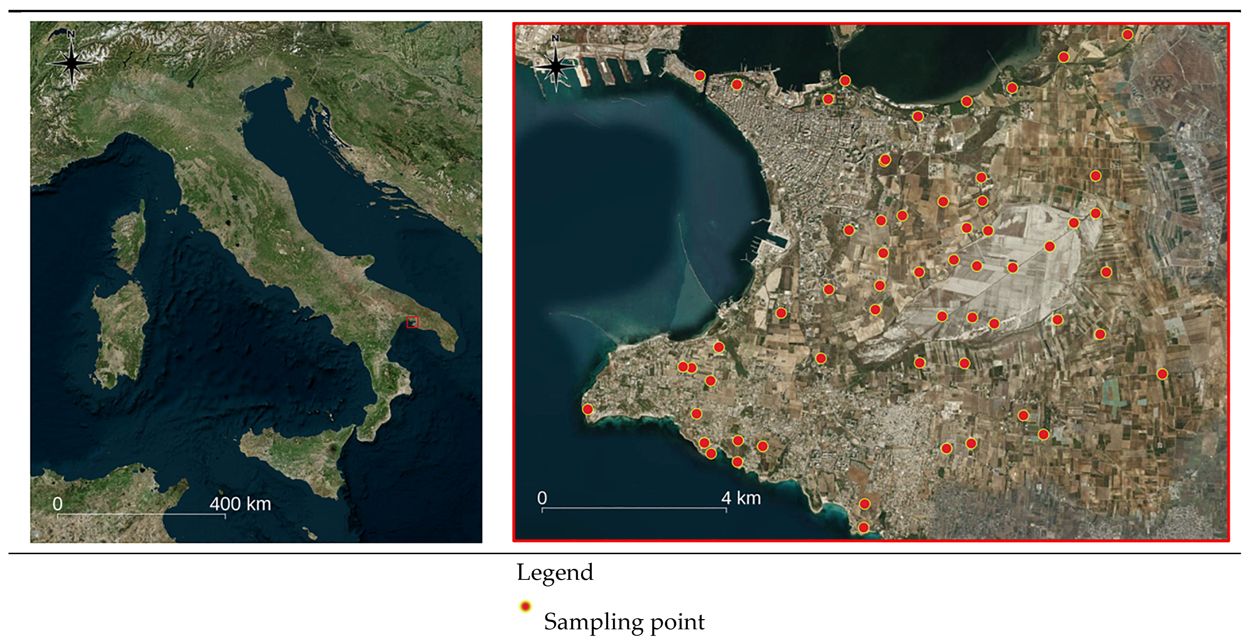
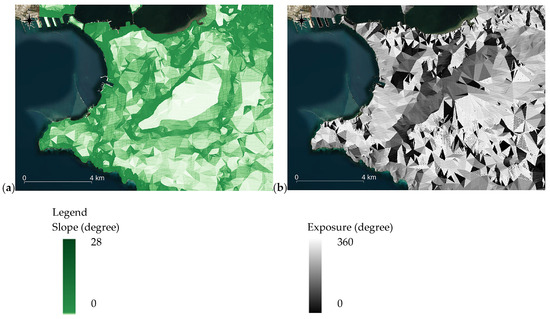
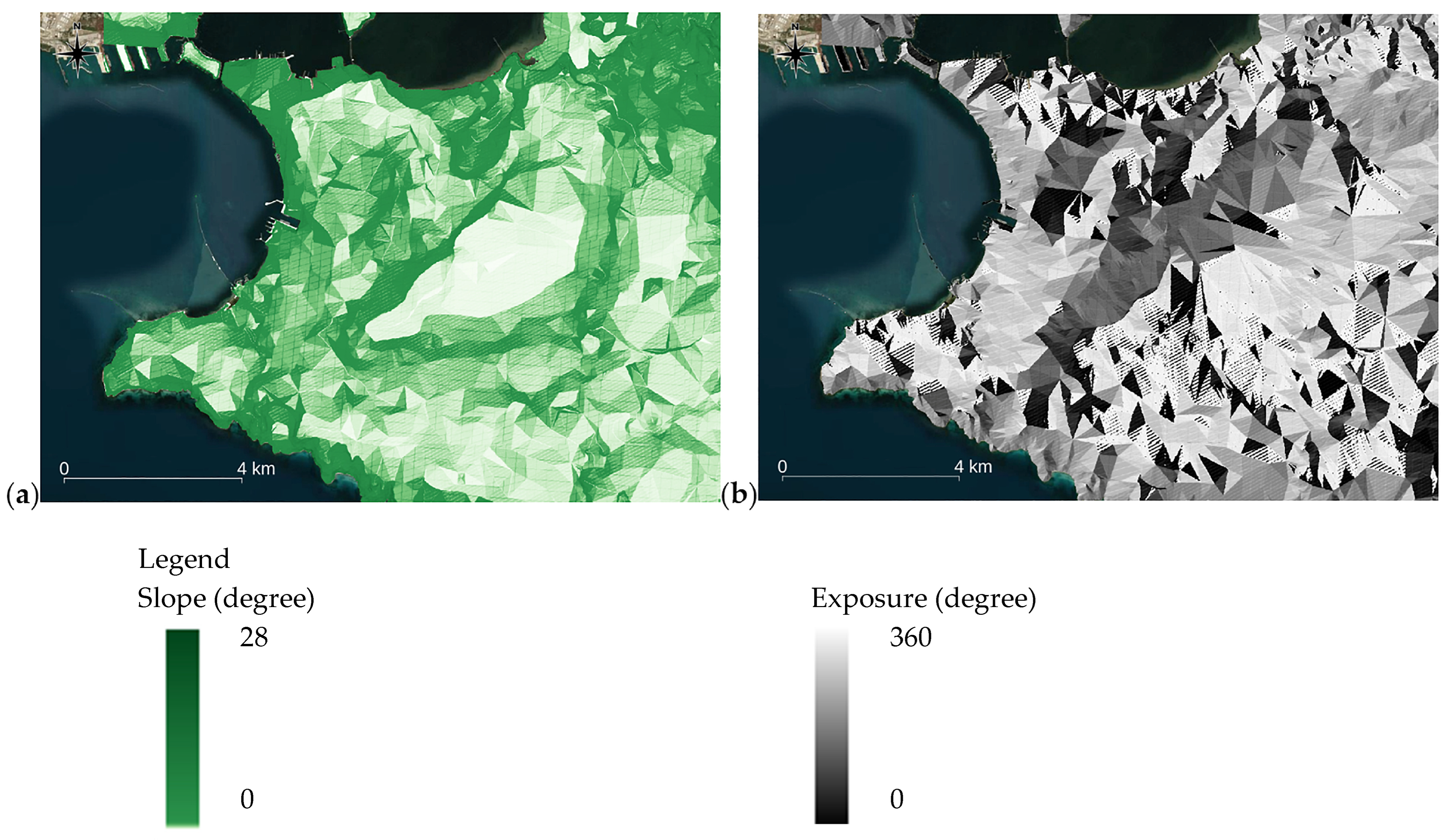
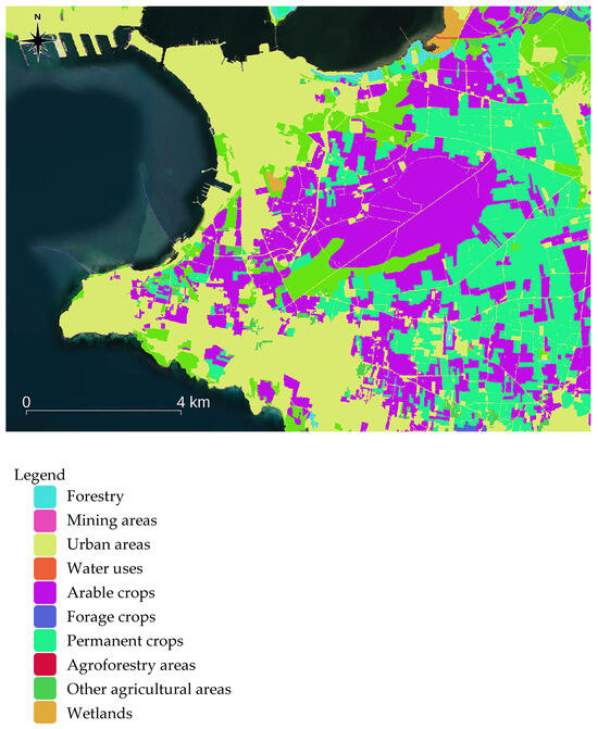
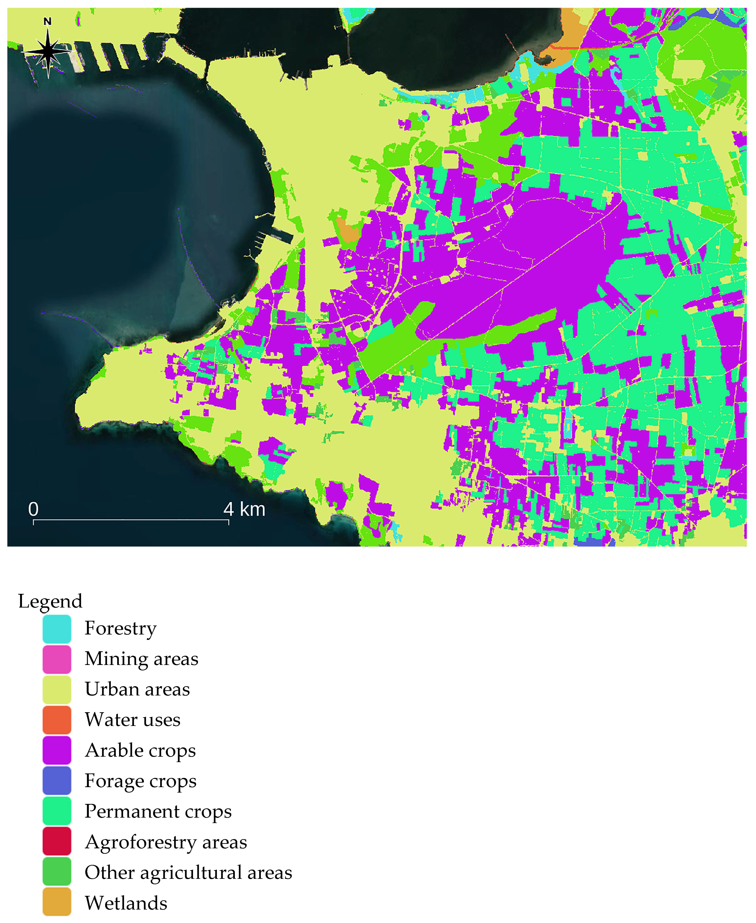
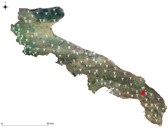
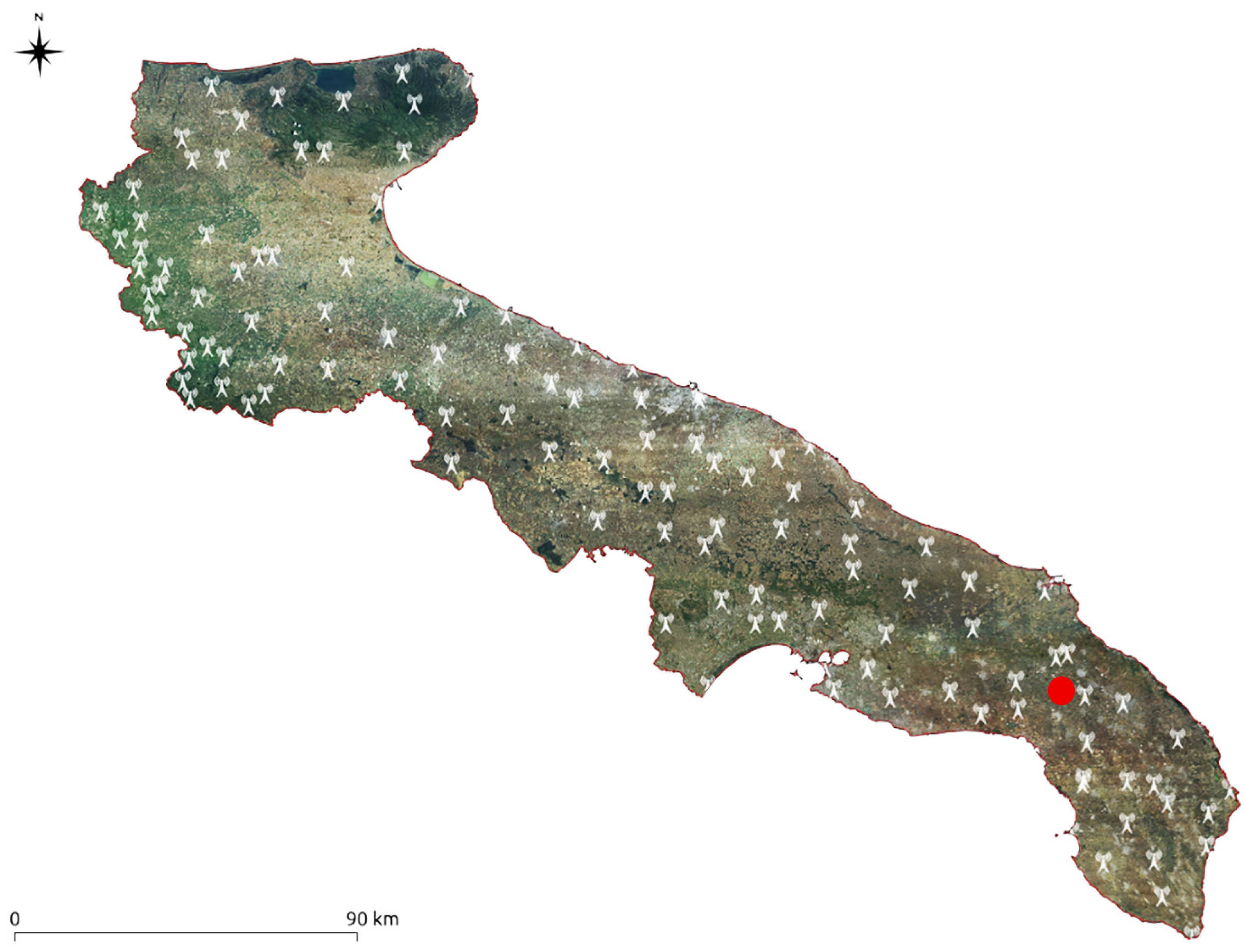
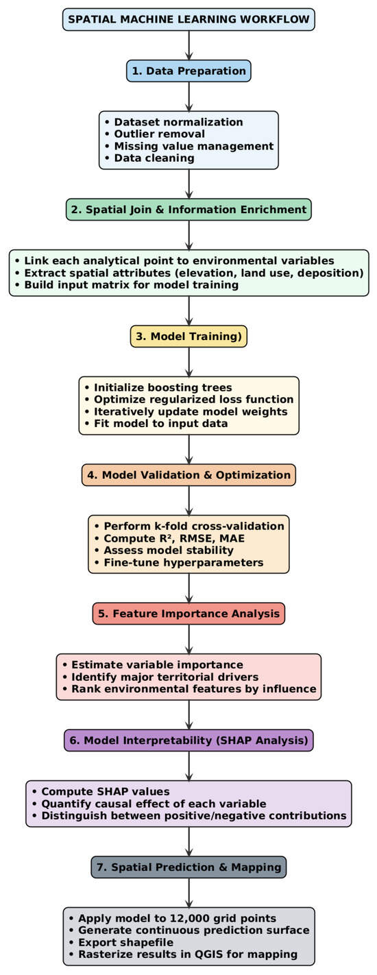
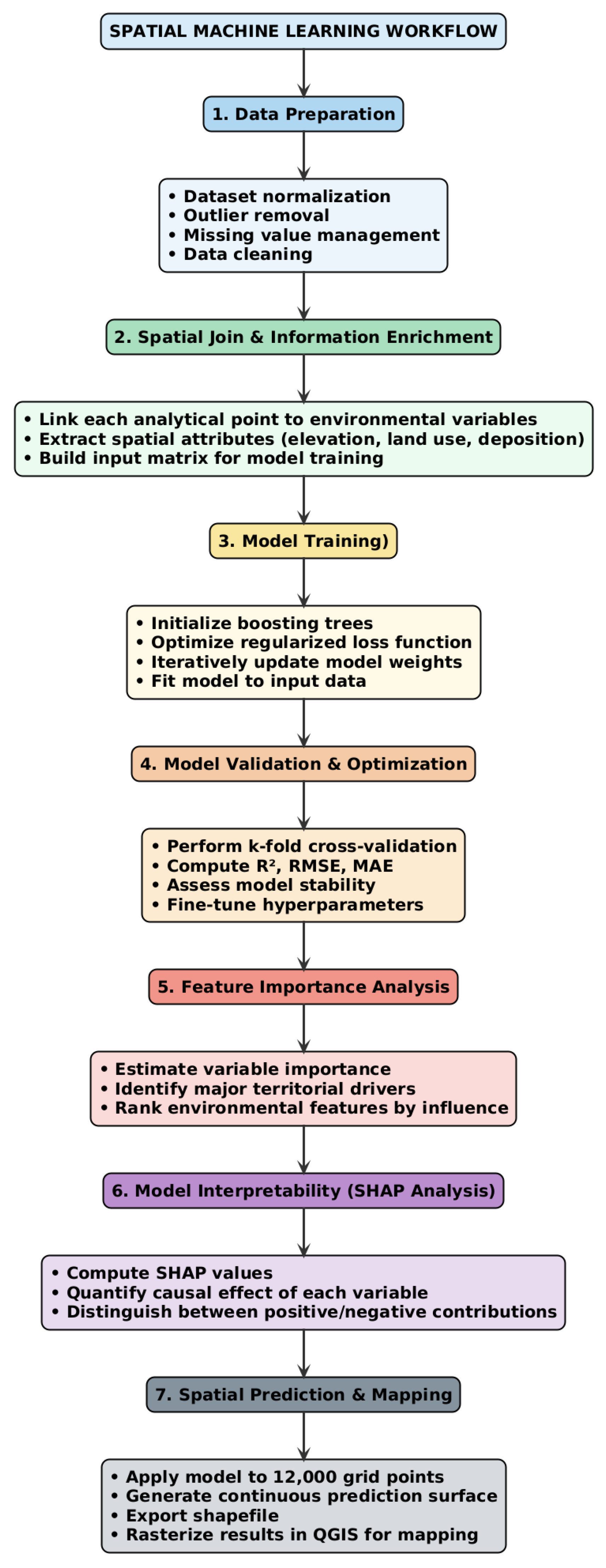
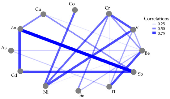
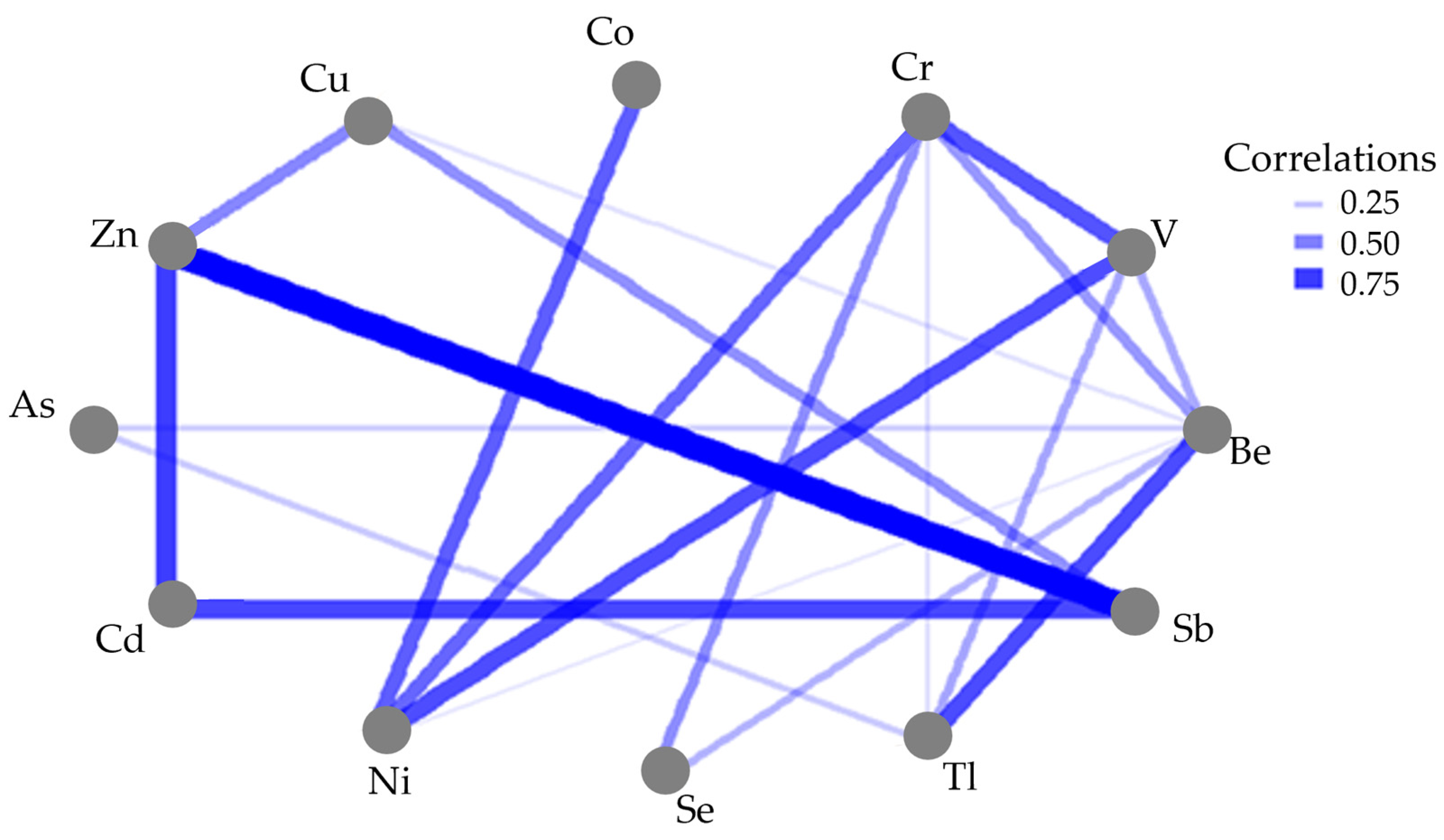
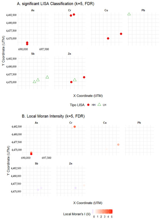
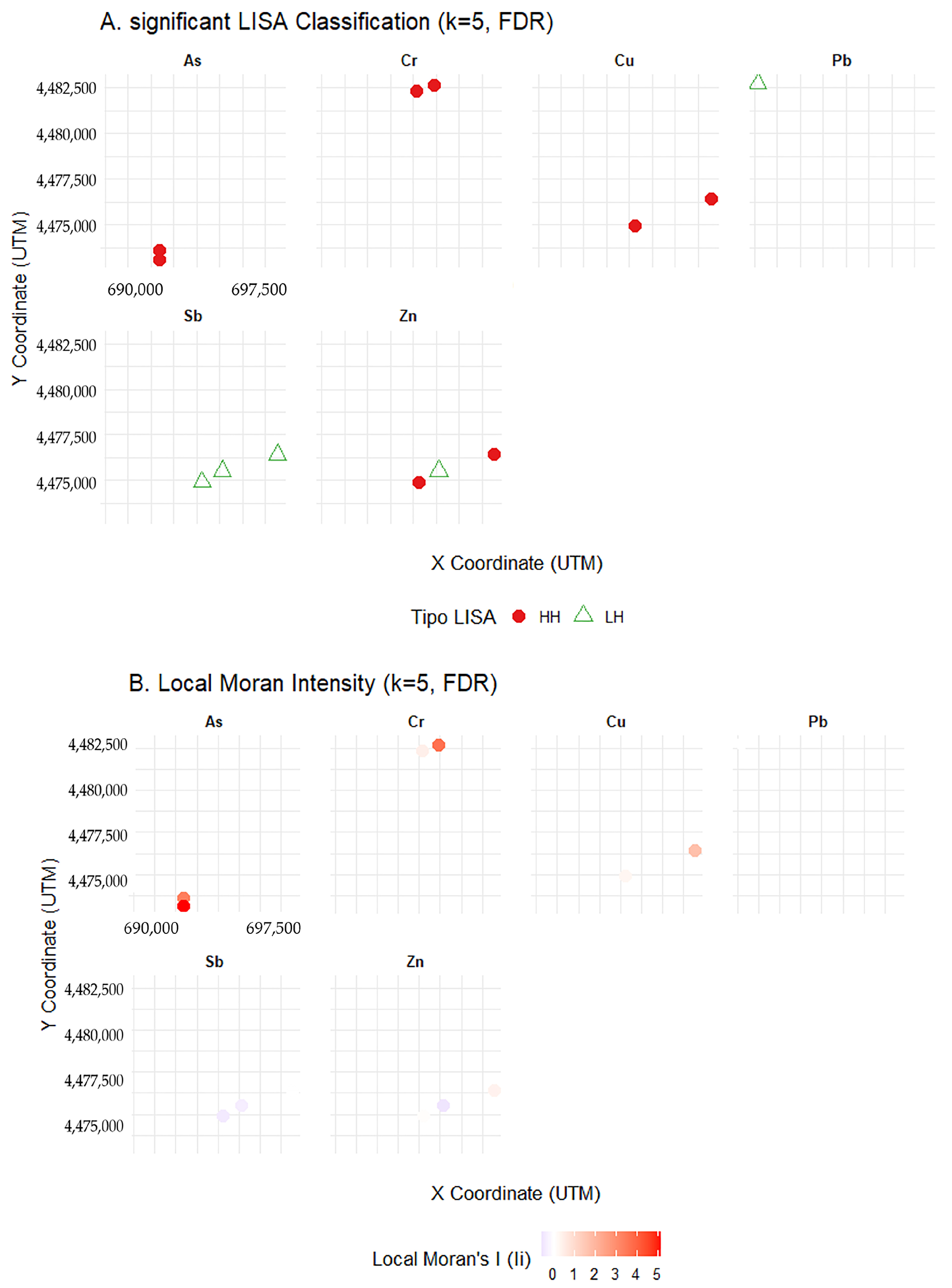
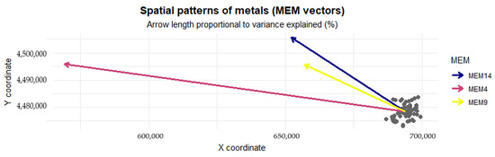
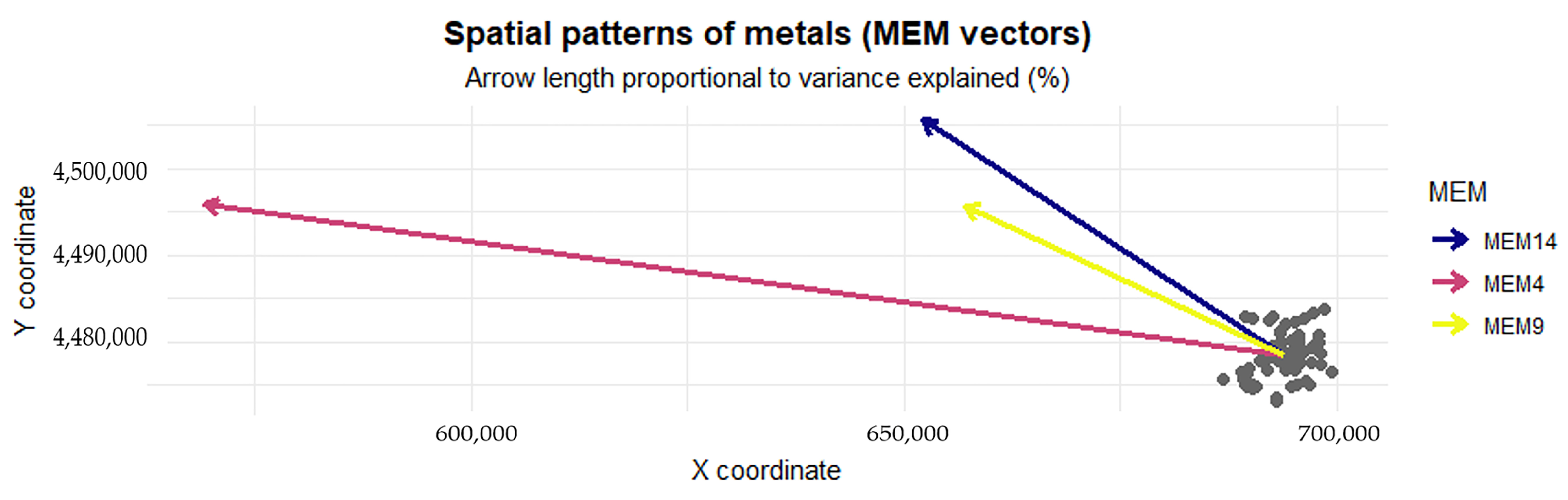
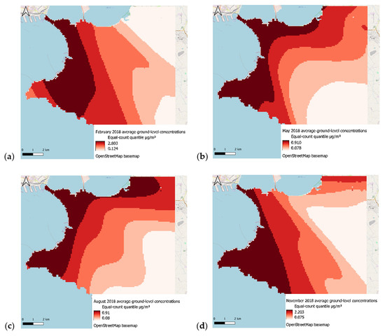
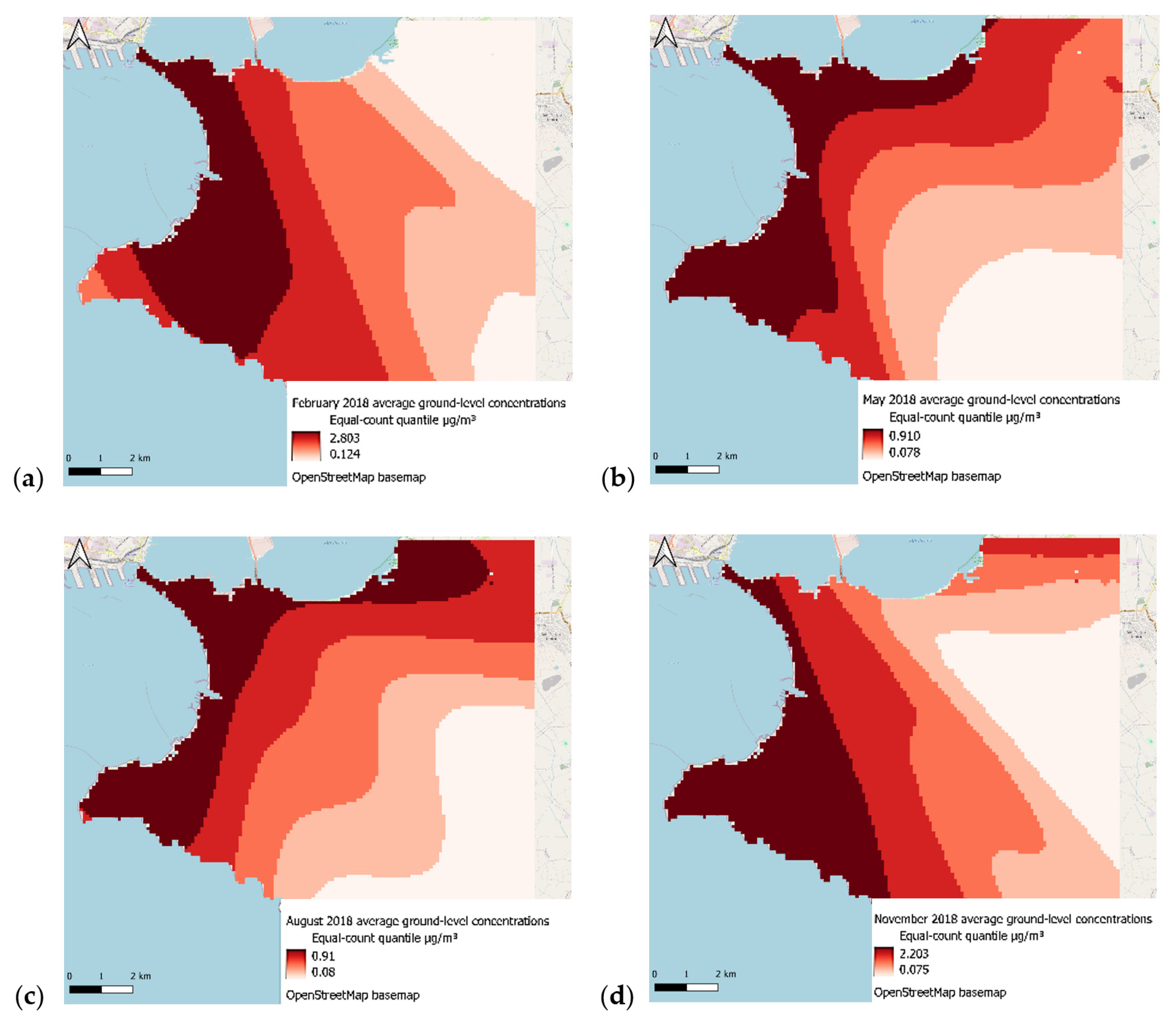
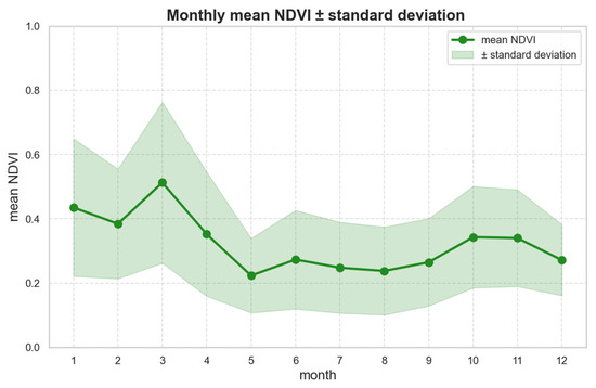
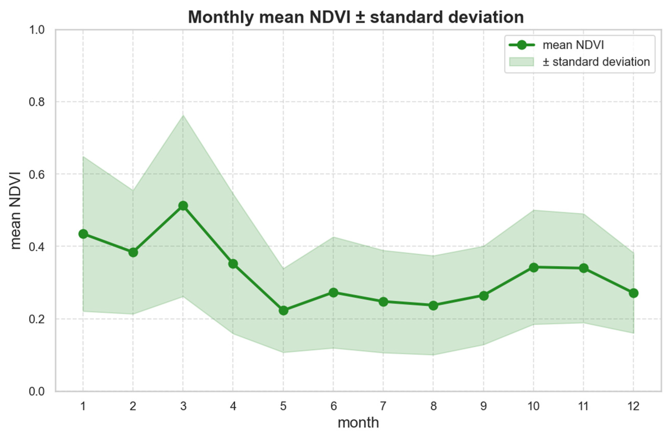
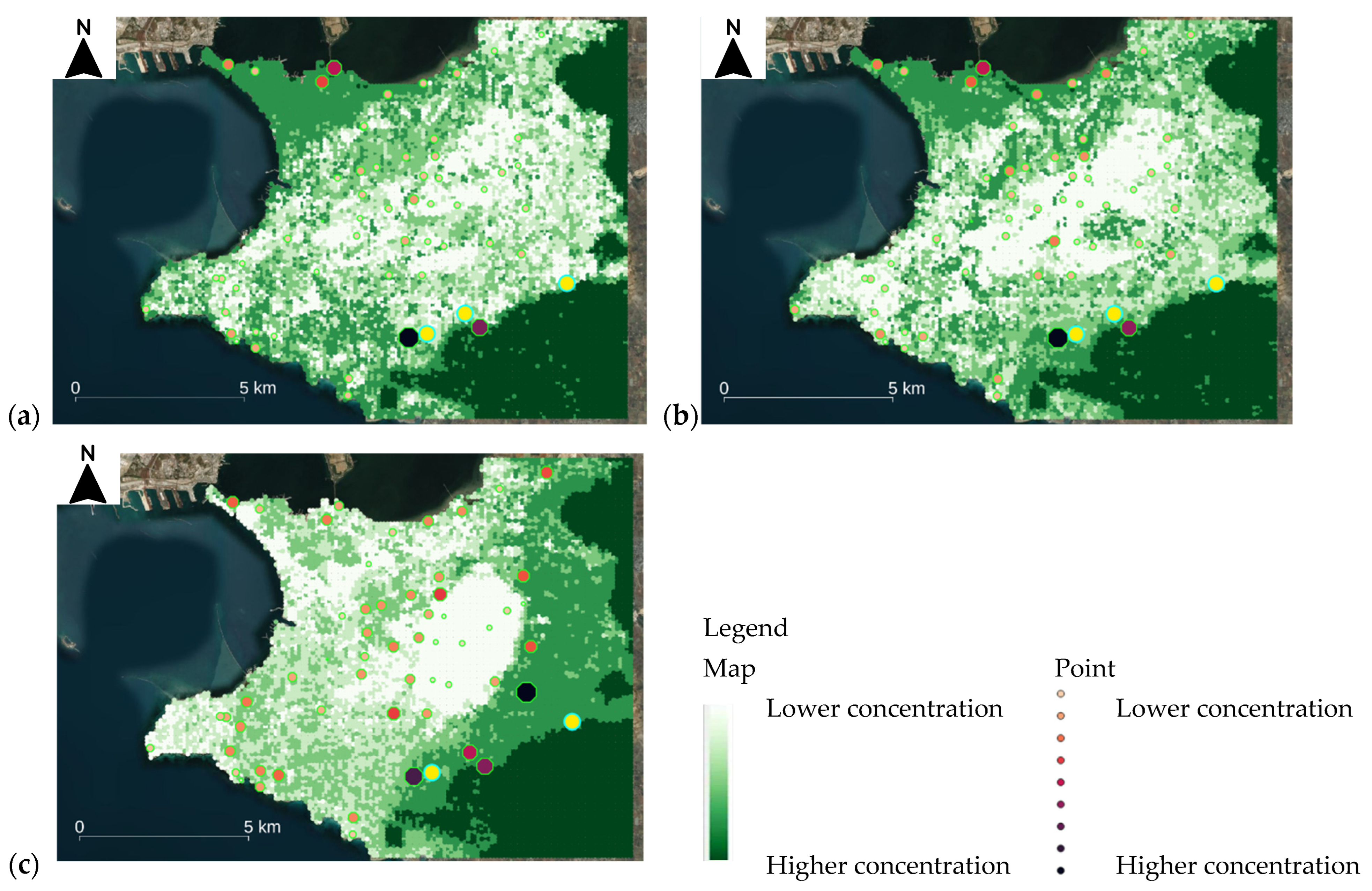

Disclaimer/Publisher’s Note: The statements, opinions and data contained in all publications are solely those of the individual author(s) and contributor(s) and not of MDPI and/or the editor(s). MDPI and/or the editor(s) disclaim responsibility for any injury to people or property resulting from any ideas, methods, instructions or products referred to in the content. |
© 2025 by the authors. Licensee MDPI, Basel, Switzerland. This article is an open access article distributed under the terms and conditions of the Creative Commons Attribution (CC BY) license.