Article

Sensitivity of WRF Operational Forecasting to AIFS Initialisation: A Case Study on the Implications for Air Pollutant Dispersion

by
Raúl Arasa Agudo
1,*,
Matilde García-Valdecasas Ojeda
2,3,
Miquel Picanyol Sadurní
4 and
Bernat Codina Sánchez
1,5
1
Applied Research Department, Meteosim, 08028 Barcelona, Spain
2
Applied Physics Department, University of Granada, 18071 Granada, Spain
3
Interuniversity Institute for Earth System Research in Andalusia (IISTA-CEAMA), 18006 Granada, Spain
4
Software Engineering Department, Meteosim, 08028 Barcelona, Spain
5
Applied Physics Department, University of Barcelona, 08028 Barcelona, Spain
*
Author to whom correspondence should be addressed.
Earth 2025, 6(4), 132; https://doi.org/10.3390/earth6040132
Submission received: 4 September 2025 / Revised: 3 October 2025 / Accepted: 16 October 2025 / Published: 17 October 2025
(This article belongs to the Section AI and Big Data in Earth Science)

Abstract

The Artificial Intelligence Forecasting System (AIFS), recently released by the European Centre for Medium-Range Weather Forecasts (ECMWF), represents a paradigm shift in global weather prediction by replacing traditional physically based methods with machine learning-based approaches. This study examines the sensitivity of the Weather Research and Forecasting (WRF) model to differentiate initial and boundary conditions, comparing the new AIFS with two well-established global models: IFS and GFS. The analysis focuses on the implications for air quality applications, particularly the influence of each global model on key meteorological variables involved in pollutant dispersion modelling. While overall forecast accuracy is comparable across models, some differences emerge in the spatial pattern of the wind field and vertical profiles of temperature and wind speed, which can lead to divergent interpretations in source attribution and dispersion pathways.

1. Introduction

Atmospheric pollution is one of the main problems of modern society [1]. On October 2024, the European Union approved a new air quality regulation, the European Directive 2024/2881/EC [2], that includes new pollutants, less permissive limits, and more restrictive actions to improve the air quality that citizens breathe. The Directive 2024/2881/EC increases the use of air quality modelling to manage the air quality, to take decisions, and to inform the public as soon as possible when the modelling applications show that thresholds will be exceeded. This air quality is not only determined by the emissions injected into the atmosphere, but also by the atmospheric conditions [3]. Thus, one of the key elements of any air quality forecasting system is weather forecasts.
Typically, the meteorological forecasts are generated using models that solve the equations governing atmospheric dynamics. These models are generally classified as either global or limited-area models [4]. Global models simulate atmospheric conditions across large regions or the entire planet, while limited-area models focus on specific geographical areas. Among the most widely used global models are the Global Forecasting System (GFS) [5], and the Integrated Forecasting System (IFS) [6]. As for limited-area models, the Weather Research and Forecasting (WRF) model [7] and the Harmonie-Arome model [8] are two of the most used worldwide. These models are run by national or regional weather administrations and by research centres and private companies that provide forecasting services to third parties.
Limited-area models (LAMs), also referred to as regional or mesoscale models, rely on global models to provide initial and lateral and boundary conditions (LBCs). Typically, data from global models is openly available to the user community.
During the last years, a new kind of modelling tool has appeared, and data-driven models have been applied for weather [9,10] and air quality forecasts [11,12]. These models usually are trained using numerical models and consider a high amount of measured data and remote sensing information in the case of weather application, and, moreover, traffic data and socio-economic parameters in the case of air quality applications.
Recently, as of 25 February 2025 (https://confluence.ecmwf.int/display/fcst/implementation+oF+Aifs+Single+v1 (accessed on 27 May 2025)), the European Centre for Medium-Range Weather Forecasts (ECMWF) has introduced a new model output alongside its traditional forecasts produced by the global IFS model. This addition includes predictions from its new artificial intelligence-based model AIFS (Artificial/Integrated Forecasting System) [13,14], specifically the AIFS Single V1 version.
AIFS was trained from processed data of the ECMWF Reanalysis v5 (ERA5) [15], covering the period between 1979 and 2022, as well as IFS forecasts from 2016 to 2022 [16]. Preliminary results show that AIFS improves the prediction of several meteorological variables across different regions of the globe [17]. Nevertheless, some limitations have been identified, such as reduced accuracy in representing high-resolution topographic effects, underestimation of wind speeds in tropical and extra-tropical cyclones, and occasional predictions of implausible precipitations in certain areas [16]. Limitations of state-of-the-art AI models in forecasting weather extremes have been identified recently [18].
Many studies analyse the performance evaluation of using GFS and IFS into mesoscale models [19] as boundary and initial conditions. In addition, benefits and limitations of data-driven models like AIFS have been identified recently [18,20]. But, given the novelty of AIFS, there is currently no published evidence of their application and impact as initial conditions and lateral boundary conditions (LBCs) for mesoscale models and how the use of AIFS into mesoscale or limited-area models can improve, or not, the meteorological information that is used for modelling dispersion purposes. Previous studies that confirm that the forecast of variables as precipitation or temperature using data-driven models [21] is better, or competitive at minimum, than using traditional numerical models, do not ensure to improve the forecast of relevant variables for air dispersion like wind fields or PBLH.
This research aims to evaluate how the use of AIFS predictions influences mesoscale forecasts generated by the WRF model, in comparison with those obtained using GFS and IFS outputs as initial and (LBC). In this study, particular attention is given to the sensitivity of meteorological parameters relevant to air quality applications, such as wind speed, wind direction, and planetary boundary layer height (PBLH). The study also examines differences in the calculation of backward trajectories, a common method for identifying potential emission sources responsible for odour events and/or exceedances of air quality limit values [22]. Additionally, the same comparative analysis is conducted using a dispersion model and an index that assesses conditions favourable to pollutant dispersion. A region of special interest from an air quality perspective has been selected as the study area.
Descriptions of the study area, the datasets employed, and methodology used to compare observed and modelled values are presented in Section 2. Section 3 presents the results of the analysis, followed by a discussion in Section 4. Finally, the main conclusions are summarised in Section 5.

2. Materials and Methods

This section outlines the episodes and datasets used in the analysis, describes the main geographical and environmental features of the Huelva region (the area of interest) and details the modelling approach adopted. It is structured in three subsections: area characteristics (Section 2.1), modelling approach (Section 2.2), and datasets, modelling period, and model evaluation (Section 2.3).

2.1. Area Characteristics

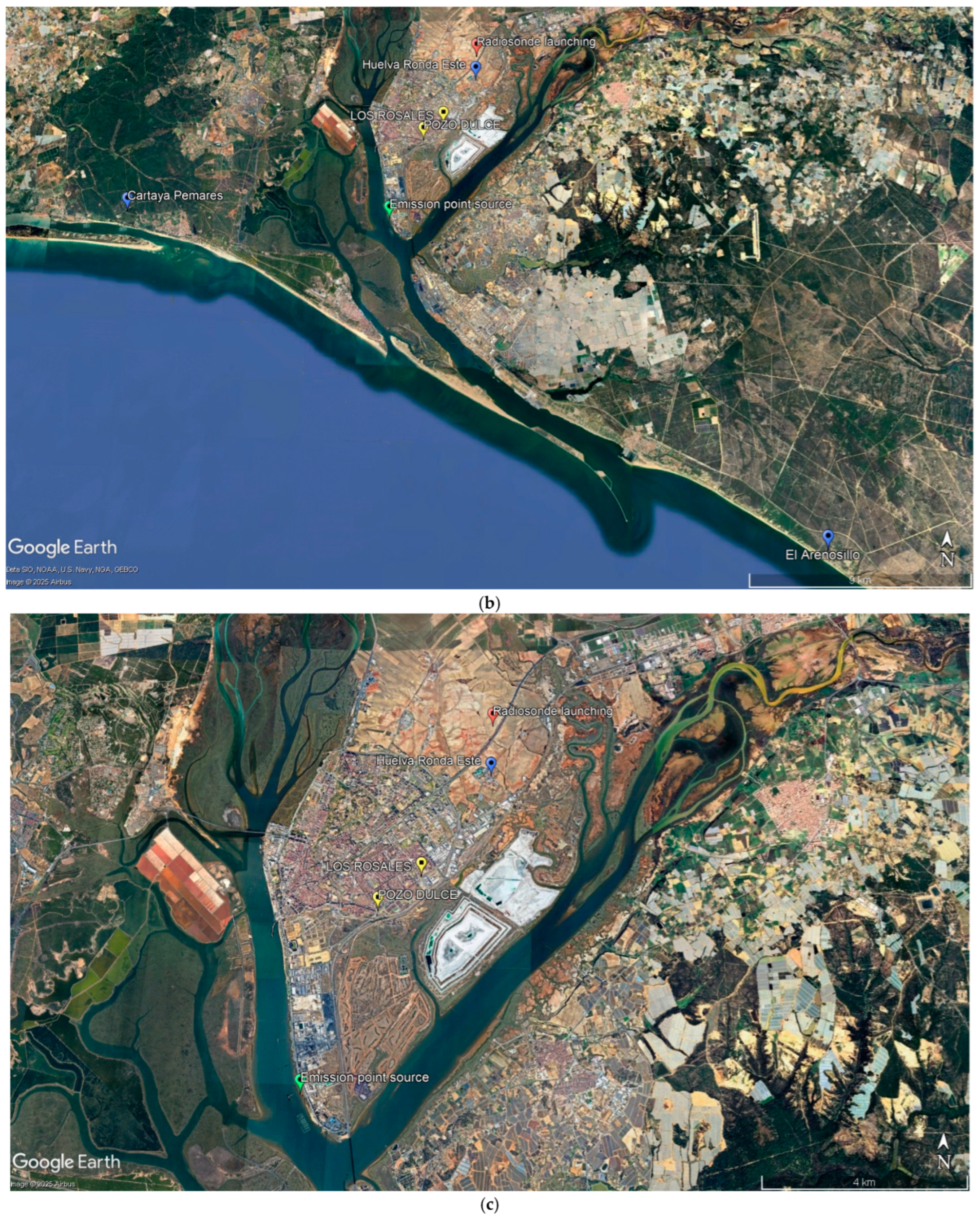
Huelva, located in southwestern Spain along the Gulf of Cádiz, sits at the confluence of the Odiel and Tinto Rivers and has a population of nearly 145,000 inhabitants (Figure 1). The region experiences a Subtropical-Mediterranean climate with Atlantic influence, characterised by hot, dry summers and mild, wet winters. Summer temperatures may exceed 40 °C, and the highest wind speeds typically occur at sunset. Severe gales (Beaufort scale force 9) occasionally affect the area throughout the year.
The city of Huelva and its metropolitan area encompass the main population centre of the province, alongside greenhouse zones, protected natural areas (including proximity to Doñana National Park), and one of the most significant industrial hubs in southern Spain. As such, Huelva represents a complex urban environment influenced by industrial emissions [23]. Air quality and source contributions, both natural and anthropogenic, have been extensively studied in the region over the past decades [24,25,26,27,28,29,30,31,32].

2.2. Modelling Approach

2.2.1. WRF Modelling System

The regional and mesoscale meteorological model used in this study is the Weather Research and Forecasting-Advanced Research model (WRF-ARW) [7], version 4.3.3, developed by the National Center of Atmospheric Research (NCAR). WRF is a next-generation numerical system widely used for both operational forecasting and regional climate research [33,34,35,36,37,38,39]. It is a fully compressible, non-hydrostatic model, with a terrain-following hydrostatic pressure coordinate. WRF offers a broad range of parameterisations, which are simplified representations of physical processes occurring at scales smaller than the model’s resolution, which are essential for ensuring model accuracy across varying climatic and geographic conditions. The choice of parameterisation schemes is therefore critical to improving forecast reliability [40,41,42,43,44].
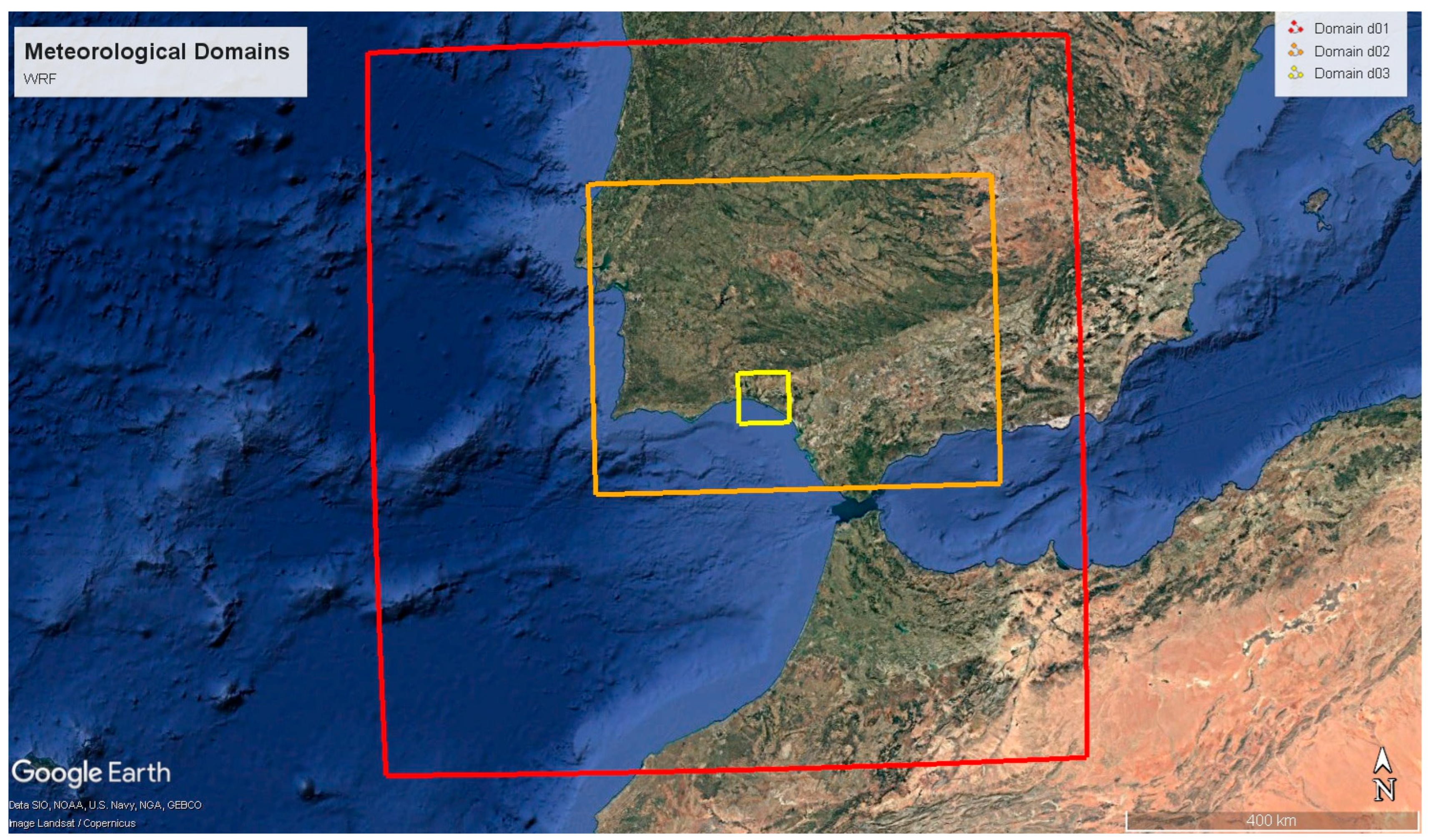
The modelling domains used in this study are shown in Figure 2. The parent domain (d01), with a grid point spacing of 9 km and aimed to capture synoptic features and general circulation patterns, is centred at 37.14° N, 7.38° W and encompasses the southwestern Iberian Peninsula, northern Morocco, and adjacent marine areas. It spans approximately 900 × 909 km2 (west–east × south–north). The first nested domain (d02), at 3 km resolution, covers southern Portugal and western Andalusia (507 × 390 km2), while the innermost domain (d03), with a grid point spacing of 1 km, focuses on the Huelva region (64 × 64 km2). Domain configuration follows the approach described in [42].
For this study, the WRF model was configured for operational forecasting using the parameterisation schemes proposed by [42] and summarised in Table 1. These schemes were selected based on their demonstrated ability to accurately simulate wind speed, wind direction, temperature, and relative humidity. Parameterisations were kept fixed throughout the simulations, as the objective was to assess the sensitivity of forecasts to different initialisations and LBCs from global models, rather than to evaluate the impact of varying physical schemes.
A total of 42 vertical levels were defined, with 25 levels below 1500 m above ground level (a.g.l.), and the lowest level positioned at approximately 8 m a.g.l. Vertical resolution was increased near the surface to enhance the accuracy of wind-related variables, as supported by previous studies [42,45].
Topography and land use data were selected from the default WRF databases, using the highest available resolution: GTOPO30 for elevation and USGS categories for land use, both at 30 arc-seconds (~1 km at the equator). Although higher-resolution datasets could potentially improve forecast performance [42,46], they were not employed in this study to maintain focus on the effects of different initialisations and LBCs.
Table 1. Configuration options selected in WRF.
Scheme/Parameterisation/OptionOption Selected
Modelling Domainsd01, d02, d03
Horizontal resolution9 km (d01), 3 km (d02), 1 km (d03)
Vertical levels42, 25 below 1500 m a.g.l
Lowest level8 m a.g.l
TopographyGTOPO30
Land UsesUSGS
MicrophysicsSBU-Lin [47]
Longwave RadiationRRTMG [48]
Shortwave RadiationDudhia [49]
CumulusKain-Fritsch [50]
Surface LayerMM5 similarity [51]
Land SurfaceNoah LSM [52]
Planetary Boundary LayerYonsei University [53]
A total of 30 simulations were conducted, each spanning 78 h. The first 6 h were treated as a spin-up period to reduce the impact of initial conditions.

2.2.2. Global Model Initialisations

Three different global models were used to provide initial conditions and LBCs for the WRF mesoscale simulations: GFS, IFS, and AIFS.
GFS is provided by the National Centers for Environmental Prediction (NCEP, https://www.nco.ncep.noaa.gov/pmb/products/gfs/ (accessed on 27 May 2025)) with a horizontal resolution of 0.25°, and it is updated every 6 h (00, 06, 12 and 18 UTC).
IFS and AIFS are supplied by ECWMF (https://data.ecmwf.int/ (accessed on 27 May 2025)) also with a spatial resolution of 0.25°. IFS is updated every 12 h (00 and 12 UTC), and AIFS every 6 h (00, 06, 12 and 18 UTC).
The forecast horizons are 384 h for GFS, and 360 h for both IFS and AIFS. GFS provides 41 vertical levels, whereas IFS and AIFS offer 13 levels. In all three models, the first vertical level is located at 1000 hPa. The second level is near the surface: at 975 hPa for GFS, and at 925 hPa for IFS and AIFS. The highest vertical level reaches 0.01 hPa in GFS and 50 hPa in IFS and AIFS.
Regarding temporal resolution, GFS provides hourly data for the first 120 forecast hours, and 3-hourly data from 120 to 384 h. IFS offers 3-hourly data up to 144 h, and 6-hourly data from 144 to 360 h. AIFS provides 6-hourly data throughout the entire forecast period.
These specifications refer to publicly available open-data products suitable for initializing mesoscale models. In all cases, simulations were initialised using global model outputs corresponding to 00 UTC.

2.2.3. Transport and Dispersion Modelling

The HYSPLIT transport and dispersion model [54] was used to assess potential changes in the forecast of backward trajectories resulting from different initialisations. This analysis focused on specific pollutant episodes.
Backward trajectories were computed using both the “normal” and “ensemble” options in HYSPLIT, starting at a height of 1.5 m above ground level (m.a.g.l.). The selected episodes were defined based on data from air quality monitoring stations, considering the maximum 10 min SO2 concentrations during the study period. SO2 was chosen as the target pollutant due to its relevance in the region [55].
Backward trajectory analysis was complemented with dispersion modelling. The aim of the modelling dispersion analysis is to analyse how the use of GFS/IFS/AIFS affects the HYSPLIT forecasts using an illustrative emission. For this purpose, a hypothetical point emission source was defined at coordinates 37.22° N and 6.95° W (Figure 1), located at 10 m.a.g.l., with an emission rate of 40 g/s for one hour starting at 14:00 UTC. SO2 was, again, used as the tracer pollutant. This setup does not correspond to a real emission event; its sole purpose was to evaluate the sensitivity of dispersion modelling to the different WRF meteorological configurations. The point emission source is located in the industrialised area of Huelva [56].

2.2.4. Ventilation Index

The ventilation index (VI) is defined as the product of wind speed and planetary boundary layer height (PBLH). This index is widely used in various regions to regulate outdoor burning and to support air quality management decisions [57,58].
In this study, we adopted the classification proposed by [59], which categorises VI as follows: poor: 0–1175 m2/s; marginal: 1176–2350 m2/s, fair: 2351–3525 m2/s; good: >3525 m2/s.
This classification was used to compare the different WRF configurations considered. For the VI calculation, wind speed at 10 m above ground level (m.a.g.l.) was used.

2.3. Datasets, Modelling Analysis Period and Model Evaluation

2.3.1. Meteorological and Air Quality Station Data

Local meteorological stations managed by the Spanish National Meteorological Agency (AEMET) were used to evaluate the performance of the different simulations. The selected stations include Huelva Ronda Este (37.28° N, 6.91° W, 19 m.a.s.l), Cartaya Pemares (37.22° N, 7.08° W, 15 m.a.s.l), and El Arenosillo (37.10° N, 6.74° W, 41 m.a.s.l). Their geographical locations are shown in Figure 1. Wind direction data from AEMET is provided in 45-degree intervals, allowing us to only distinguish winds from N, NE, E, SE, S, SW, W, and NW.
To select episodes for transport modelling, data from local air quality stations were considered. These stations belong to the Surveillance and Control of the Atmospheric Pollution network, managed by the Andalusian Government [60]. Their locations are also shown in Figure 1. The selected air quality stations are Los Rosales (37.26° N, 6.93° W, 6 m.a.s.l.) and Pozo Dulce (37.25° N, 6.94° W, 14 m.a.s.l.).
Both stations are located in the city of Huelva and were chosen due to their relevance in capturing industrial emissions in the region [55].

2.3.2. Modelling Analysis Period

Simulations were conducted over the period from 6 April to 5 May, 2025. This timeframe was selected due to different reasons. On one hand, this period contains notable meteorological variability, allowing the results to be representative of a range of atmospheric conditions; secondly, because the SO2, that is the pollutant selected, usually does not achieve very high or very low levels in this period in Huelva [55]; and finally, because two months ago (at the end of February), the version of AIFS considered in this analysis was launched.
Between 6 and 13 April, Huelva was affected by Storm Olivier [61], followed by the arrival of several Atlantic fronts, which brought multiple rainfall episodes. The most significant occurrence was on 14 April, with 6 mm of accumulated precipitation over 24 h. In the subsequent days, weather conditions were dominated by the Azores Anticyclone and North African air masses, resulting in stable atmospheric conditions and maximum temperatures reaching 29 °C on 24 April. During the final week of the study period (27 April to 5 May), additional Atlantic fronts entered the region, causing a slight drop in temperature and sporadic rainfall, with the most notable event being 17 mm recorded on 30 April.
According to [62], April 2025 in the province of Huelva was warmer and wetter than average, with a monthly mean temperature of 0.8 °C above climatological average and total precipitation of 71.6 mm, representing 138% of the climatological monthly average.
SO2 has been selected as a pollutant to analyse in this study because it is one of the most relevant pollutants that affect the city of Huelva, and because other pollutants like NO2 or particulate matter can be affected, in general, by other relevant emissions like traffic or nature. To facilitate the analysis and because high levels of this pollutant were identified during the modelling period, SO2 was selected as tracer pollutant for this research.
From an air quality perspective, the selected period includes two notable episodes of elevated SO2 concentrations linked to industrial emissions in the city of Huelva. These episodes are illustrated in Figure 3. To minimise the influence of reduced planetary boundary layer height (PBLH), both episodes were selected during midday hours, when the PBLH typically reaches its diurnal maximum. This timing ensures that the observed SO2 levels are directly influenced by wind-driven transport of industrial emissions.
During Episode 1, a maximum 10 min SO2 concentration of 103 µg/m3 was recorded at Pozo Dulce station at 3:20 p.m. (local time, UTC + 2) on 24 April. In Episode 2, a peak concentration of 168 µg/m3 was measured at Los Rosales station at 3:50 p.m. on April 27. Both episodes were characterised by spring-like conditions with stable atmospheres, maximum temperatures of 29 °C (24 April) and 27 °C (27 April), and no precipitation. On April 24th, light winds dominated the city of Huelva, with velocities below 4 m/s, reaching a maximum wind gust of 7 m/s. Winds were easterly at the beginning of the day, and from 3:00 p.m. until the end of the day, southerly winds dominated, with SW winds being dominant between 3:00 p.m. and 6:00 p.m., hours when the highest SO2 values were measured. On 27 April, light winds dominated the city of Huelva, with velocities below 5 m/s, reaching a maximum wind gust of 9 m/s. Winds were from the east and north at the beginning of the day, and from 2 p.m. until the end of the day, the south component dominated, with the SW component being dominant between 2 p.m. and 5 p.m., hours that correspond to the highest SO2 values measured.

2.3.3. Radiosonde Data

To assess the sensitivity of the simulations with respect to vertical profiles within the planetary boundary layer (PBL), radiosonde data have been incorporated into the analysis. Specifically, upper-air meteorological measurements obtained from radiosonde launches conducted by AEMET (location indicated in Figure 1) were considered.
AEMET carries out automated radiosonde launches twice a day, at approximately 00 and 12 UTC (corresponding to local time UTC + 2 for the selected episodes). These measurements provide detailed information on key atmospheric variables, including temperature (°C), dew point (°C), relative humidity (%), wind speed (m s−1), wind direction (°), and atmospheric pressure (hPa), spanning from the surface up to an altitude of approximately 30 km [63].
The radiosonde data used in this study were retrieved from the METEOCIEL website (https://www.meteociel.fr/observations-meteo/sondage.php?map=1 (accessed on 27 May 2025)).

2.3.4. Forecast Evaluation and Forecast Sensitivity Analysis

To evaluate the forecast performance and sensitivity to different global initialisation models, a combined approach was adopted, integrating numerical deterministic evaluation with visual and graphical comparisons. The analysis focused on four key meteorological variables: wind speed, wind direction, temperature, and relative humidity.
To quantify forecast accuracy, four statistical metrics were selected from among the many available methodologies [64,65]: the Mean Bias (MB), the Mean Absolute Gross Error (MAGE), the Root Mean Square Error (RMSE), and the Index of Agreement (IOA). The IOA measures the degree of agreement between the deviations in predictions and observations from their respective means [42]. These metrics provide insight into model uncertainty relative to observations, and benchmarks were established following the recommendations in [66,67].
The analysis has been carried out over domain d03, the innermost modelling domain (Figure 2). Table 2 presents the statistical results for each meteorological parameter along with the corresponding benchmarks. For wind speed and direction, calms below 1 m s−1 were excluded from the analysis, as wind direction is unreliable under such conditions [44,68]. All statistics were computed using hourly data from both model outputs and observational records, and performance was assessed for 24 h, 48 h, and 72 h forecasts.
This numerical evaluation was complemented by several qualitative analyses:
  • A visual inspection of spatial differences. Bidimensional maps were generated to compare the geographical distribution of variables across WRF simulations initialised with different global models.
  • A comparison of diurnal cycles. Observed and simulated diurnal cycles were compared at meteorological stations within the modelling domain.
  • A comparison of wind roses. Observed wind roses were contrasted with those simulated by WRF, focusing on the station located in the city of Huelva.
  • A comparison of the vertical profiles. Simulated vertical profiles of key variables were compared against radiosonde measurements to assess consistency across different initialisations.
  • Impact on backward trajectories. Backward trajectories were analysed for real pollutant episodes to determine whether different initialisations led to divergent potential emission sources.
  • Impact on dispersion modelling. Simulations using SO2 as a tracer from a hypothetical point source were used to evaluate how meteorological inputs influence dispersion patterns, particularly in scenarios involving industrial emissions.
  • A comparison of the ventilation index (VI). VI values were calculated using different global model initialisations to assess their influence on atmospheric dispersion potential.

3. Results

The following sections present the main findings of the study: deterministic forecast evaluation, analysis of diurnal profiles and wind roses, visual inspection of spatial differences, comparison of vertical profiles, assessment of the impact of different global model initialisations in WRF on backward trajectories, evaluation of dispersion modelling sensitivity, and comparison of the ventilation index across configurations.

3.1. Numerical Evaluation

The statistical results derived from the metrics listed in Table 2 are summarised in Table 3. The evaluation covers the entire modelling period and includes data from the three available monitoring stations within the region. The analysis was conducted over the d03 modelling domain for three forecast horizons: 24, 48, and 72 h.

3.2. Diurnal Cycles

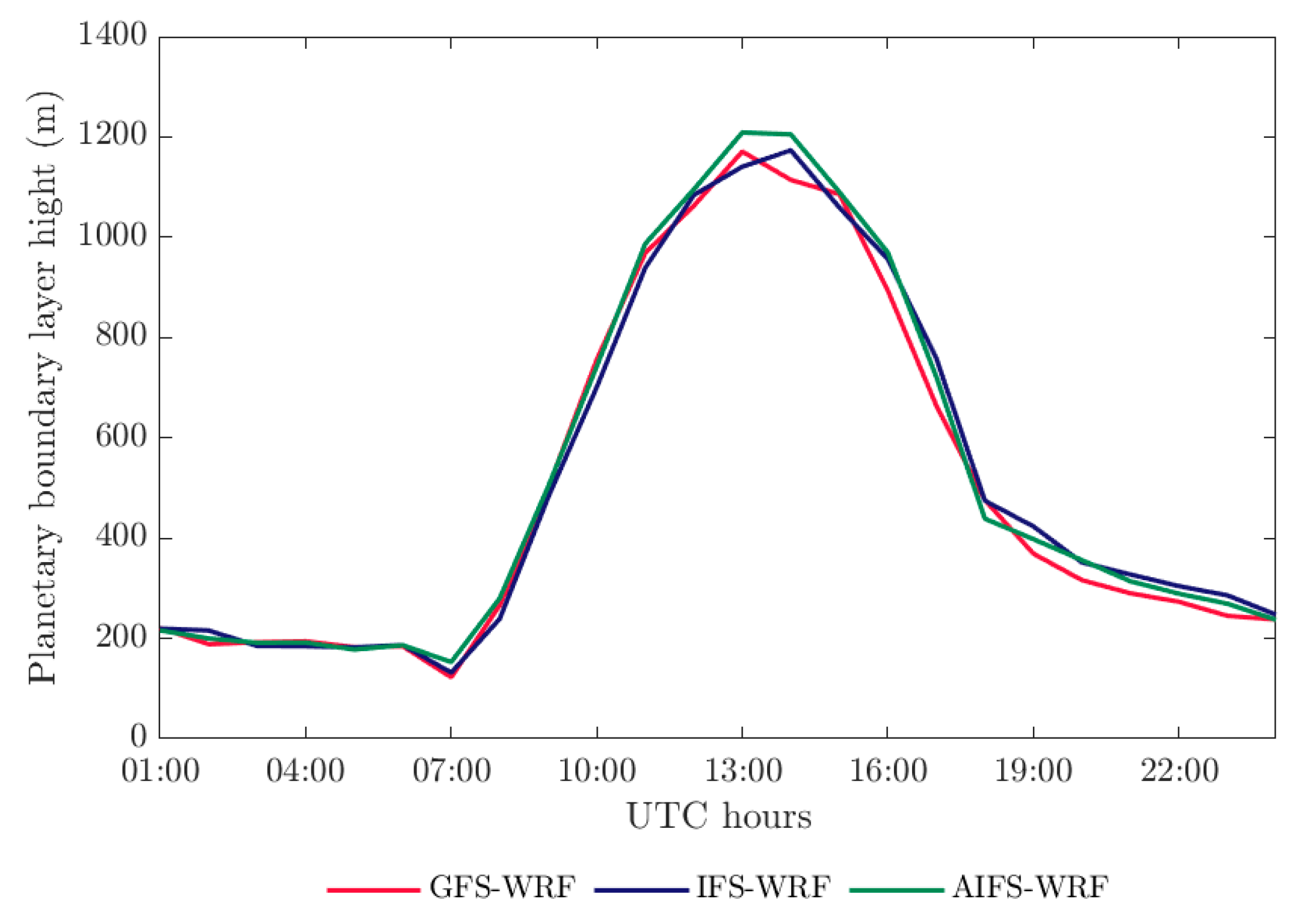
Figure 4 presents the diurnal cycles of temperature, wind speed, and relative humidity obtained from the different WRF simulations, alongside observed values recorded at official meteorological stations. The comparison is based on the average across the three forecast horizons: 24, 48, and 72 h. Figure 5 displays the estimated planetary boundary layer height (PBLH) for each WRF configuration, focusing on the Huelva Ronda Este station.

3.3. Wind Rose Analysis

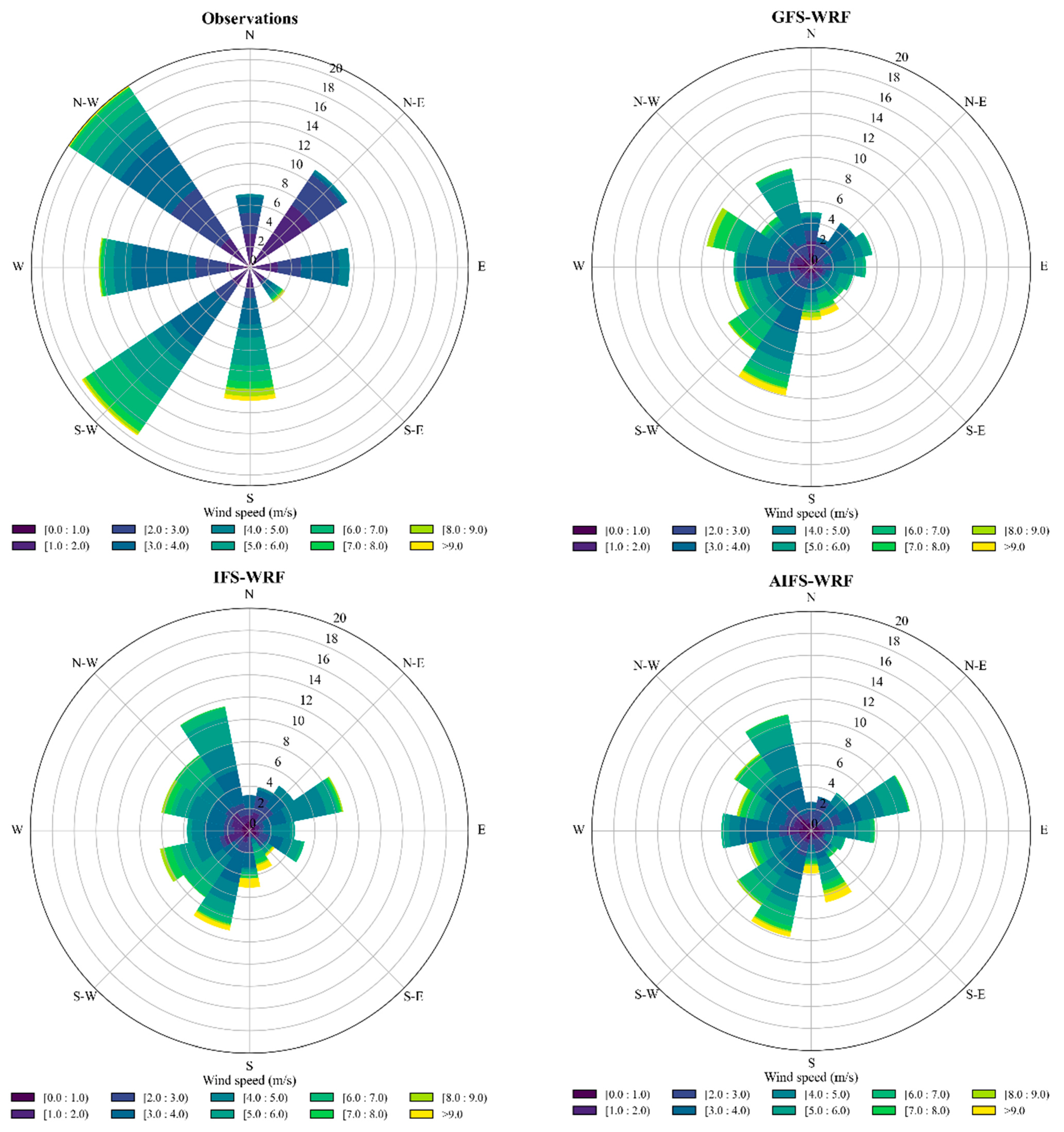
Figure 6 displays the wind roses derived from the various WRF simulations, alongside those corresponding to observed data at the official meteorological station of Huelva Ronda Este. This comparison allows for a visual assessment of the prevailing wind directions and frequencies reproduced by each model configuration.

3.4. Visual Inspection of Differences

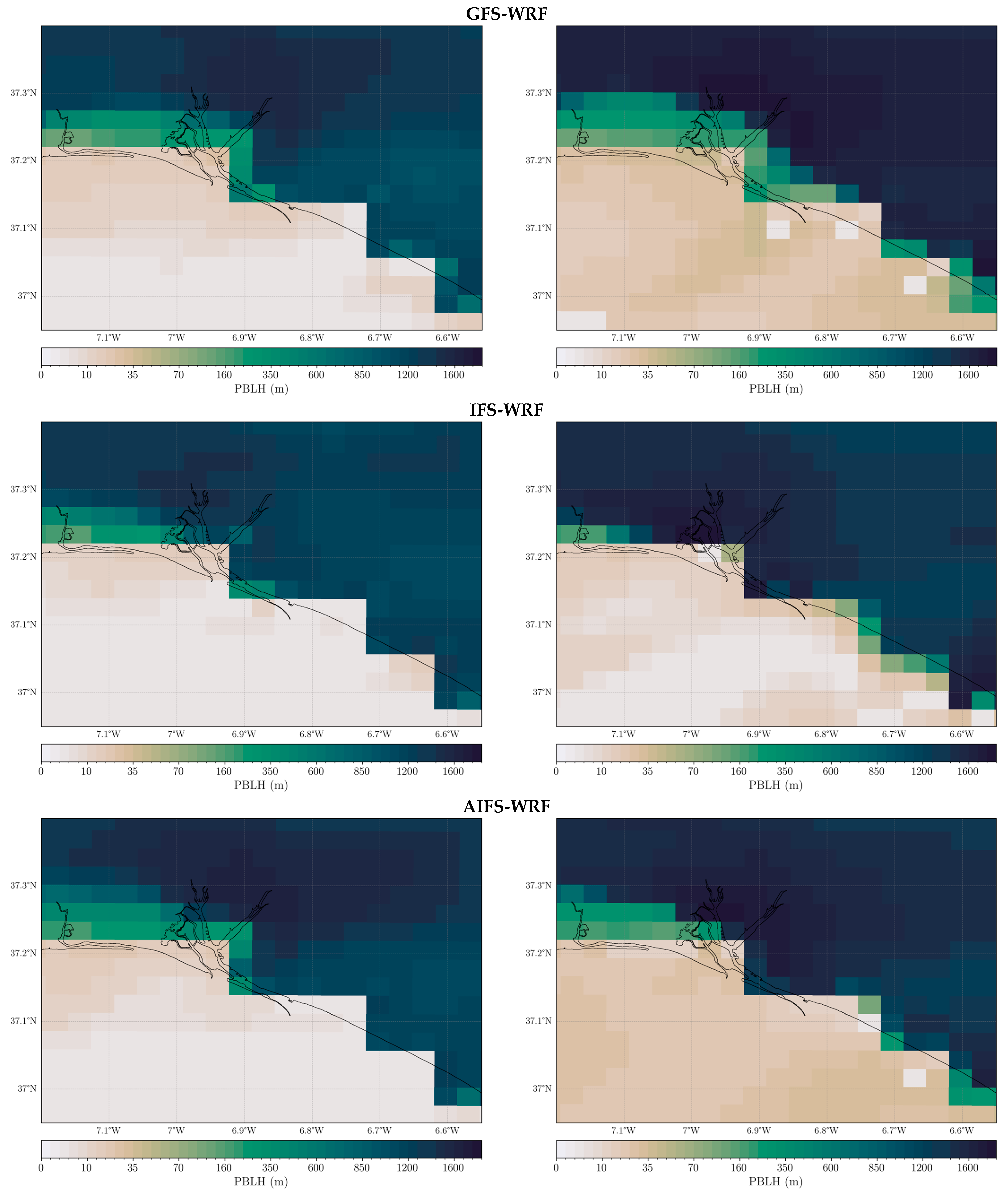
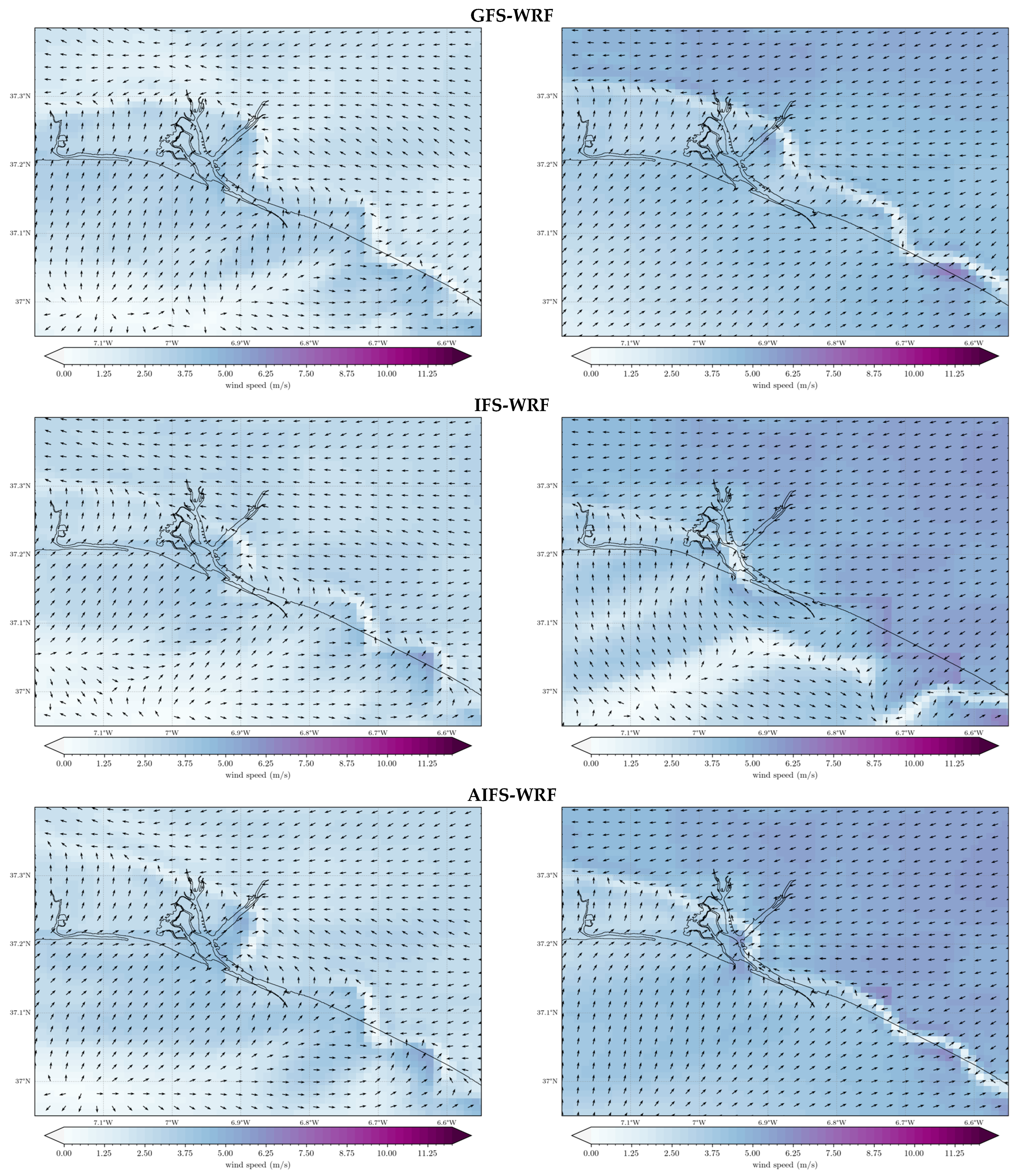
Figure 7 and Figure 8 present spatial maps of selected meteorological parameters for 24 April and 27 April, 2025. These dates were chosen as illustrative cases due to the elevated SO2 concentrations recorded and the presence of pronounced atmospheric stability, which limited pollutant dispersion across the study area.
The meteorological parameters analysed include planetary boundary layer height (PBLH), wind speed, and wind direction at 10 m above ground level, within the innermost modelling domain (d03).
In Figure 9, the wind field distribution and temporal evolution between 11 a.m. and 2 p.m. on 27 April 2025 are presented for each WRF simulation.

3.5. Comparison of Vertical Profiles

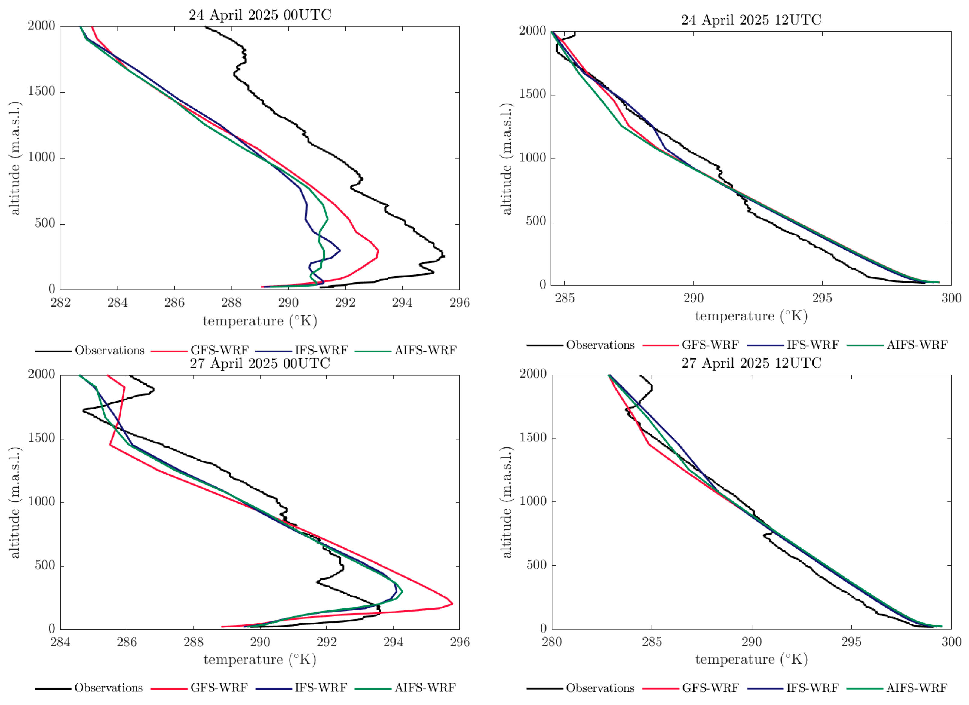
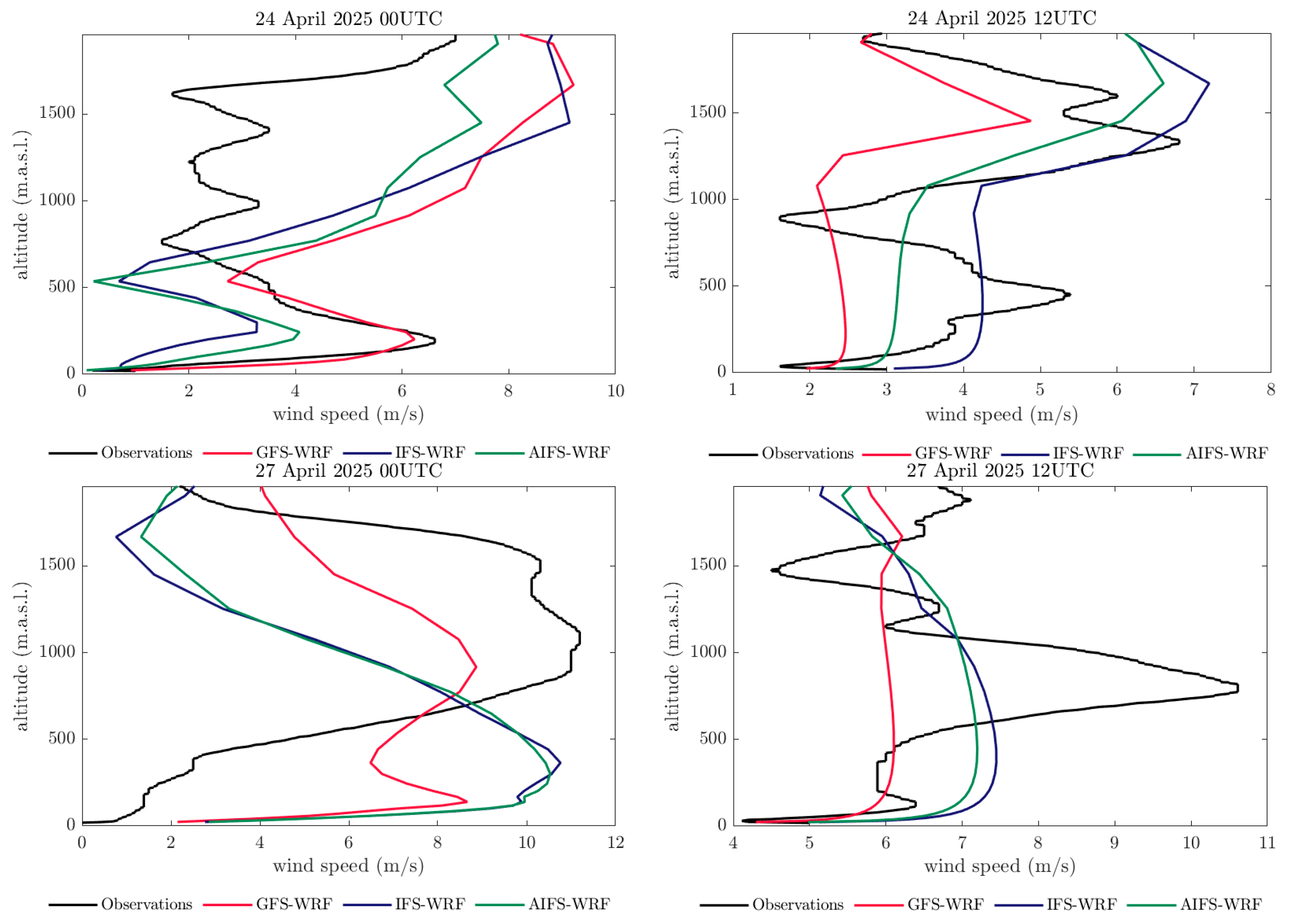
Vertical profiles of temperature (Figure 10) and wind speed (Figure 11) are presented for 24 April and 27 April 2025. These dates were selected for analysis due to the presence of high SO2 concentrations and the identification of notable discrepancies among the WRF simulations. The profiles correspond to results obtained using WRF initialised with different global models (GFS, IFS, and AIFS) within the innermost modelling domain (d03).
Each figure includes a comparison with radiosonde measurements launched from the reference station. The analysis focuses on the Planetary Boundary Layer (PBL) region, given its critical role in pollutant dispersion processes. For accurate interpretation, it is important to note that WRF data are extracted from the vertical column of the grid point closest to the station, whereas the radiosonde drifts horizontally during its ascent. This displacement may introduce slight differences between the modelled and observed profiles.

3.6. Effects over Backward Trajectories

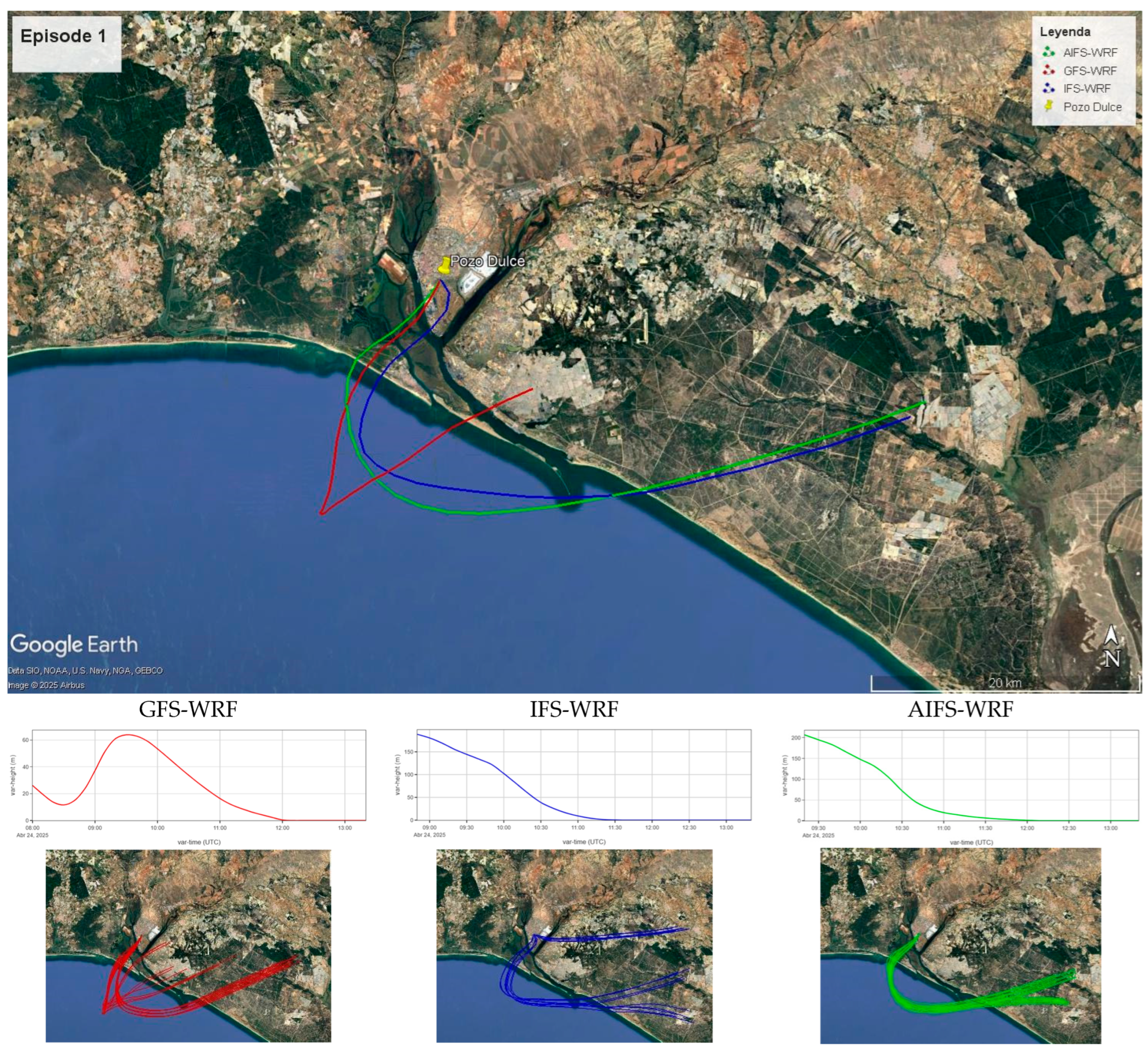
Figure 12 and Figure 13 display backward trajectories for the selected episodes, based on meteorological conditions forecasted by WRF initialised with different global models. All results correspond to the innermost modelling domain (d03).

3.7. Effects on Dispersion Modelling

In Figure 14 dispersion modelling is presented for the episodes selected considering the meteorological conditions forecast by WRF initialised with different global models and results from d03 modelling domain.

3.8. Comparison of Ventilation Index

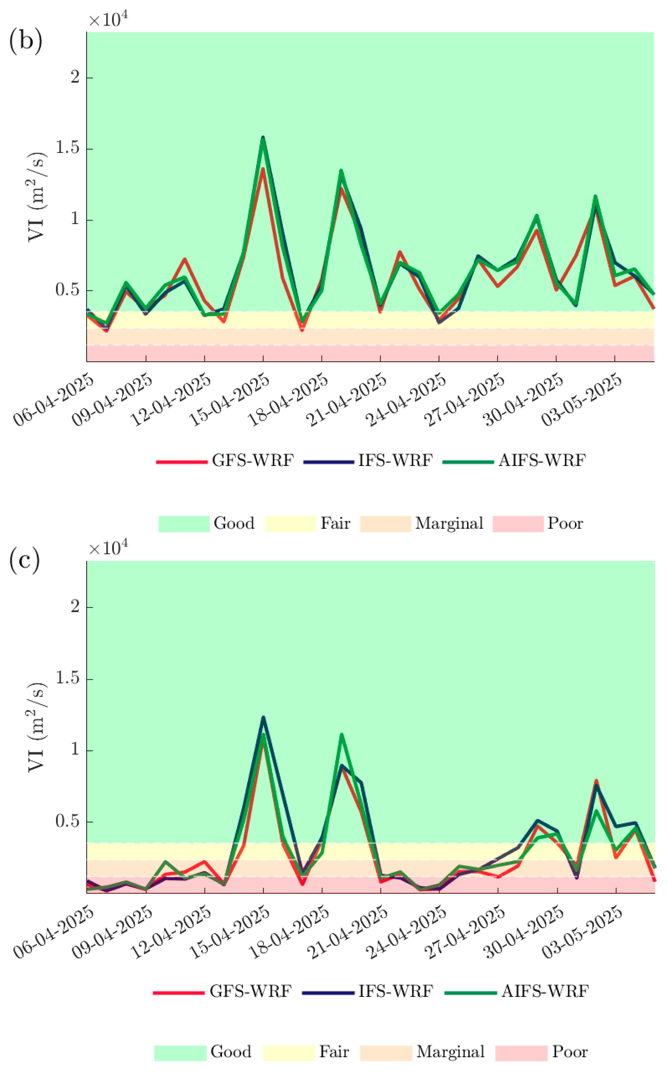
Figure 15 presents the diurnal cycles of the ventilation index (VI) derived from the different WRF simulations. The curves represent the average, maximum, and minimum VI values across all WRF grid cells within the city of Huelva.
Figure 16 shows the diurnal VI values throughout the entire modelling period. In both figures, the classification thresholds defined by [59] are included as reference.

4. Discussion

Given the relatively recent public release of AIFS simulations, no studies have been identified that analyse its coupling with mesoscale models such as WRF, so it has not been possible to compare the results obtained in this research with previous studies. Previous studies identified are related to the comparison between IFS and AIFS simulations. Ref. [17] offers a systematic comparison between AIFS and IFS for different regions around the world, considering different vertical levels, analysis data, and observations, and provides different statistical parameters like RMSE, SDAF and CCAF/SEEPS for different forecast horizons. Using the results generated by [17], it can be observed that, in general, over Europe, AIFS improves IFS results for geopotential, mean sea level pressure, temperature, and wind speed, but there are relevant exceptions. On one hand, at high levels like 50 or 100 hPa, IFS provides better results than AIFS, probably due to the lesser existing instrumental or remote sensing information that feed AIFS. On the other hand, the forecasted values of wind velocity at 10 m by IFS for the next 48–72 h are better than AIFS. Results obtained in this research do not offer significant discrepancies between IFS-WRF and AIFS-WRF, being very similar to the results obtained, in general, for both models.
The deterministic numerical comparison performed in this research reveals that the uncertainty associated with the WRF model is very similar regardless of whether it is initialised with GFS, IFS, or AIFS. For temperature, all three configurations tend to underestimate observed values, particularly during daytime hours. However, WRF initialised with IFS shows slightly better agreement with observations. In contrast, wind speed and direction exhibit negligible differences among the three configurations, although all tend to overestimate wind speed. Relative humidity also shows a marginally better fit with IFS-WRF, though the improvement is minimal. As expected, forecast uncertainty increases with longer forecast horizons (24, 48, and 72 h), but the differences in uncertainty between the three global models, in general, remain small across these horizons. In the case of temperature, it has been identified that the differences between the 48 h versus 24 h forecasts and the 72 h versus 24 h forecasts are more relevant in the case of GFS-WRF and IFS-WRF than in the case of AIFS-WRF. When comparing the 48 h forecast versus 24 h and 72 h versus 24 h temperature, MAGE increases of 5% and 6% are identified for GFS-WRF and IFS-WRF, respectively, while in the case of AIFS-WRF, the difference is practically zero. The results obtained from the deterministic numerical comparison are similar to those obtained in [42] in the same region (Huelva) using GFS as initial conditions and lateral boundary conditions.
The analysis of diurnal cycles provides insight into time-of-day biases in model performance. For temperature, the underestimation is most pronounced during midday, when temperatures peak. At night, coastal stations such as El Arenosillo and Cartaya Pemares show a tendency for the models to overestimate temperature. Wind speed overestimation is most evident in Huelva Ronda Este during daytime hours, while nighttime patterns are more variable, with slight over- and underestimations of light winds. Coastal stations consistently show overestimation throughout the day, particularly in El Arenosillo, with AIFS-WRF producing the highest daytime wind speed overestimation, which may lead to exaggerated horizontal pollutant dispersion. Relative humidity patterns vary by location. In Huelva Ronda Este, underestimation is most pronounced during midday, while coastal stations show overestimation throughout the day. At night, modelled and observed values align closely in Huelva Ronda Este, whereas coastal stations exhibit slight underestimations. These patterns remain consistent across all forecast horizons.
The diurnal evolution of the planetary boundary layer height (PBLH) is well captured by all three WRF configurations, with no significant differences in timing or magnitude. Maximum discrepancies of up to 200 m are observed, likely because PBLH is primarily governed by WRF’s internal physics rather than external initialisation data.
Wind rose analysis reveals subtle differences in wind direction forecasts. While MAGE results are similar across configurations, IFS-WRF and AIFS-WRF produce nearly identical wind roses, both identifying NNW as the dominant wind direction. In contrast, GFS-WRF identifies SSW as dominant and shows a stronger tendency to forecast westerly winds (50%), compared to 48% and 47% for IFS-WRF and AIFS-WRF, respectively. Observations indicate that westerly winds occurred 55% of the time.
Despite the numerical similarity in wind forecasts, visual inspection highlights relevant differences. AIFS-WRF tends to simulate higher wind speeds during daytime hours, with negligible differences at night. Spatially, IFS-WRF and AIFS-WRF show greater consistency with each other than with GFS-WRF, reflecting the inherent similarities between the IFS and AIFS global models. These discrepancies influence the simulation of mesoscale phenomena such as sea breezes and calm zones. For instance, on 27 April 2025, offshore winds reached Huelva at different times, with varying intensities and directions depending on the model (Figure 9). Such differences are particularly relevant for assessing pollutant transport from nearby industrial areas to the urban area.
The geographic distribution of the planetary boundary layer height (PBLH) is found to be very similar across the three WRF configurations. Nonetheless, differences of 100–200 m are identified, although modest in magnitude, may significantly influence pollutant dispersion forecasts when WRF outputs are used as input for dispersion or photochemical models. These variations affect the volume available for mixing pollutants within the convective boundary layer, thereby altering the predicted concentration levels.
The comparison of vertical temperature profiles between WRF simulations and radiosonde data reveals strong agreement at 12 UTC for both analysed episodes. All three configurations diagnose unstable thermal stratification, favouring vertical mixing. However, at 00 UTC, notable discrepancies emerge both among the simulations and in comparison with radiosonde observations. A near-surface temperature inversion is diagnosed at 00 UTC in both episodes, reproduced by GFS-WRF on 24 and 27 April, while IFS-WRF and AIFS-WRF only capture this inversion on 27 April. Additionally, the altitude and intensity of the maximum temperature vary across simulations. For 24 April, IFS-WRF and AIFS-WRF deviate from observed profiles within the first 700–800 m, potentially impacting dispersion forecasts due to the stable stratification associated with thermal inversions.
From the quantitative analysis of numerical validation of the variables temperature and wind velocity at height, and considering, in the analysis, the first eight vertical levels from the Earth’s surface, it is identified that for 24 April at 00 UTC, the GFS-WRF configuration is the one that provides the best results, with values of 0.6 °C and 1.9 m/s of MAGE of temperature and RMSE of wind, respectively, while the values of IFS-WRF and AIFS-WRF are 1.2 °C and more than 3 m/s. This behaviour is also reproduced during the episode of 27 April at 00 UTC, obtaining values of MAGE of temperature of 0.9 °C and RMSE of wind speed of 1.7 m/s for GFS-WRF, while the values for IFS-WRF and AIFS-WRF are 1.2 °C and 2.4 m/s, respectively. However, at 12 UTC, the behaviour is slightly different. The temperature MAGEs for GFS-WRF, IFS-WRF, and AIFS-WRF are 0.7, 0.5, and 0.8 °C, while the wind speed RMSEs are 1.8, 1.3, and 1.3 m/s, respectively, with IFS providing the best results. Similarly, on 27 April at 12 UTC, the temperature MAGEs for GFS-WRF, IFS-WRF, and AIFS-WRF are 0.8, 0.6, and 0.6 °C, while the wind speed RMSEs are 1.8, 1.4, and 1.4 m/s, respectively, with IFS and AIFS providing the best results. In the case of wind velocity, underestimation is identified in almost all cases, except for IFS-WRF on 24 April at 12 UTC, where there is an overestimation of 0.8 m/s. In the case of temperature, mean bias values are very close to zero in almost all cases, except for 24 April at 00 UTC where an underestimation of 0.6, 1.2, and 1.2 °C is identified for GFS-WRF, IFS-WRF and AIFS-WRF, respectively.
Wind speed profiles show greater divergence among simulations and with radiosonde data. On 24 April at 00 UTC, GFS-WRF closely matches radiosonde measurements within the first 500 m, accurately reproducing near-surface wind shear. In contrast, IFS-WRF and AIFS-WRF soften this shear. On 27 April at 00 UTC, significant differences are observed, with IFS-WRF and AIFS-WRF diagnosing wind speed minima above 1500 m, contrary to radiosonde data indicating peak wind speeds at that altitude. At 12 UTC, all models simulate looping vertical wind profiles, with minor differences in maximum intensity (1–2 m/s). Between 100 and 1500 m, the simulations show relatively constant wind speeds, though discrepancies with radiosonde profiles persist.
These differences in wind field representation are reflected in the backward trajectory analyses. While trajectories derived from GFS-WRF, IFS-WRF, and AIFS-WRF are moderately similar, certain episodes reveal substantial divergence, leading to different conclusions regarding emission sources. For instance, in Episode 1 (24 April), all three simulations identify the likely SO2 source as located south of Huelva, near the Odiel River, an area with concentrated industrial activity. However, in Episode 2 (27 April), GFS-WRF again points to southern industrial sources, while IFS-WRF and AIFS-WRF suggest an east–northeast origin, where no major SO2-emitting industries are known. This discrepancy suggests that GFS-WRF may offer a more accurate representation in this case.
Vertical trajectory profiles further highlight differences, particularly between GFS-WRF and IFS/AIFS-WRF, which again show strong internal consistency. These variations, combined with differences in near-surface wind fields and PBLH estimates, explain the divergent results in dispersion modelling (Figure 14). For Episode 1, dispersion forecasts are broadly similar, though maximum hourly concentrations differ: 157 µg/m3 for GFS-WRF, versus 132 and 127 µg/m3 for IFS-WRF and AIFS-WRF, respectively. It means that the concentration diagnosed by IFS and AIFS are 16% and 19%, respectively, lower than those generated when GFS is used, as expected later analysing the meteorological differences identified. In Episode 2, however, the wind field discrepancies lead to markedly different dispersion patterns: GFS-WRF predicts pollutant transport toward Huelva, while IFS-WRF and AIFS-WRF forecast westward and west–northwest dispersion.
Finally, the ventilation index (VI) serves as a clear example of how small differences in meteorological inputs can yield divergent air quality forecasts. Although overall VI patterns are consistent across simulations, GFS-WRF tends to forecast lower VI values, particularly during midday, aligning with its lower wind speed predictions. Diurnal VI analyses reveal days with contrasting ventilation conditions across models. For example, on 17 April, GFS-WRF forecasts marginal ventilation, while IFS-WRF and AIFS-WRF indicate fair conditions. On 27 April (Episode 2), minimum VI values suggest poor ventilation according to GFS-WRF, marginal with AIFS-WRF, and fair with IFS-WRF. These differences could significantly influence the interpretation of pollutant dispersion and exposure risk.
It is important to note that the differences identified in weather forecasts using GFS, IFS, or AIFS with WRF can lead to significant changes in decision-making or air quality management. The different backward trajectories identified during Episode 2 may lead to different identifications of the emission sources responsible for the episode. Or the differences identified in the forecast of ventilation conditions may lead to more or less stringent decisions regarding emission reduction requirements.
The authors want to remark that the comparison between GFS/IFS/AIFS-WRF was made based on publicly available information from the three global models, as the objective was to analyse operational implications. It should be emphasised that the characteristics of the publicly available information at the time of this investigation differed from the three models, both in terms of vertical resolution and time frequency as explained in Section 2.2.2. These differences, given that the global models are being used to initialise a mesoscale model like WRF, are undoubtedly affecting the results obtained in this investigation. If the three global models had at least the same or similar vertical resolution, the differences obtained in the PBL forecast or the wind field would be expected to be smaller.

5. Conclusions

Three global models like GFS, IFS and AIFS have been used as initial and boundary conditions for the mesoscale model WRF. A comparison of the results forecasted for every one of these models has been made, focusing on the meteorological variables that affect air dispersion more. Furthermore, backward trajectory analysis, dispersion modelling and ventilation index have been used as tools to compare the results obtained by every kind of simulation: GFS-WRF, IFS-WRF, and AIFS-WRF. The main conclusions achieved through this research include the following:
  • The choice of the global initialisation model has a minimal impact on overall forecast accuracy for wind speed and wind direction, and only slightly better results have been found for temperature and relative humidity when IFS is used as global initialisation model.
  • Compared to the findings of [42], WRF parameterisations and the use of high-resolution physiographic datasets, such as topography and land use, play a more significant role in the performance of meteorological simulations.
  • Noticeable differences were observed in wind pattern representation and the estimation of the PBLH. These differences, which originate from the global initialisation model, can lead to divergent conclusions regarding pollutant dispersion, the contribution of various emission sources to concentration levels, and decision-making in air quality management.
  • The findings of this research may also support the development of probabilistic air quality forecasting systems based on ensemble approaches.
Some areas of limitations and improvement are identified for this research work. Thus, the following activities are considered for future work:
  • To couple a photochemical model in long-term simulations to assess the impact of different global models used to initialise WRF on air quality forecasts using real local emissions.
  • To evaluate the influence of global model initialisation on other key meteorological variables, such as precipitation.
  • Additionally, future studies could benefit from estimating PBLH using the methodology proposed by [63] and comparing those values with WRF outputs.

Author Contributions

Conceptualisation, R.A.A.; methodology, R.A.A., M.G.-V.O. and M.P.S.; software, M.G.-V.O. and M.P.S.; validation, R.A.A. and M.G.-V.O.; formal analysis, R.A.A.; investigation, R.A.A. and M.G.-V.O.; resources, R.A.A., M.G.-V.O. and M.P.S.; data curation, M.G.-V.O. and M.P.S.; writing—original draft preparation, R.A.A.; writing—review and editing, R.A.A., M.G.-V.O. and B.C.S.; visualisation, R.A.A.; supervision, R.A.A.; project administration, R.A.A.; funding acquisition, R.A.A. and M.G.-V.O. All authors have read and agreed to the published version of the manuscript.

Funding

M.G.-V.O. was supported through a contract funded by project PID2021-126401OB-I00, funded by MICIU/AEI/10.13039/501100011033 and by FEDER, EU.

Data Availability Statement

The datasets presented in this article are not readily available because they are part of an ongoing study.

Acknowledgments

The authors would like to kindly thank Jesús D. de la Rosa of CIQSO/UHU for providing the data from the air quality stations used.

Conflicts of Interest

The authors declare no conflicts of interest.

Abbreviations

The following abbreviations are used in this manuscript:
AEMETNational Spanish Meteorological Agency
AIArtificial Intelligence
AIFSArtificial Intelligence/Integrated Forecasting System
ARWAdvanced Research WRF
CCAFAnomaly Correlation
ECMWFEuropean Centre for Medium-Range Weather Forecasts
ERA5ECMWF Reanalysis v5
GFSGlobal Forecasting System
HYSPLITHybrid Single-Particle Lagrangian Integrated Trajectory
LAMsLimited-Area Models
LBCsLateral Boundary Conditions
m.a.g.lMetres above ground level
m.a.s.lMetres above sea level
MAGEMean Absolute Gross Error
MBMean Bias
NCARNational Center of Atmospheric Research
RMSERoot Mean Square Error
SDAFStandard Deviation of Forecast Anomaly
SEEPSStable Equitable Error in Probability Space
USGSUnited States Geological Survey
UTCUniversal Time Coordinated
VIVentilation Index
WRFWeather Research and Forecasting System

References

  1. EEA. How Air Pollution Affects Our Health; European Environment Agency: Copenhagen, Denmark, 2024; Available online: https://www.eea.europa.eu/en/topics/in-depth/air-pollution/eow-it-affects-our-health (accessed on 28 September 2025).
  2. Directive (EU) 2024/2881 of the European Parliament and of the Council of 23 October 2024 on Ambient Air Quality and Cleaner Air for Europe. Available online: https://eur-lex.europa.eu/eli/dir/2024/2881/oj (accessed on 28 September 2025).
  3. Tritscher, T.; Raz, R.; Levi, Y.; Levy, I.; Broday, D.M. Emissions vs. turbulence and atmospheric stability: A study of their relative importance in determining air pollutant concentrations. Sci. Total Environ. 2020, 733, 139300. [Google Scholar]
  4. Finnish Meteorological Institute. Model Serves its Purposes. Available online: https://en.ilmatieteenlaitos.fi/model-serves-its-purpose (accessed on 28 September 2025).
  5. NOAA. The Global Forecasting System (GFS); NOAA National Centers for Environmental Information: Asheville, NC, USA, 2025. Available online: https://www.emc.ncep.noaa.gov/emc/pages/numerical_forecast_systems/gfs/documentation.php (accessed on 24 March 2025).
  6. ECMWF. IFS Documentation; European Centre for Medium-Range Weather Forecasts: Shinfield Park, UK, 2024; Available online: https://www.ecmwf.int/en/publications/ifs-documentation (accessed on 24 March 2025).
  7. Skamarock, W.C.; Klemp, J.B.; Dudhia, J.; Gill, D.O.; Liu, Z.; Berner, J.; Wang, W.; Powers, J.G.; Duda, M.G.; Barker, D.M.; et al. A Description of the Advanced Research WRF Version 4. In NCAR Technical Note NCAR/TN-556+STR; National Center for Atmospheric Research: Boulder, CO, USA, 2019; p. 145. [Google Scholar] [CrossRef]
  8. Bengtsson, L.; Andrae, U.; Aspelien, T.; Batrak, Y.; Calvo, J.; de Rooy, W.; Gleeson, E.; Hansen-Sass, B.; Homleid, M.; Hortal, M.; et al. The HARMONIE–AROME Model Configuration in the ALADIN-HIRLAM NWP System. Mon. Weather. Rev. 2017, 145, 1919–1935. [Google Scholar] [CrossRef]
  9. Wu, Y.; Xue, W. Data-Driven Weather Forecasting and Climate Modeling from the Perspective of Development. Atmosphere 2024, 15, 689. [Google Scholar] [CrossRef]
  10. Zhang, H.; Liu, Y.; Zhang, C.; Li, N. Machine Learning Methods for Weather Forecasting: A Survey. Atmosphere 2025, 16, 82. [Google Scholar] [CrossRef]
  11. Chadalavada, S.; Faust, O.; Salvi, M.; Seoni, S.; Raj, N.; Raghavendra, U.; Gudigar, A.; Datta, P.; Barua, P.D.; Molinari, F.; et al. Application of artificial intelligence in air pollution monitoring and forecasting: A systematic review. Environ. Model. Softw. 2024, 185, 106312. [Google Scholar] [CrossRef]
  12. Li, Y.; Guo, J.; Sun, S.; Li, J.; Wang, S.; Zhang, S. Air quality forecasting with artificial intelligence techniques: A scientometric and content analysis. Environ. Model. Softw. 2022, 149, 105329. [Google Scholar] [CrossRef]
  13. ECMWF. AIFS: A New ECMWF Forecasting System; European Centre for Medium-Range Weather Forecasts: Reading, UK, 2025; Available online: https://www.ecmwf.int/en/newsletter/178/news/aifs-new-ecmwf-forecasting-system (accessed on 24 March 2025).
  14. Moldovan, G.; Pinnington, E.; Nemesio, A.P.; Lang, S.; Bouallègue, Z.B.; Dramsch, J.; Alexe, M.; Cruz, M.S.; Hahner, S.; Cook, H.; et al. An update to ECMWF’s machine-learned weather forecast model AIFS. arXiv 2025, arXiv:2509.18994v1. [Google Scholar] [CrossRef]
  15. Climate Data Store. ERA5 Hourly Data on Single Levels from 1940 to Present. Available online: https://cds.climate.copernicus.eu/datasets/reanalysis-era5-single-levels?tab=overview (accessed on 16 October 2025).
  16. ECMWF. Implementation of AIFS Single V1; European Centre for Medium-Range Weather Forecasts: Shinfield Park, UK, 2025; Available online: https://confluence.ecmwf.int/display/FCST/Implementation+of+AIFS+Single+v1 (accessed on 26 March 2025).
  17. ECMWF. AIFS-Single Vs. IFS Scorecard; European Centre for Medium-Range Weather Forecasts: Shinfield Park, UK, 2025; Available online: https://sites.ecmwf.int/aifs/scorecards/AIFS-single%20vs%20IFS%20scorecard.html (accessed on 26 March 2025).
  18. Zhang, Z.; Fischer, E.; Zscheischler, J.; Engelke, S. Numerical models outperform AI weather forecasts of record-breaking extremes. arXiv 2025, arXiv:2508.15724. [Google Scholar] [CrossRef]
  19. Figurski, M.J.; Nykie, L.G.; Jaczewski, A.; Baldysz, Z.; Wdowikowski, M. The impact of initial and boundary conditions on severe weather event simulations using a high-resolution WRF model. Case study of the derecho event in Poland on 11 August 2017. Meteorol. Hydrol. Water Manag. 2022, 10, 60–87. [Google Scholar] [CrossRef]
  20. Lang, S.; Alexe, M.; Chantry, M.; Dramsch, J.; Pinault, F.; Raoult, B.; Clare, M.C.A.; Lessig, C.; Maier-Gerber, M.; Magnusson, L.; et al. AIFS—ECMWF’s Data Driven Forecasting System. arXiv 2024, arXiv:2406.01465. [Google Scholar] [CrossRef]
  21. Nipen, T.N.; Haugen, H.H.; Ingstad, M.S.; Nordhagen, E.M.; Salihi, A.F.S.; Tedesco, P.; Seierstad, I.A.; Kristiansen, J.; Lang, S.; Alexe, M.; et al. Regional data-driven weather modeling with a global stretched grid. arXiv 2024, arXiv:2409.02891. [Google Scholar] [CrossRef]
  22. Cesari, R.; Paradisi, P.; Allegrini, P. Source identification by a statistical analysis of backward trajectories based on peak pollution events. Int. J. Environ. Pollut. 2014, 55, 94. [Google Scholar] [CrossRef]
  23. Querol, X.; Alastuey, A.; De la Rosa, J.; Sánchez-de-la-Campa, A.M.; Plana, F.; Ruiz, C.R. Source apportionment analysis of atmospheric particulates in an industrialised urban site in southwestern Spain. Atmos. Environ. 2002, 36, 3113–3125. [Google Scholar] [CrossRef]
  24. Cachorro, V.E.; Toledano, C.; Prats, N.; Sorribas, M.; Mogo, S.; Berjón, A.; Torres, B.; Rodrigo, R.; de la Rosa, J.; De Frutos, A.M. The strongest desert Dust intrusion mixed with smoke over the Iberian Peninsula registered with Sun photometry. J. Geophys. Res. Atmos. 2008, 113, D14. [Google Scholar] [CrossRef]
  25. Sánchez de la Campa, A.M.; De la Rosa, J.; Querol, X.; Alastuey, A.; Mantilla, E. Geochemistry and origin of PM10 in the Huelva región, Southwestern Spain. Environ. Res. 2007, 103, 305–316. [Google Scholar] [CrossRef] [PubMed]
  26. Sánchez de la Campa, A.M.; Sánchez-Rodas, D.; Alsioufi, L.; Alastuey, A.; Querol, X.; de la Rosa, J.D. Air quality trends in an industrialised area of SW Spain. J. Clean. Prod. 2018, 186, 465–474. [Google Scholar] [CrossRef]
  27. Fernández-Camacho, R.; De la Rosa, J.; Sánchez de la Campa, A.M.; González-Castanedo, Y.; Alastuey, A.; Querol, X.; Rodríguez, S. Geochemical characterization of Cu-smelter emission plumes with impact in an urban area of SW Spain. Atmos. Res. 2010, 96, 590–601. [Google Scholar] [CrossRef]
  28. González-Castanedo, G.; Moreno, T.; Fernández-Camacho, R.; Sánchez de la Campa, A.M.; Alastuey, A.; Querol, X.; De la Rosa, J. Size distribution and chemical composition of particulate matter stack emissions in and around a copper smelter. Atmos. Environ. 2014, 98, 271–282. [Google Scholar] [CrossRef]
  29. Chen, B.; Stein, A.F.; Castell, N.; Gonzalez-Castanedo, Y.; de la Campa, A.S.; de la Rosa, J. Modeling and evaluation of urban pollution events of atmospheric heavy metals from a large Cu-smelter. Sci. Total Environ. 2016, 539, 17–25. [Google Scholar] [CrossRef]
  30. Li, J.; Chen, B.; de la Campa, A.M.; Alastuey, A.; Querol, X.; de la Rosa, J.D. 2005–2014 trends of PM10 source contributions in an industrialized area of southern Spain. Environ. Pollut. 2018, 236, 570–579. [Google Scholar] [CrossRef]
  31. Millán-Martínez, M.; Sánchez-Rodas, D.; Sánchez de la Campa, A.M.; Alastuey, A.; Querol, X.; De la Rosa, J.D. Source contribution and origin of PM and arsenic in a complex industrial region (Huelva, SW Spain). Environ. Pollut. 2021, 274, 116268. [Google Scholar] [CrossRef]
  32. López-Cayuela, M.Á.; Córdoba-Jabonero, C.; Bermejo-Pantaleón, D.; Sicard, M.; Salgueiro, V.; Molero, F.; Carvajal-Pérez, C.V.; Granados-Muñoz, M.J.; Comerón, A.; Couto, F.T.; et al. Vertical characterization of fine and coarse dust particles during an intense Saharan dust outbreak over the Iberian Peninsula in springtime 2021. Atmos. Chem. Phys. 2021, 23, 143–161. [Google Scholar] [CrossRef]
  33. Porras, I.; Solé, J.; Marcos, R.; Arasa, R. Meteorological and Climate Modelling Services Tailored to Viticulturists. Atmos. Clim. Sci. 2021, 11, 148–164. [Google Scholar] [CrossRef]
  34. Solé, J.; Arasa, R.; Picanyol, M.; González, M.; Domingo-Dalmau, A.; Masdeu, M.; Porras, I.; Codina, B. Assessment of Climate Change in Nicaragua: Analysis of Precipitation and Temperature by Dynamical Downscaling over a 30-Year Horizon. Atmos. Clim. Sci. 2016, 6, 445–474. [Google Scholar] [CrossRef]
  35. Modi, A.; Harikumar, R.; Nair, T.M.B. Development of an Advance Research WRF-Based Operational Forecast System for Forcing Ocean Models and Evaluation of Its Winds Using Buoys in the Indian Ocean. Weather. Forecast. 2024, 39, 1459–1468. [Google Scholar] [CrossRef]
  36. Yáñez-Morroni, G.; Gironás, J.; Caneo, M.; Delgado, R.; Garreaud, R. Using the Weather Research and Forecasting (WRF) Model for Precipitation Forecasting in an Andean Region with Complex Topography. Atmosphere 2018, 9, 304. [Google Scholar] [CrossRef]
  37. Huang, H.; Qian, Y.; Bisht, G.; Wang, J.; Chakraborty, T.; Hao, D.; Li, J.; Thurber, T.; Singh, B.; Yang, Z.; et al. WRF-ELM v1.0: A regional climate model to study land–atmosphere interactions over heterogeneous land use regions. Geosci. Model Dev. 2025, 18, 1427–1443. [Google Scholar] [CrossRef]
  38. García-Valdecasas, M.; Gámiz-Fortis, S.; Castro-Díez, Y.; Esteban-Parra, M.J. Evaluation of WRF capability to detect try and wet periods in Spain using drought indices. JRG Atmos. 2017, 122, 1569–1594. [Google Scholar] [CrossRef]
  39. Donaire-Montaño, D.; García-Valdecasas Ojeda, M.; Tacoronte, N.; Rosa-Cánovas, J.J.; Castro-Díez, Y.; Esteban-Parra, M.J.; Gámiz-Fortis, S.R. Finding optimal Noah-MP parameterizations for the characterization of surface heat fluxes in the Iberian Peninsula. Atmospheric Res. 2025, 323, 108143. [Google Scholar] [CrossRef]
  40. Oliva, A.S.; García-Valdecasas Ojeda, M.; Arasa Agudo, R. Evaluation of the Sensitivity of the Weather Research and Forecasting Model to Changes in Physical Parameterizations During a Torrential Precipitation Event of the El Niño Costero 2017 in Peru. Water 2025, 17, 209. [Google Scholar] [CrossRef]
  41. Solano-Farias, F.; García-Valdecasas, M.; Donaire-Montaño, D.; Rosa-Cánovas, J.J.; Castro-Díez, Y.; Esteban-Parra, M.J.; Gámiz-Fortis, S.R. Assessment of physical schemes for WRF model in convection-permitting mode over southern Iberian Peninsula. Atmos. Res. 2024, 299, 107175. [Google Scholar] [CrossRef]
  42. Arasa, R.; Porras, I.; Domingo-Dalmau, A.; Picanyol, M.; Codina, B.; González, M.; Piñón, J. Defining a Standard Methodology to Obtain Optimum WRF Configuration for Operational Forecast: Application over the Port of Huelva (Southern Spain). Atmospheric Clim. Sci. 2016, 6, 329–350. [Google Scholar] [CrossRef]
  43. Reboredo, B.; Arasa, R.; Codina, B. Evaluating Sensitivity to Different Options and Parameterizations of a Coupled Air Quality Modelling System over Bogotá, Colombia. Part I: WRF Model Configuration. Open J. Air Pollut. 2015, 4, 47–64. [Google Scholar] [CrossRef]
  44. Arasa, R.; Soler, M.R.; Olid, M. Evaluating the Performance of a Regional-Scale Photochemical Modelling System: Part I. Ozone Predictions. ISRN Meteorol. 2012, 2012, 860234. [Google Scholar] [CrossRef]
  45. Seaman, N.; Gaudet, B.; Zielonka, J.; Stauffer, D. Sensitivity of Vertical Structure in the Stable Boundary Layer to Variations of the WRF Model’s Mellor-Yamada-Janjic Turbulence Scheme. In Proceedings of the 10th WRF Users’ Workshop, Boulder, CO, USA, 23–26 June 2009. [Google Scholar]
  46. De Meij, A.; Ojha, N.; Singh, N.; Singh, J.; Poelman, D.R.; Pozzer, A. The Impact of High-Resolution SRTM Topography and Corine Land Cover on Lightning Calculations in WRF. Atmosphere 2022, 13, 1050. [Google Scholar] [CrossRef]
  47. Lin, Y.; Colle, B.A. A New Bulk Microphysical Scheme That Includes Varying Degree of Riming and Particle Habits. Mon. Weather Rev. 2011, 139, 1036–1047. [Google Scholar] [CrossRef]
  48. Iacono, M.J.; Delamere, J.S.; Mlawer, E.J.; Shephard, M.W.; Clough, S.A.; Collins, W. Radiative Forcing by Long-Lived Greenhouse Gases: Calculations with the AER Radiative Transfer Model. J. Geophys. Res. Atmos. 2008, 113, D13103. [Google Scholar] [CrossRef]
  49. Dudhia, J. Numerical Study of Convection Observed during the Winter Monsoon Experiment Using a Mesoscale Two-Dimensional Model. J. Atmos. Sci. 1989, 46, 3077–3104. [Google Scholar] [CrossRef]
  50. Kain, J.S. The Kain-Fritsch Convective Parameterization: An Update. J. Appl. Meteorol. 2004, 43, 170–181. [Google Scholar] [CrossRef]
  51. Zhang, D.L.; Anthes, R.A. A high-resolution model of the planetary boundary layer—Sensitivity tests and comparisons with SESAME-79 data. J. Appl. Meteorol. 1982, 21, 1594–1609. [Google Scholar] [CrossRef]
  52. Chen, F.; Dudhia, J. Coupling an Advanced Land Surface–Hydrology Model with the Penn State–NCAR MM5 Modeling System. Part I: Model Implementation and Sensitivity. Mon. Wea. Rev. 2001, 129, 569–585. [Google Scholar] [CrossRef]
  53. Hong, S.-Y.; Noh, Y.; Dudhia, J. A New Vertical Diffusion Package with an Explicit Treatment of Entrainment Processes. Mon. Weather Rev. 2006, 134, 2318–2341. [Google Scholar] [CrossRef]
  54. Stein, A.F.; Draxler, R.R.; Rolph, G.D.; Stunder, B.J.B.; Cohen, M.D.; Ngan, F. NOAA’s HYSPLIT atmospheric transport and dispersion modeling system. Bull. Amer. Meteor. Soc. 2015, 96, 2059–2077. [Google Scholar] [CrossRef]
  55. Romero-Macías, E.; Pérez-Vizcaíno, P.; Sánchez de la Campa, A.; Sánchez- Rodas, D.A.; Alastuey, A.; Querol, X.; De la Rosa, J.D. Extreme historic SO2 levels in an industrial city (Huelva, SW Spain). Air quality implications. RICTA. In Proceedings of the Poster Presented on the 8th Iberian Meeting on Aerosol Science and Technology, A Coruña, Spain, 26–28 June 2024. [Google Scholar]
  56. Pérez-Vizcaíno, P.; Sánchez de la Campa, A.M.; Sánchez-Rodas, D.; De la Rosa, J.D. Application of a near real-time technique for the assessment of atmospheric arsenic and metals emissions from a copper smelter in an urban area of SW Europe. Environ. Pollut. 2025, 367, 125602. [Google Scholar] [CrossRef] [PubMed]
  57. Pronóstico de Ventilación. Ministerio del Medio Ambiente, Gobierno de Chile. Available online: https://airecqp.mma.gob.cl/pronostico-de-ventilacion/ (accessed on 13 August 2025).
  58. Clearing Index. National Weather Service. Available online: https://www.weather.gov/slc/clearingindex (accessed on 13 August 2025).
  59. Ferguson, S.A.; McKay, S.J.; Nagel, D.E.; Piepho, T.; Rorig, M.L.; Anderson, C.; Kellogg, L. Assessing Values of Air Quality and Visibility at Risk from Wildland Fires; US Department of Agriculture, Forest Service, Pacific Northwest Research Station: Portland, OR, USA, 2003; p. 59.
  60. Air Quality Network of the Andalusian Government. Available online: https://www.juntadeandalucia.es/medioambiente/portal/landing-page-%C3%ADndice/-/asset_publisher/zX2ouZa4r1Rf/content/localizaci-c3-b3n-de-la-red-autom-c3-a1tica-de-calidad-del-aire/20151 (accessed on 26 May 2025).
  61. AEMET. Borrascas Con Gran Impacto 2024–2025. Available online: https://www.aemet.es/es/conocermas/borrascas/2024-2025 (accessed on 14 August 2025).
  62. AEMET. Climatological Summaries. Andalusia. Available online: https://www.aemet.es/documentos/es/serviciosclimaticos/vigilancia_clima/resumenes_climat/ccaa/andalucia-ceuta-melilla/avance_climat_acm_abr_2025.pdf (accessed on 5 August 2025).
  63. Comas Muguruza, A.; Arasa Agudo, R.; Udina, M. Characterization of the Planetary Boundary Layer Height in Huelva (Spain) During an Episode of High NO2 Pollutant Concentrations. Earth 2025, 6, 26. [Google Scholar] [CrossRef]
  64. Abida, R.; Addad, Y.; Francis, D.; Temimi, M.; Nelli, N.; Fonseca, R.; Nesterov, O.; Bosc, E. Evaluation of the Performance of the WRF Model in a Hyper-Arid Environment: A Sensitivity Study. Atmosphere 2022, 13, 985. [Google Scholar] [CrossRef]
  65. Rzeszutek, M.; Kłosowska, A.; Oleniacz, R. Accuracy Assessment of WRF Model in the Context of Air Quality Modeling in Complex Terrain. Sustainability 2023, 15, 12576. [Google Scholar] [CrossRef]
  66. Emery, C.; Tai, E. Enhanced Meteorological Modeling and Performance Evaluation for Two Texas Ozone Episodes; Texas Natural Resources Conservation Commission: Novato, CA, USA, 2001.
  67. Tesche, T.W.; McNally, D.E.; Tremback, C. Operational Evaluation of the MM5 Meteorological Model over the Continental United States: Protocol for Annual and Episodic Evaluation; Alpine Geophysics, LLC.: Boulder, CO, USA, 2002; Available online: http://www.epa.gov/scram001/reports/tesche_2002_evaluation_protocol.pdf (accessed on 27 May 2025).
  68. Jiménez, P.A.; González-Rouco, J.F.; García-Bustamante, E.; Navarro, J.; Montávez, J.P.; Vilà-Guerau de Arellano, J.; Dudhia, J.; Roldán, A. Surface Wind Regionalization over Complex Terrain: Evaluation and Analysis of a High-Resolution WRF Numerical Simulation. J. Appl. Meteorol. Climatol. 2010, 49, 268–287. [Google Scholar] [CrossRef]
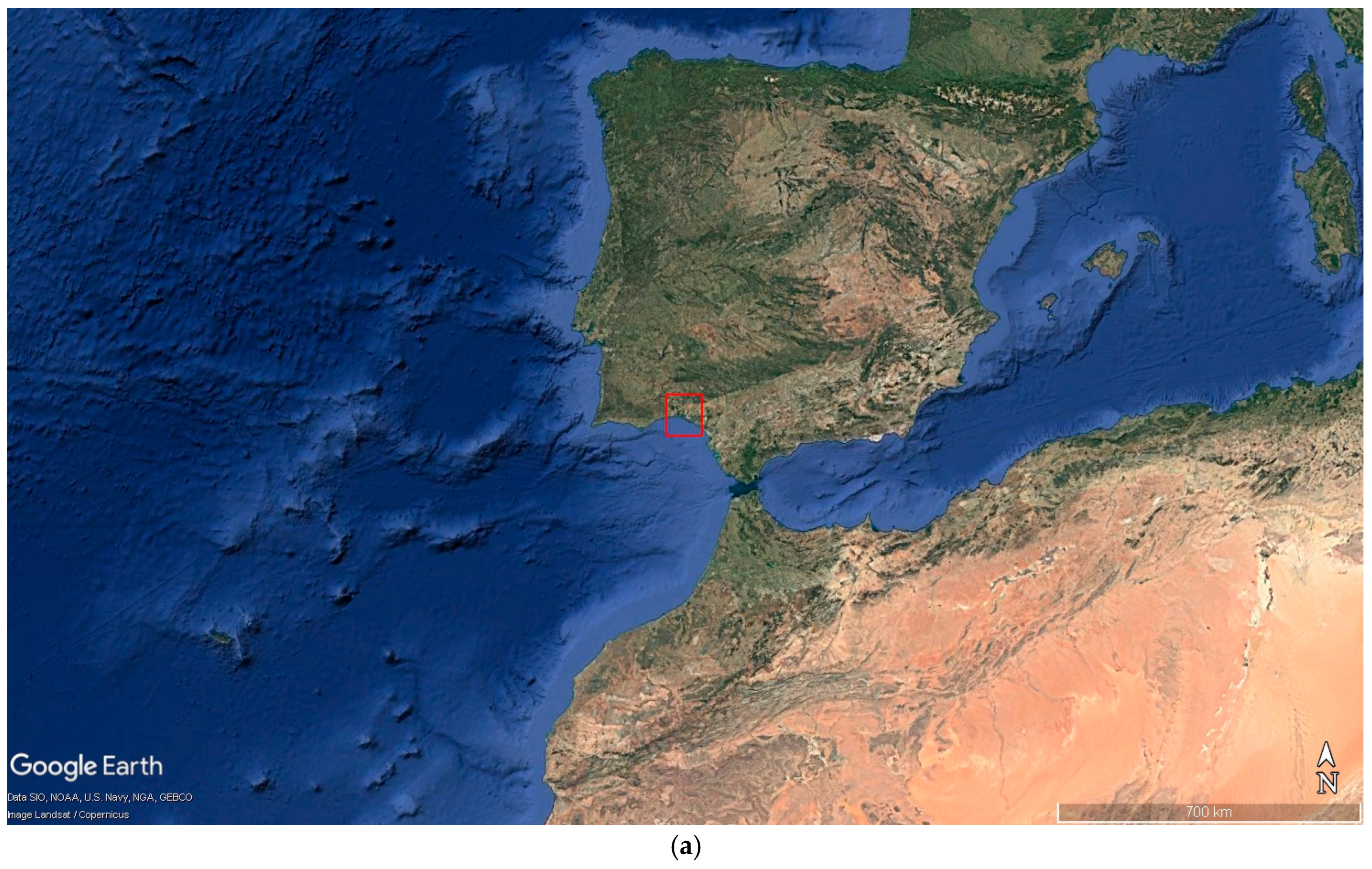
Figure 1. (a) Geographical location of Huelva in the Iberian Peninsula as well as locations (b) of meteorological (in blue) and air quality stations (in yellow) used in this study, radiosounding station (in red) and the location of an imaginary point emission source (in green). (c) A zoom of the city of Huelva and surroundings is included. [Images generated using Google Earth].
Earth 06 00132 g001aEarth 06 00132 g001b
Figure 2. Modelling domains for simulations. [Images generated using Google Earth].
Earth 06 00132 g002
Figure 3. Evolution of 10 min SO2 concentrations during the hours preceding and following selected episodes: Episode 1 (left), Episode 2 (right). Time is expressed in local time (UTC + 2).
Earth 06 00132 g003
Figure 4. Diurnal cycles of observed and modelled temperature, wind speed, and relative humidity at official meteorological stations, averaged across the 24, 48, and 72 h forecast horizons.
Earth 06 00132 g004aEarth 06 00132 g004b
Figure 5. Diurnal cycles of modelled planetary boundary layer height (PBLH) at the official meteorological station of Huelva Ronda Este, corresponding to the 24 h forecast horizon.
Earth 06 00132 g005
Figure 6. Wind roses of observed and modelled values at the official meteorological station of Huelva Ronda Este. It should be noted that the information provided by AEMET (observed information) is every 45 degrees.
Earth 06 00132 g006
Figure 7. Forecast maps of PBLH under different meteorological modelling conditions (GFS-WRF, IFS-WRF, and AIFS-WRF), for domain d03 and a 24 h forecast horizon. The maps correspond to 24 April 2025 at 3 p.m. (left) and 27 April 2025 at 3 p.m. (right).
Earth 06 00132 g007
Figure 8. The same as Figure 7, but for wind speed and wind direction.
Earth 06 00132 g008
Figure 9. Forecast maps of wind speed and wind direction under three meteorological modelling configurations (GFS-WRF, IFS-WRF, and AIFS-WRF), for domain d03 and a 24 h forecast horizon. The maps correspond to 27 April 2025, showing the wind field evolution between 11 am and 2 p.m.
Earth 06 00132 g009
Figure 10. Vertical profiles of temperature considering different meteorological modelling conditions (GFS-WRF, IFS-WRF, and AIFS-WRF) and the radiosonde ascent (observations).
Earth 06 00132 g010
Figure 11. Vertical profiles of wind speed considering different meteorological modelling conditions (GFS-WRF, IFS-WRF, and AIFS-WRF) and the radiosonde ascent (observations).
Earth 06 00132 g011
Figure 12. Normal (top) and ensemble (bottom) backward trajectories generated from different air quality stations during Episode 1 considering different meteorological modelling conditions: GFS-WRF (red), IFS-WRF (blue) and AIFS-WRF (green). It is also included the vertical analysis of the backward trajectory for every WRF model configuration. Images generated using Google Earth.
Earth 06 00132 g012
Figure 13. The same as Figure 12, but for Episode 2.
Earth 06 00132 g013
Figure 14. SO2 surface concentration at 3 p.m. generated from a non-real emission source during the two episodes selected, 24 April 2025, above and 27 April 2025, below, considering different meteorological modelling conditions, GFS-WRF, IFS-WRF and AIFS-WRF. A point emission source at 10 m.a.g.l was considered emitting 40 g/s for 1 h and starting at 2 p.m.
Earth 06 00132 g014aEarth 06 00132 g014b
Figure 15. Diurnal cycles of modelled ventilation index (VI) values for the city of Huelva, based on a 24 h forecast horizon. Plots (a), (b), and (c), respectively, show the spatially calculated maximum, average, and minimum VI values across all WRF grid cells within the urban area.
Earth 06 00132 g015aEarth 06 00132 g015b
Figure 16. Diurnal modelled ventilation index (VI) values for the city of Huelva throughout the analysis period, based on a 24 h forecast horizon. Plots (a), (b), and (c), respectively, show the spatially calculated maximum, average, and minimum VI values. For each day, the VI corresponds to the highest hourly value observed across the modelling domain.
Earth 06 00132 g016aEarth 06 00132 g016b
Table 2. Statistics used for forecast evaluation and corresponding benchmark values. These values are established for flat terrain conditions and can be relaxed with complex topography [42].
Meteorological Variable (Reference Height)Statistic Parameter (Benchmark)
Temperature (2 m)MB (<±0.5 K)
MAGE (<2 K)
IOA ≥ 0.80
Wind Speed (10 m)MB (<±0.5 m/s)
RMSE (<2 m/s)
Wind Direction (10 m)MB (<±10°)
MAGE (<30°)
Relative Humidity (2 m) MB (<±10%)
MAGE (<20%)
IOA ≥ 0.60
Table 3. Numerical evaluation of the different simulations performed over the d03 modelling domain, considering forecast horizons of 24, 48, and 72 h. In bold are the values that comply with the recommendations of [64,67] strictly. Note that AEMET observation values are every 45 degrees and that the recommendations used are valid for areas of simple topography.
Meteorological Parameter (Reference Height)Statistic Parameter (Benchmark)GFS-WRFIFS-WRFAIFS-WRFGFS-WRFIFS-WRFAIFS-WRFGFS-WRFIFS-WRFAIFS-WRF[Units]
24 h24 h24 h48 h48 h48 h72 h72 h72 h
Temperature (2 m)MB < ±0.5 K−1.3−0.6−0.9−1.4−0.7−0.9−1.3−0.7−0.9K
MAGE < 2 K1.91.61.82.01.71.82.01.71.8K
IOA ≥ 0.800.680.730.710.680.720.710.680.720.71--
Wind Speed (10 m)MB < ±0.5 m/s1.41.51.41.21.41.41.31.41.4m/s
RMSE < 2 m/s2.32.42.32.32.42.32.32.42.3m/s
Wind Direction (10 m)MB < ±10°212119232121232121°
MAGE < 30°494949505050515151°
Relative Humidity (2 m) MB < ±10%1.81.62.01.91.61.91.71.51.8%
MAGE < 20%8.57.98.28.78.08.48.88.18.4%
IOA ≥ 0.600.670.690.680.660.680.680.650.680.67--
Disclaimer/Publisher’s Note: The statements, opinions and data contained in all publications are solely those of the individual author(s) and contributor(s) and not of MDPI and/or the editor(s). MDPI and/or the editor(s) disclaim responsibility for any injury to people or property resulting from any ideas, methods, instructions or products referred to in the content.