Article

Predictive Analysis of Hydrological Variables in the Cahaba Watershed: Enhancing Forecasting Accuracy for Water Resource Management Using Time-Series and Machine Learning Models

by
Sai Kumar Dasari
1,
Pooja Preetha
2,* and
Hari Manikanta Ghantasala
3
1
Department of Computer Science Engineering, Alabama A&M University, Huntsville, AL 35811, USA
2
Department of Mechanical and Civil Engineering and Construction Management Alabama A&M University, Huntsville, AL 35811, USA
3
Moschip Technologies Pvt Ltd., Hyderabad 500081, India
*
Author to whom correspondence should be addressed.
Earth 2025, 6(3), 89; https://doi.org/10.3390/earth6030089 (registering DOI)
Submission received: 27 May 2025 / Revised: 19 July 2025 / Accepted: 29 July 2025 / Published: 4 August 2025

Abstract

This study presents a hybrid approach to hydrological forecasting by integrating the physically based Soil and Water Assessment Tool (SWAT) model with Prophet time-series modeling and machine learning–based multi-output regression. Applied to the Cahaba watershed, the objective is to predict key environmental variables (precipitation, evapotranspiration (ET), potential evapotranspiration (PET), and snowmelt) and their influence on hydrological responses (surface runoff, groundwater flow, soil water, sediment yield, and water yield) under present (2010–2022) and future (2030–2042) climate scenarios. Using SWAT outputs for calibration, the integrated SWAT-Prophet-ML model predicted ET and PET with RMSE values between 10 and 20 mm. Performance was lower for high-variability events such as precipitation (RMSE = 30–50 mm). Under current climate conditions, R2 values of 0.75 (water yield) and 0.70 (surface runoff) were achieved. Groundwater and sediment yields were underpredicted, particularly during peak years. The model’s limitations relate to its dependence on historical trends and its limited representation of physical processes, which constrain its performance under future climate scenarios. Suggested improvements include scenario-based training and integration of physical constraints. The approach offers a scalable, data-driven method for enhancing monthly water balance prediction and supports applications in watershed planning.

1. Introduction

Understanding and predicting hydrological variables such as evapotranspiration, surface runoff, groundwater levels, water yield, and sediment transport is crucial for effective water resource management [1]. These variables represent key components of the hydrological cycle and directly influence water availability, agricultural productivity, ecosystem stability, and flood or drought resilience [2,3]. For instance, potential evapotranspiration (PET) and actual evapotranspiration (ET) are widely recognized as vital indicators of atmospheric water demand and plant water usage, which significantly affect both irrigation planning and drought assessments [4]. Time-series forecasting has emerged as a powerful tool in hydrological modeling, especially when long-term historical datasets are available. Traditional statistical models like the autoregressive integrated moving average (ARIMA) have been extensively used but often struggle with missing data and complex seasonality [5]. To address these challenges, more adaptive models such as Facebook Prophet have gained attention in recent years due to their ability to automatically handle outliers, missing values, and strong seasonal patterns. Studies demonstrated Prophet’s robustness in producing interpretable and accurate forecasts in domains with irregular time series, making it a viable option for hydrological forecasting [6]. In hydrological contexts, Prophet has been used to forecast streamflow, rainfall patterns, and temperature variations with promising results [7,8]. Its ability to model each variable independently monthly offers both flexibility and granularity in understanding long-term hydrological trends.
Beyond time-series analysis, machine learning (ML) techniques have increasingly been adopted to model nonlinear relationships in hydrological systems. Techniques such as multi-output regression, support vector machines, and random forests have been employed to capture the complex dependencies between climatic inputs, such as precipitation and temperature, and hydrological outputs, such as stream flows, groundwater recharges, and water yields [9,10,11,12,13]. Multi-output regression allows simultaneous prediction of multiple dependent variables, improving coherence across interconnected hydrological parameters. Meanwhile, polynomial feature transformations help in capturing higher-order interactions between features, enhancing model expressiveness in physically complex systems [14]. These hybrid approaches of merging time-series models with ML have been proven to outperform single-model strategies, particularly in applications involving sediment transport, runoff prediction, and water use forecasting [15].
Data quality plays a critical role in the success of hydrological forecasting. Proper data preprocessing, including cleaning, outlier removal, and handling of missing values, is essential for minimizing model bias and improving generalization [16,17]. The study’s use of time-series models required transforming the dataset into a suitable structure, with each hydrological variable modeled independently, allowing for a clearer understanding of variable-specific patterns. For evaluating model performance, metrics such as the Mean Absolute Error (MAE), Mean Squared Error (MSE), Root Mean Squared Error (RMSE), Nash Sutcliffe efficiency (NSE), and coefficient of determination (R2) are commonly applied in regression-based hydrological studies [18]. These metrics offer quantifiable insight into prediction accuracy and the degree of explained variance, which are critical for validating model reliability in planning scenarios for effective water resources management. Such integration of forecasted hydrological insights into water resource management has significant real-world implications. Forecasting tools are increasingly being used by policymakers and planners to support water allocation, disaster risk reduction, and sustainable development strategies for water use management. Accurate predictions of water yield and runoff patterns can aid in designing efficient irrigation systems, while sediment yield forecasts can inform erosion control and reservoir management practices [19]. Furthermore, predictive analytics enable the early identification of hydrological extremes, supporting timely interventions in flood-prone or drought-susceptible regions [20]. As climate change introduces more uncertainty into hydrological systems, data-driven approaches are becoming indispensable for building resilient water governance frameworks [21,22].
The vital contribution of this study lies in its integrated approach to predictive hydrological modeling, combining the strengths of time-series forecasting using the Prophet model with machine learning techniques such as multi-output regression and polynomial feature transformations. By leveraging historical hydrological data from 2005 to 2022 in the Cahaba watershed, the research advances the existing literature through precise monthly forecasting of key environmental variables, including precipitation, snowmelt, evapotranspiration, and potential evapotranspiration, and their influence on hydrological responses of surface runoff, groundwater flow, soil water content, sediment yield, and overall water yield. Unlike traditional models that often treat these variables in isolation, this study offers a comprehensive framework that captures complex, nonlinear interactions between inputs and outputs. The comparative analysis between Prophet-based predictions and SWAT model outputs under both present and future climate scenarios not only validates the forecasting methods but also provides actionable insights for sustainable water resource management and climate adaptation.
Despite the growing application of hybrid models in hydrological forecasting, there remains a critical gap in integrating physically based models with time-series decomposition techniques that retain seasonal structure while enabling nonlinear response estimation. The existing literature often applies machine learning models directly to raw hydrological data or SWAT outputs, which can lead to poor generalization, especially in the presence of high-frequency noise or complex seasonality [23]. This study addresses this gap by introducing a novel SWAT-Prophet-ML framework that leverages the structural interpretability of Prophet for trend and seasonality extraction from SWAT-generated water balance variables and uses those outputs as features in a multi-output regression model with polynomial transformations to predict key hydrological responses. This two-stage decomposition regression pipeline enhances feature expressiveness while reducing the complexity typically faced in fully empirical models. Innovation lies not in the use of individual tools such as SWAT, Prophet, or ML but in methodological synergy. Prophet helps transform temporally structured but noisy SWAT outputs into stable, decomposed series that improve machine learning performance in multi-variable regression. Furthermore, this model provides a foundation for modular extensions, such as scenario-based training for future climate adaptation, and allows for flexibility in physical-data integration [24].

2. Data and Methods

2.1. Methodology for Hybrid Model Design

The hybrid model proposed in this study, SWAT-Prophet-ML, follows a deliberate design logic aimed at balancing physical realism with data-driven flexibility. The SWAT model serves as a physically based simulation platform for capturing hydrological processes across the watershed, ensuring that baseline outputs (evaporation, snowmelt, precipitation) reflect real-world watershed dynamics under observed climate and land conditions.
The Prophet model is used not for forecasting in isolation, but as a preprocessing mechanism to decompose these SWAT outputs into trend and seasonal components. This step offers two distinct advantages: (1) It reduces high-frequency variability and captures domain-relevant periodic behavior, and (2) it provides structured input features that enhance the performance and stability of the subsequent machine learning model. Direct use of raw SWAT outputs in regression often introduces noise and undermines model accuracy, particularly in capturing multi-output hydrological responses like surface runoff, groundwater contribution, or sediment yield. Finally, multi-output regression with polynomial features is employed to learn complex nonlinear mappings between decomposed water balance variables and hydrological responses. Polynomial transformations improve the representational capacity of the model without overfitting to noise, and multi-output regression preserves interdependence among output variables, a common challenge in traditional single-output ML models. This sequential approach—physics-informed simulation → structured decomposition → nonlinear learning—was chosen specifically to balance forecast stability, interpretability, and generalization, especially for applications in watershed-scale water resource planning.
This research contributes a scalable, data-driven methodology that can inform policy and planning decisions in hydrologically sensitive and climate-vulnerable regions. The objectives of the study are
(A)
Apply the Prophet time-series forecasting model to predict key hydrological variables and analyze annual variations for better understanding of climate-driven hydrological patterns.
(B)
To integrate machine learning models (multi-output regression with polynomial features) into Prophet time-series forecasting models to better understand the complex relationships between hydrological input and output variables.
(C)
To validate and evaluate the performance of predictive models by comparing Prophet-machine learning model outputs with SWAT model simulations in the Cahaba watershed.
(D)
Perform comparative analysis of predicted vs. actual water balance components and hydrological responses under both present (2010–2022) and future (2030–2042) climate scenarios in the Cahaba watershed.
The flowchart illustrates the full process for hydrological predictions using time-series forecasting (Prophet) and machine learning models, including data cleaning, forecasting, evaluation, and output generation (Figure 1).

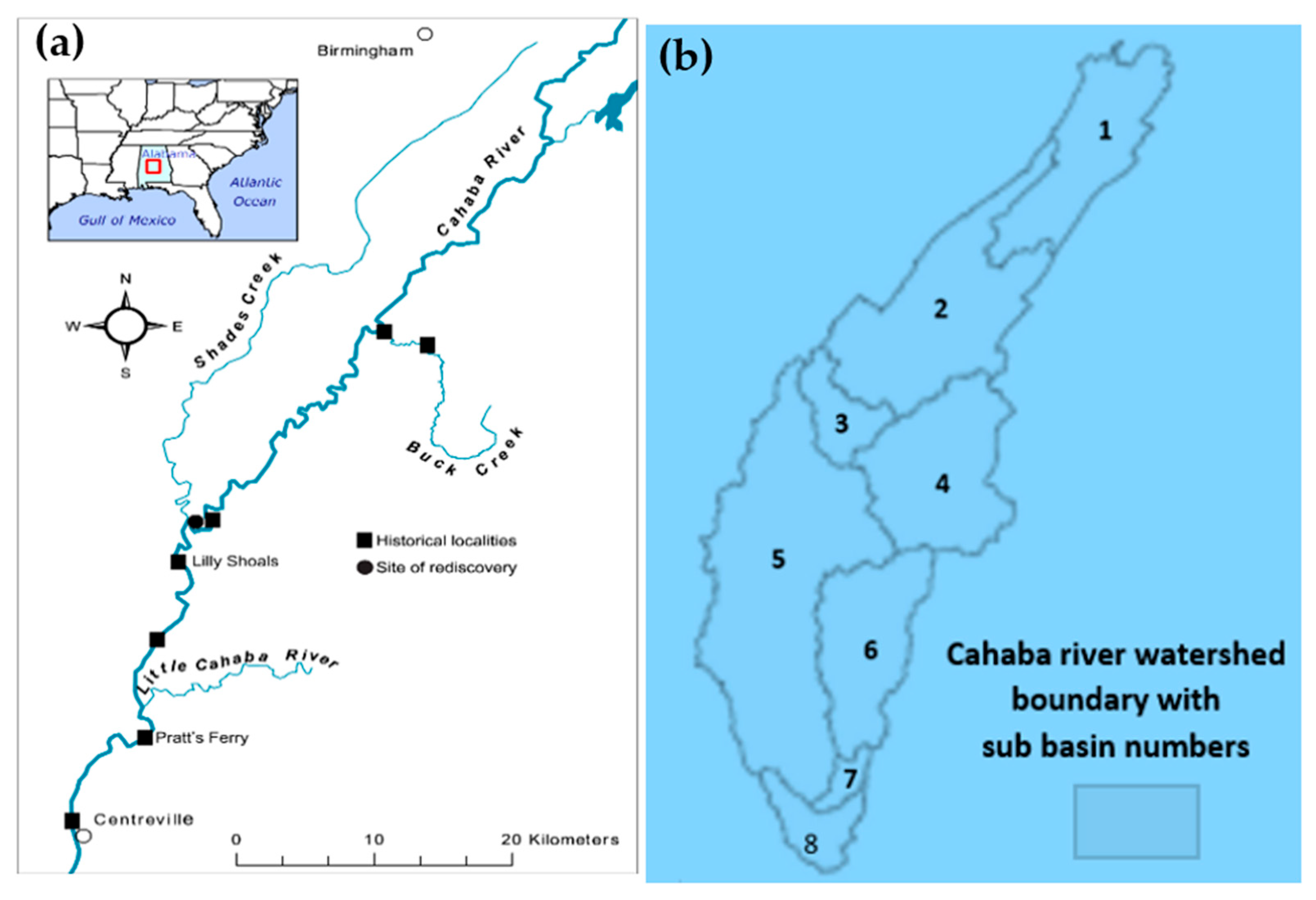
2.2. Study Area and Benchmark Modeling with SWAT Model

A SWAT model was developed for the Cahaba River Basin to simulate hydrological processes under varying land use and climate conditions (Figure 2a). Watershed delineation was conducted using a stream definition threshold of 450 km2, resulting in the identification of eight sub-basins across the river system (Figure 2b). To optimize model efficiency and reduce computational complexity, thresholds for the minimum area were applied during the definition of Hydrologic Response Units (HRUs). In alignment with recent approaches that emphasize high-resolution land cover mapping and the accurate representation of complex land systems [25], certain Land-Use/Land-Cover (LULC) classes were exempted from area thresholding during HRU definition [26]. These included open space development, low-intensity development, medium-intensity development, high-intensity development, and barren land, ensuring that small yet hydrologically significant urban and dryland patches were retained in the simulation.
The area threshold for watershed delineation is 1000 ha and the percentage threshold values for the soil, slope, and land use that were used to define the hydrological response units are 10%, 10%, and 5% respectively. As a result, a total of 78 HRUs were delineated across the eight sub-basins. Model simulations were conducted using LULC datasets for the year 2011 and the model was calibrated to match the real watershed conditions for surface runoff, groundwater storage, and sediment yields (Table 1). Monthly calibration simulations were conducted from November 2013 to October 2017, with the first two years used as a warm-up period (NYSKIP = 2) under a skewed normal rainfall distribution. Streamflow data from the Trussville station, representing the outlet of sub-basin 1 (including HRUs 1–5), was used for calibration and validation. The model inputs fed to the SWAT model and the model outputs retrieved from the calibrated and validated SWAT model are fed as inputs to the Prophet library for time-series forecasting [27].
SWAT handles spatial heterogeneity using Hydrologic Response Units (HRUs), which are unique combinations of land use, soil type, and slope within each sub-basin. This allows the model to simulate distinct vegetation and soil interactions within a watershed, thereby capturing the influence of vegetation heterogeneity on soil moisture dynamics. SWAT uses a multi-layer soil profile that typically includes 1 to 10 layers, with the number and depth of layers defined based on the soil input data. Each layer has its own physical properties, such as texture, hydraulic conductivity, and available water capacity, which influence water movement and storage. In our study, we used the first four layers as per the web soil survey-based soil database, ensuring adequate representation of vertical soil heterogeneity. Vegetation influences soil moisture through evapotranspiration and root zone depth. SWAT controls these processes through vegetation indices that vary by land cover type and soil type. Thus, areas with different vegetation types and growth conditions exhibit distinct soil moisture patterns captured by the HRUs of the Cahaba watershed.

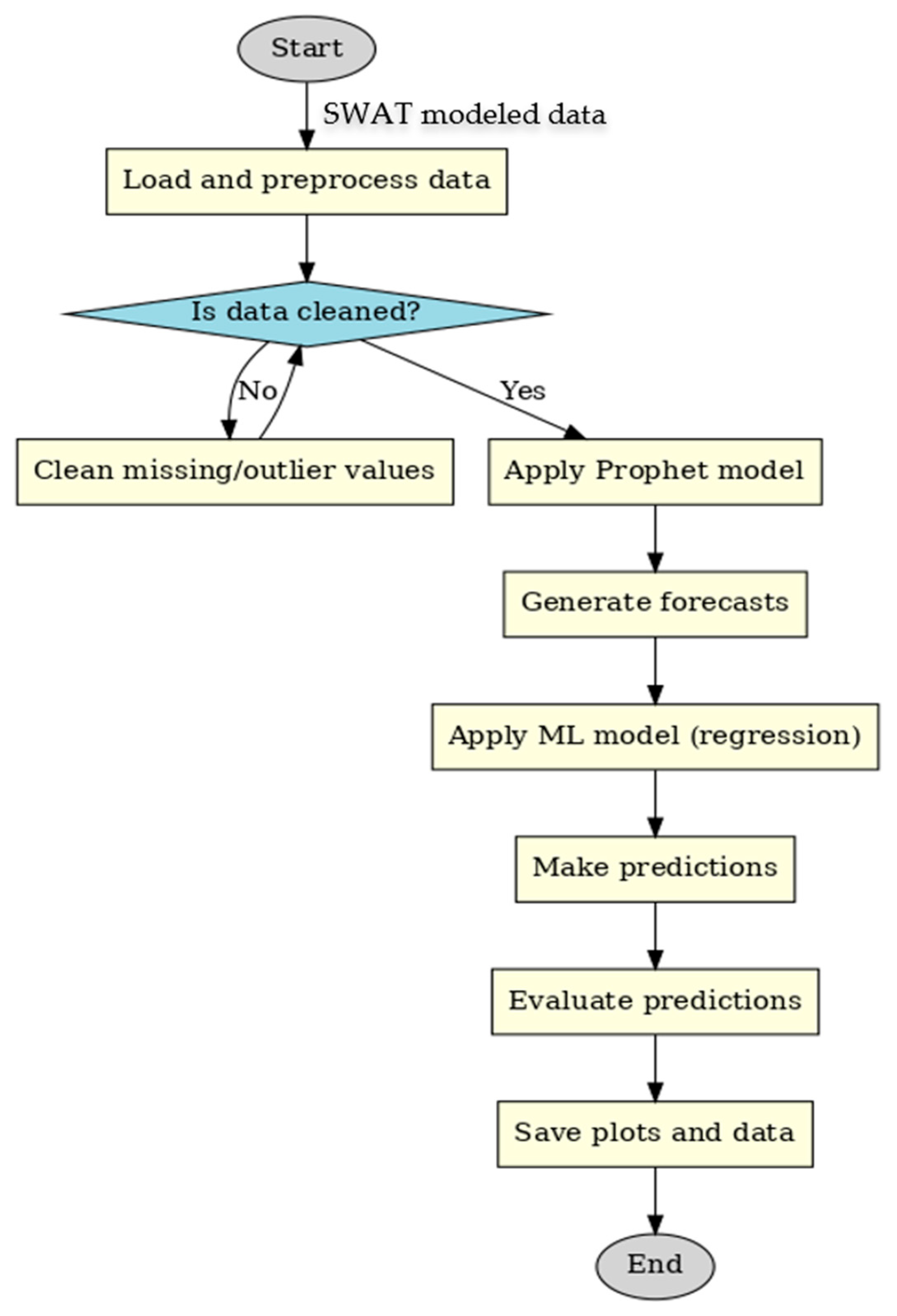
2.3. Hydrological Data Predictions Using Prophet Library

The datasets retrieved form SWAT modeling are loaded from an Excel file named Cahaba-2010–2022-Subbasin1-yields.xlsx. The YEAR and MON columns were combined to create a Year Month datetime format, facilitating time-series analysis. The prediction process involves using the Prophet library, a powerful tool for time-series forecasting and specifies the list of variables to be used in the prediction models. For each variable, a subset of the data containing the year, month, and the variable of interest was prepared, and missing values were dropped. The dataset was reformatted to match Prophet’s requirements, renaming columns to ds (date) and y (target variable). A new Prophet model was instantiated and fitted using the prepared data. The model was used to generate future predictions with monthly frequency, allowing for an analysis of seasonal trends and long-term variability [28].
The predicted values were extracted and cleaned by ensuring no negative predictions, reflecting realistic environmental conditions. The water balance variables, such as precipitation (PRECIPmm in mm), snowmelt contribution (SNOWMELTmm in mm), potential evapotranspiration (PETmm in mm), and evapotranspiration (ETmm in mm), were trained using historical data, and future predictions were generated. Likewise, the output variables, such as the surface runoff contribution to stream flows (SURQmm in mm), groundwater discharge to streams (GW Qmm in mm), soil water content (SWmm in mm), water yield (WYLDmm in mm), and sediment yield (SYLDt_ha in ton/ha), were evaluated for present and future settings. Each variable was modeled individually and predictions for each variable were stored in individual data frames for further processing. To analyze the overall hydrological behavior, the individual predictions were combined into a single data frame. This merging process allows for a comprehensive understanding of how these variables interact and change over time. To evaluate the performance of the forecasting model and understand the dynamics of hydrological variables, actual measurements were merged with the predicted values. This merging process aligns the observed and forecasted data by date, allowing for direct comparison. To compare the real and predicted values of important hydrological variables, separate plots were made for each variable. The visuals show line plots for both actual and predicted values, plus a bar plot that displays prediction errors. These predictive insights can serve as valuable tools in combating the challenges posed by climate change, such as droughts, flooding, and shifts in snowmelt patterns, enabling proactive decision-making for sustainable development [29].

2.4. Time-Series Forecasting with Prophet Model

Prophet is an open-source forecasting tool developed by Facebook, designed to handle time-series data that exhibit trends and seasonality. It is particularly well suited for forecasting with daily observations and can incorporate holidays and other special events into the model. Prophet nonlinear trends are fitted with daily, weekly, and yearly seasonality, including the effects of holidays. The Prophet model not only forecasts the future but also fills missing values and detects irregularities. Although the trend forecast appears reasonable, the uncertainty intervals appear to be too large. The Prophet model can deal with historical outliers, but only by matching them to trend changes. Then, the model predicts similar magnitude trend changes in the future. Outliers are best dealt with by removing them, and the Prophet model has no issues with missing data. If we leave the dates in the future, but we set their values to N/A in history, the Prophet model makes a forecast for their values. In the case of the Prophet model, we also used the maximum likelihood method to estimate its parameters. In this investigation, we have not considered the non-periodic changes in the time series. The Prophet model can handle the time series and automatically bifurcate the future trend (Figure 3).
A Prophet model is formulated as
Y(t) = g(t) + s(t) + h(t) + ε(t),
where Y(t) stated in (2) is the response variable to be predicted at time t; g(t) is a trend function employed to analyze time-series non-periodic changes; s(t) is a periodic or seasonality term reflecting the change of a week or a year; h(t) is the influence of occasional days or holidays; and ε(t) is an error term which is assumed to be normally distributed, such as in (1). Here, we consider the non-periodic changes of time series. As mentioned, the Prophet model handles the outliers of the time series as well as the missing values. This model can automatically forecast the future trend, with this trend g(t) stated in (2) described by saturating growth and a piecewise linear model. The growth model is established by a logistic regression formulated as
g(t) = K1 + e − c(t − u),
where “e” is the exponential or Euler function. In the model presented in (3), the elements K, c, and u, corresponding to the curve maximum value or carrying capacity (K), the logistic growth rate or steepness of the curve (c), and the sigmoid point or offset parameter (u), are not constant, because they depend on time t, so that the formulation stated in (3) becomes
g(t) = K(t)1 + ec(t)(t − u(t)),
When one finds the change point in the time series, the trend changes at this point, and then the model expressed in (4) is now given by
g(t) = K(t)1 + e(−(c + β(t)⊤γ)(t−(u + β(t)⊤φ))),
where β(t) = (β1(t), …, βs(t))⊤, γ = (γ1, …, γs)⊤, and φ = (φ1, …, φS)⊤, with “()⊤” denoting the transpose of a matrix. For a piecewise linear function, the model defined in (5) is established as
g(t) = (c + β(t)⊤γ)t + (u + β(t)⊤φ),
where c is the growth rate, u denotes the offset parameter, γ has the rate adjustments, and φ is set to make the function continuous. The installation of Prophet was performed using pip or conda.

2.5. Fusing Machine Learning Model for Enhanced Prophet-SWAT Predictions

This step involves feeding a machine learning algorithm with a training dataset, which includes the input data and corresponding labels in supervised learning. The model learns to map the input to the output by optimizing a loss function, iteratively updating its internal parameters to improve predictions. This research includes machine learning models alongside time-series forecasting using the Prophet model. Specifically, a multi-output regression model with polynomial features was implemented using scikit-learn. This machine learning approach was employed to model complex, nonlinear relationships between multiple environmental input and output variables using various software systems and libraries (Table 2).
These machine learning models were not directly embedded within the Prophet model but were used in a complementary and integrated framework. While the Prophet model handled time-series forecasting of individual water balance variables (precipitation, snowmelt, ET, and PET), the machine learning model used these forecasted water balance values to predict multiple hydrological output variables [30]. Basic feature engineering is performed to enhance the input data. Feature engineering is a crucial step in data preprocessing for machine learning and statistical modeling. It involves creating new variables from existing ones to improve the performance of predictive models [31]. We explain how to create a new feature called SNOWMELT_PRECIP_ratio, which represents the ratio of snowmelt to precipitation. This feature can provide insights into the relationship between snowmelt and precipitation, which is valuable in environmental modeling. The input features and output features are scaled using Min-Max scaling to ensure that all values are within the range [0, 1]. Scaling helps normalize the data, transforming them to a specified range, usually between 0 and 1. This is particularly useful for algorithms sensitive to the magnitude of data, such as linear regression, neural networks, and support vector machines [32]. Water balance features (PRECIPmm, PETmm, ETmm, SNOWMELT_PRECIP_ratio) and hydrological output variables (SURQmm, GW_Qmm, SWmm, WYLDmm, SYLDt_ha) are defined.
Linear regression with polynomial features can significantly improve model performance by capturing nonlinear relationships between input and output variables. The process of constructing a machine learning pipeline using scikit-learn’s Polynomial Features [33,34], Linear Regression [35], and Multioutput Regressor [36] is to handle multiple output predictions. Polynomial Features is a preprocessing technique that generates polynomial, and interaction features from the existing dataset, enhancing the model’s ability to fit complex, nonlinear relationships. Linear Regression is a statistical method used to model the relationship between input features and a target variable by fitting a linear equation to the observed data. Pipeline is a sequentially organized structure that automates the workflow by chaining preprocessing steps with the modeling stage, making it easy to maintain and scale. Multioutput Regressor is a wrapper that allows regressors to handle multiple target variables, extending single-output models to multi-output tasks. Evaluating a model’s performance is crucial to ensure its accuracy and generalizability. First, we split the dataset into training and testing sets, followed by assessing model performance using cross-validation, that divides the training data into multiple folds, then systematically training and validating the model across different subsets to provide a robust performance metric. Cross-validation provides a more reliable estimate of model performance compared to a single train–test split, as it uses multiple subsets of the data for validation. By evaluating the model across multiple splits, cross-validation helps detect overfitting, where the model performs well on training data but poorly on unseen data. Making predictions using the trained Multioutput Regressor pipeline (including polynomial features and linear regression) is to predict target values for the test set. Inverse Scaling transformation to the scaled predictions is also on the scaled range (usually between 0 and 1) [37]. It converts the scaled predictions back to their original scale by applying the inverse transformation of MinMaxScaler.
Thus, the SWAT-Prophet model fused with machine learning (SWAT-Prophet-ML) was developed and implemented for the Cahaba watershed and the results pertaining to the fused model are referred to as “Predicted”. The “Predicted” values of the water balance components and hydrological responses are compared to the results from the benchmarked SWAT model of the Cahaba watershed, which are referred to as “Actual”. Visualizing the performance of “Actual” vs. “Predicted” results is an essential step in model evaluation which was performed using RMSE, R2, and NSE. After performing analysis or combining the input data with the prediction results, we exported the data containing the combined input and prediction data to a CSV file for climate change analysis.

2.5.1. Machine Learning Model Selection and Interpretability

In this study, a multi-output linear regression model with polynomial features was selected as the core learning mechanism due to its ability to model moderate nonlinearities while retaining full transparency of functional relationships between variables. This design allows for clear interpretability in terms of input–output mappings, a critical requirement for applications in water resource planning where model transparency and reproducibility are as important as accuracy.
While advanced algorithms such as Random Forest (RF), Gradient Boosting (GBM), and Long Short-Term Memory (LSTM) networks are commonly used in hydrological modeling [38], our initial benchmarking revealed that these methods, while sometimes slightly outperforming regression on isolated variables, introduced complexity and interpretability challenges—particularly in multi-output settings. Furthermore, tree-based and deep learning models are more prone to overfitting when trained on decomposed variables with seasonal structure and without physically grounded constraints.
The polynomial regression model was chosen to provide a balance between model complexity, computational efficiency, and explanatory power, especially when used in conjunction with seasonal-decomposed Prophet outputs. As future work, we plan to extend this framework by benchmarking it against ensemble models (e.g., Random Forest, XGBoost) and sequence models (e.g., LSTM) and incorporating SHAP (SHapley Additive exPlanations) values or permutation-based feature importance to enhance model interpretability and quantify individual variable contributions to hydrological outputs. This will help transition the hybrid model from a predictive tool to a diagnostic and decision-support framework in climate-sensitive watershed management.

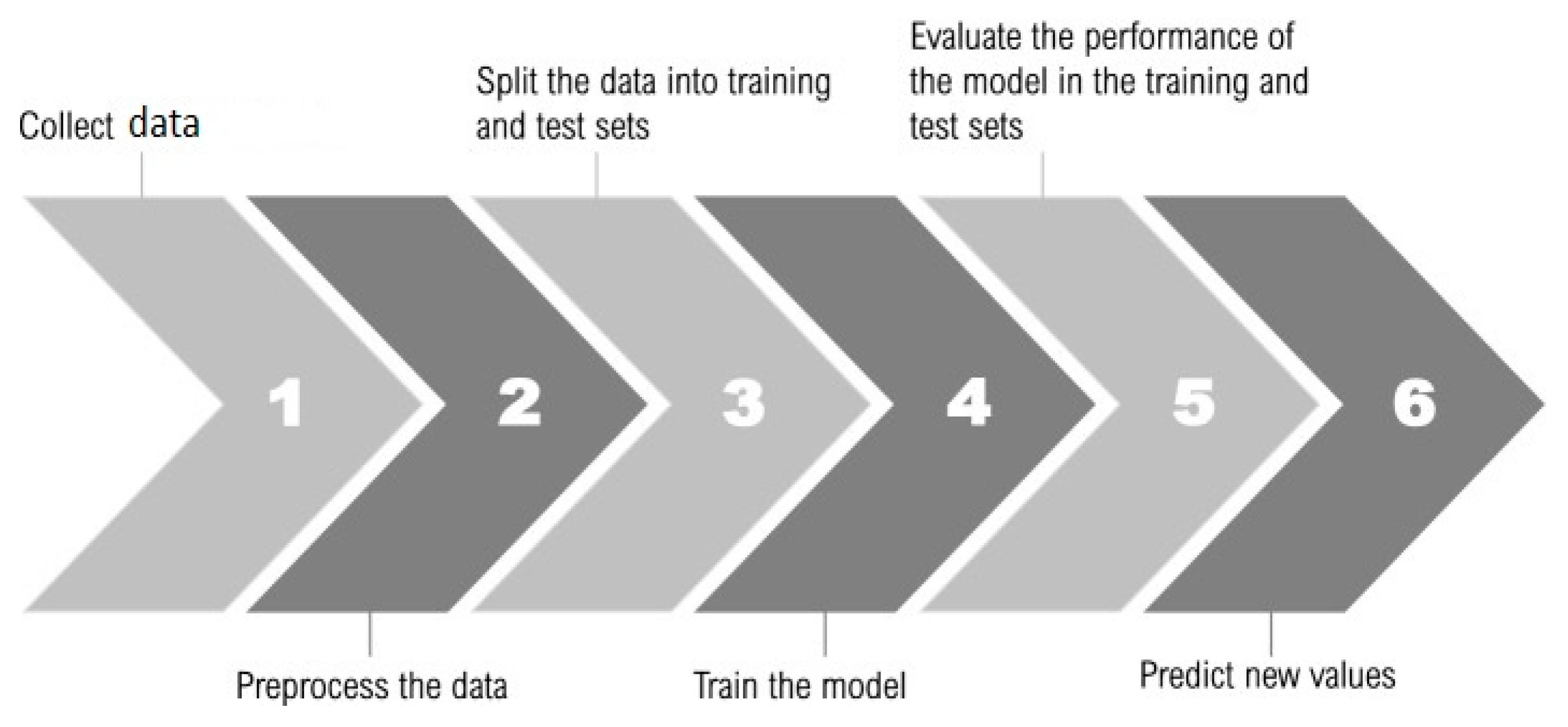
2.5.2. Model Training and Evaluation Strategy

The machine learning component of the SWAT-Prophet-ML framework was trained and evaluated using a train–test split of 80:20, where 80% of the data were used for training and 20% were held out for testing. The dataset consisted of monthly hydrological values for the period 2010–2022, with the Prophet-derived water balance variables (PRECIPmm, PETmm, ETmm, SNOWMELT_PRECIP_ratio) as inputs and the corresponding SWAT-based hydrological response variables (SURQmm, GW_Qmm, SWmm, WYLDmm, SYLDt_ha) as outputs.
To ensure robust model validation, a 5-fold cross-validation was performed on the training set during hyperparameter tuning. Model performance was assessed using RMSE, R2, and Nash–Sutcliffe Efficiency (NSE) across both training and testing sets. Predictions were inverse transformed to their original scale using the MinMaxScaler to allow for direct comparison with actual hydrological outputs.

2.6. Hydrological Scenarios

To assess the reliability and applicability of the predictive modeling framework under varying climatic conditions, this study incorporates two distinct hydrological scenarios: Present Climate Scenario (2010–2022) and Future Climate Scenario (2030–2042). These scenarios were designed to evaluate the model’s ability to simulate hydrological behavior under both observed historical conditions and projected future climate conditions, thereby enhancing the robustness and transferability of the methodology.
Present Climate Scenario (2010–2022): The present scenario uses observed and SWAT-simulated data from 2010 to 2022 as the reference period. This timeframe was selected to capture recent historical variability in climate and hydrological responses, including seasonal and interannual fluctuations in rainfall, snowmelt, ET, PET, surface runoff, groundwater flow, soil water content, water yield, and sediment yield. Data from this period were used to train and validate the SWAT-Prophet-ML model, enabling direct comparison between predicted outputs and established SWAT simulations.
Future Climate Scenario (2030–2042): To quantify the impacts of climate change on watershed hydrology, a future scenario was constructed for the period 2030 to 2042 using SWAT model projections driven by climate data from regional climate models (RCM). These projections incorporated changes in temperature, precipitation, and other meteorological parameters anticipated under Representative Concentration Pathways (RCP). The predicted future values of key hydrological variables were generated using the SWAT-Prophet-ML model, and the outputs were compared with SWAT-projected values to evaluate the model’s capacity to anticipate potential shifts in water availability, runoff patterns, and sediment transport under changing climatic conditions [39].
By employing both present and future scenarios, the study establishes a comparative framework that highlights model performance, prediction accuracy, and sensitivity to climate-induced changes. This approach also allows for the identification of potential vulnerabilities and opportunities in water resource management, enabling stakeholders to make informed decisions based on both current conditions and anticipated future challenges.

3. Results

3.1. SWAT Model Accuracy and Calibration Settings

SWAT was effectively applied to simulate hydrological responses within the Cahaba watershed under varying land use and climatic conditions. The model was initially configured using the 2011 land use/land cover and 1980–2010 and 2010–2040 climate data across eight sub-basins, 15 land-use classes, and 30 soil categories. It was later calibrated using 2011 LULC under the same climate conditions. Hydrologic calibration and validation were conducted at the Trussville station in the upper Cahaba watershed. During calibration, wet conditions prevailed, and major peak flows observed in late March and early April were attributed to late snowmelt and spring runoff. The model demonstrated reasonable accuracy, achieving NSE and R2 values of 0.565 and 0.591 respectively. The coefficient of determination (R2) improved from 0.542 during calibration to 0.591 during validation, potentially due to the dominance of low streamflow events in the validation period, which reduced variability and increased correlation (Table 3). Key parameters such as ESCO (Soil Evaporation Compensation Factor) and CN2 (SCS Curve Number) were identified as highly sensitive to streamflow under wet conditions. Nutrient-related parameters (N_UPDIS, P_UPDIS) and urban erosion indicators (RILL_MULT, C_FACTOR) also showed significant influence on model outputs.

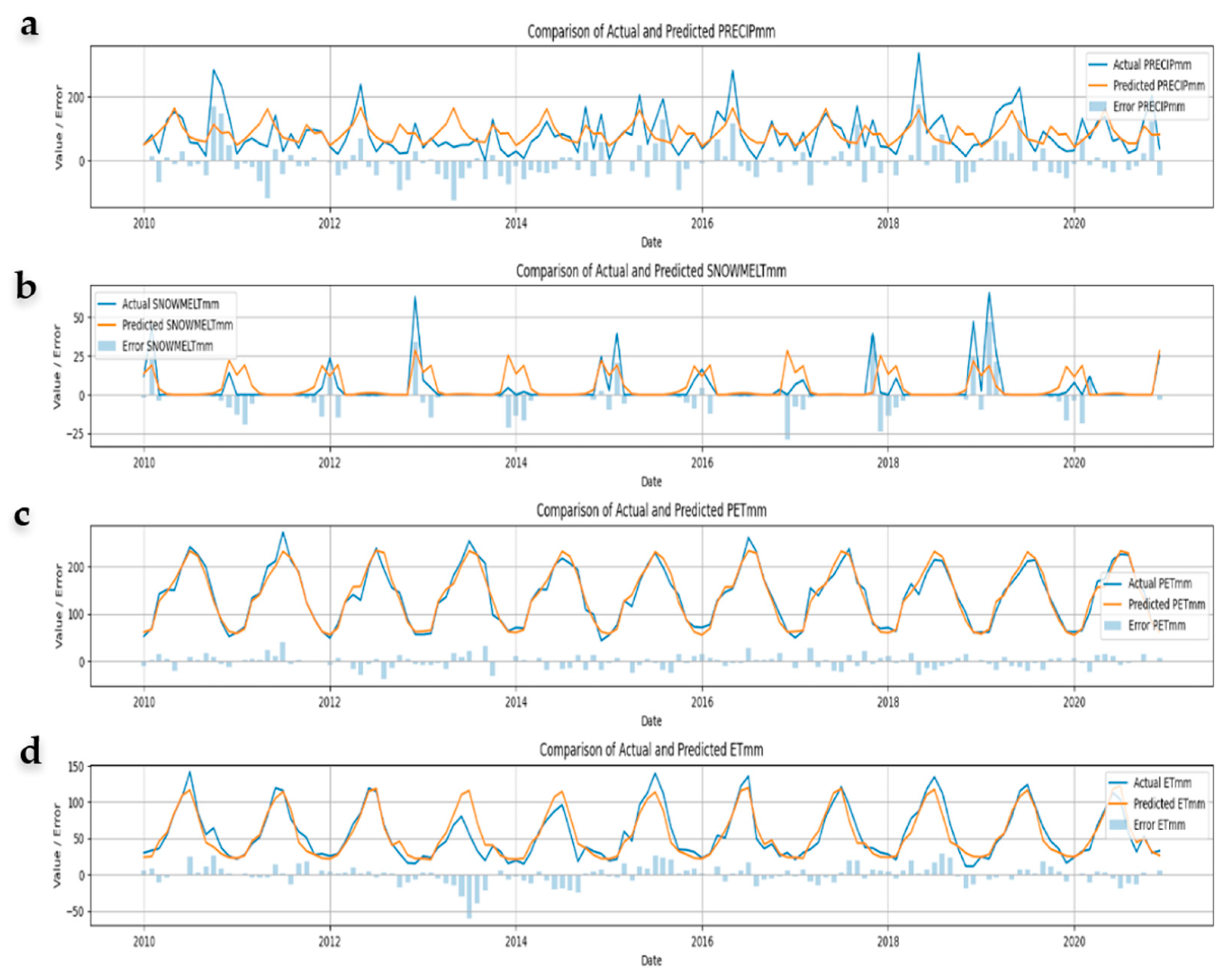
3.2. SWAT vs. SWAT-Prophet-ML for Water Balance Predictions in Present Climate

Historical trends in environmental variables such as ET, PET, precipitation, and snowmelt show distinct seasonal patterns (Figure 4). Actual measurements reveal cyclic fluctuations, likely influenced by climatic factors such as temperature, precipitation cycles, and snow accumulation. For the present climate between 2010 and 2022, the predicted values from the SWAT-Prophet-ML model appear to align closely with actual data from the SWAT model for ET and PET but show noticeable deviations for more variable phenomena like precipitation and snowmelt. The current analysis demonstrates progress in modeling these environmental variables, with prediction errors of RMSE for ET, PET, precipitation, and snowmelt as 15 mm–20 mm, 10 mm–15 mm, 30 mm–50 mm, and 5 mm–10 mm, respectively.
For variables with higher variability such as precipitation, and snowmelt, the SWAT-Prophet-ML model struggles to capture extreme events accurately, evident in spikes and dips in error trends. This shows that SWAT-Prophet-ML is likely well suited for smooth and periodic patterns, but less reliable for extreme or abrupt hydrological changes for present climate conditions. Continued refinement of these models can lead to better forecasting, aiding in applications like agricultural planning, water resource management, and climate monitoring. Improved prediction accuracy will likely emerge from integrating higher-resolution climatic data, advanced machine learning algorithms, and better representation of feedback loops in the models [40]. Future work can also focus on reducing errors during extreme weather conditions to enhance the model’s robustness. The performance of the SWAT-Prophet-ML model in predicting the four variables that directly or indirectly affect water balance in the watershed for the present climate is provided in Table 4.

Limitations in Capturing Peak Events

While the Prophet model effectively decomposes time series into trend and seasonal components, it exhibits notable limitations in capturing sharp, short-duration peak events, such as heavy rainfall spikes or sudden snowmelt. This is largely due to Prophet’s underlying additive model structure, which assumes smooth and regular seasonal patterns. As a result, it tends to smooth over localized outliers, treating them as noise rather than meaningful extremes. Furthermore, Prophet assumes piecewise linear or logistic growth for the trend component and may fail to adapt to abrupt shifts or high-frequency variability unless such events are consistently present in the historical data. In the context of hydrological forecasting, this behavior limits the model’s ability to anticipate critical extreme events that significantly influence surface runoff, flash flooding, or sediment transport. For instance, as shown in Figure 4b,c, Prophet underestimates peak values during storm months, leading to under-propagation of signal amplitude into downstream ML predictions. Future model improvements will consider integrating spike-aware models, such as quantile regression or hybrid Prophet-LSTM structures, and incorporating event-based decomposition techniques to better preserve and forecast peak behaviors.

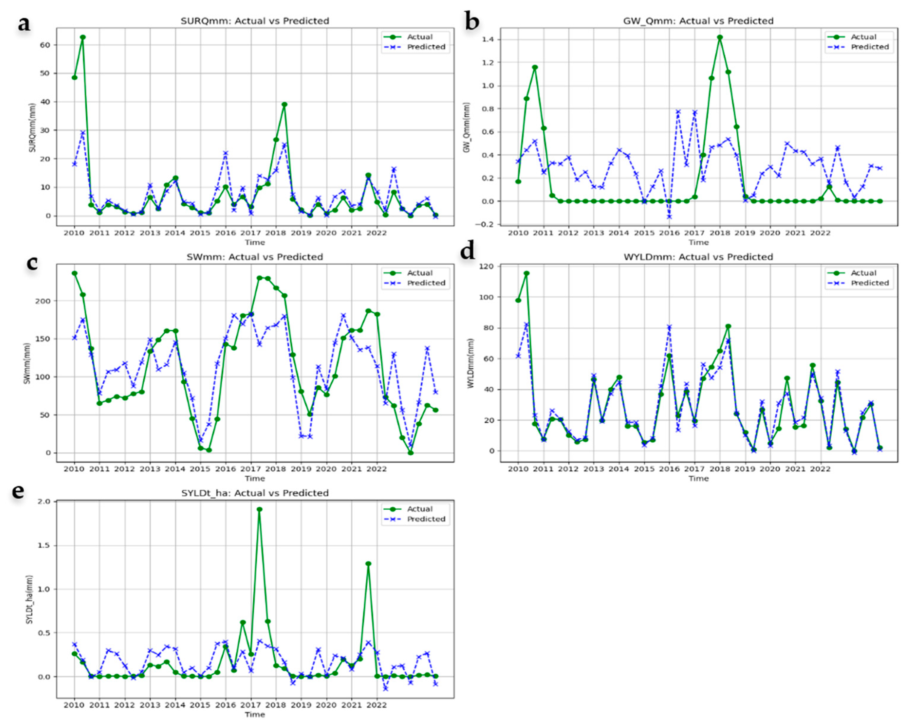
3.3. SWAT vs. SWAT-Prophet-ML for Hydrological Response Predictions in Present Climate

The graphs illustrate historical data trends for various hydrological responses in the Cahaba watershed based on SWAT and SWAT-Prophet-ML model predictions (Figure 5). The X-axis in Figure 5 denotes the periodic time between 2010 and 2022 scaled as 0 to 40. In the present climate, the SWAT model estimates pointed to specific spikes and fluctuations that likely correspond to extreme hydrological events [41,42]. The groundwater contribution to streamflow shows pronounced peaks for 2011 (1.21 mm) and 2019 (1.45 mm) based on SWAT estimates, indicating substantial groundwater flow during those periods. However, the novel SWAT-Prophet-ML model underpredicted the groundwater contribution to streamflow values as 0.53 mm for 2011 and 0.61 mm for 2019. Overall, it can be stated that for the groundwater contribution to streamflow and sediment yields, the novel model struggles to capture extreme peaks precisely, though it performs reasonably well for baseline conditions [43].
The predictions of the surface runoff contribution to streamflow and water yields in both models are in good correlation, with coefficient of determination R2 values of 0.65 and 0.75, respectively. They also highlight significant runoff and water yield patterns in response to extreme precipitation events for the years 2011 and 2019 (Figure 4). These historical patterns have been instrumental in understanding seasonal variations and system responses [44]. This comparison highlights areas where the prediction model aligns closely with observed data and areas where it deviates, offering critical insights into the model’s strengths and limitations. The wave patterns in the soil water content are captured well by the SWAT-Prophet-ML model while there is possible underestimation in higher soil moisture zones relative to the SWAT model [45]. The performance of the SWAT-Prophet-ML model in predicting the five hydrological responses for the present climate is provided in Table 5. Even though there are limitations of RMSE, R2, and NSE in capturing extreme hydrological events, these metrics are widely accepted in hydrological modeling for evaluating overall model performance across different flow conditions [46]. Our study focuses on simulating continuous streamflow, not exclusively extreme events, making these metrics appropriate for establishing baseline performance. The evaluation period includes extreme years like 2011 and 2019, so the metrics still reflect model behavior under such conditions.
Moving forward, there is significant potential to enhance prediction accuracy through several approaches. Incorporating additional variables, such as soil moisture, temperature, and land use, may refine model predictions. Exploring advanced machine learning techniques, such as ensemble models or neural networks, could better capture nonlinear relationships evident in the data. Developing predictive scenarios for varying climate and land-use conditions will improve preparedness for future events [47].

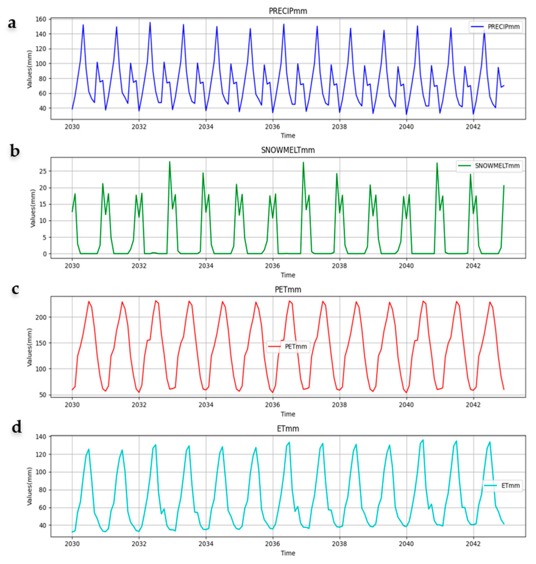
3.4. SWAT-Prophet-ML-Based Water Balance Predictions in Future Climate

From 2030 to 2042, projections of the four water balance components show strong seasonal trends using the SWAT-Prophet-ML model (Figure 6). ET and PET maintain smooth, consistent annual cycles, indicating high model reliability for temperature-driven processes. PET consistently exceeds ET by 50–65%, aligning with theoretical expectations as per the novel model outcomes. In future climate, precipitation ranging between 20 mm and 150 mm and snowmelt ranging between 0 mm and 29 mm exhibit more variability, with sharp peaks suggesting possible extreme weather events. Despite this, both retain regular annual patterns, reflecting the model’s strength in capturing seasonality. The SWAT-Prophet-ML modeling results show that the future climate predictions of precipitation (20 mm–150 mm) are decreasing relative to the present climate estimates of precipitation (40 mm–165 mm), whereas the future climate predictions of snowmelt (0 mm–29 mm) are increasing relative to the present climate estimates of snowmelt (0 mm–26 mm). This indicates that rainfall is likely to decrease in future with increases in snow melting and soil water accumulation [48]. These patterns suggest stable climatic behavior over the projection period, though the seasonal fluctuations highlight areas for model refinement for the SWAT-Prophet-ML model [49]. Continued improvements, especially in simulating precipitation and snowmelt extremes, will enhance forecasting accuracy. These projections support long-term planning in water resource management, agriculture, and climate resilience. Incorporating higher-resolution data and improving model responsiveness to extreme events will be essential for strengthening predictive capabilities in future climate modeling efforts.

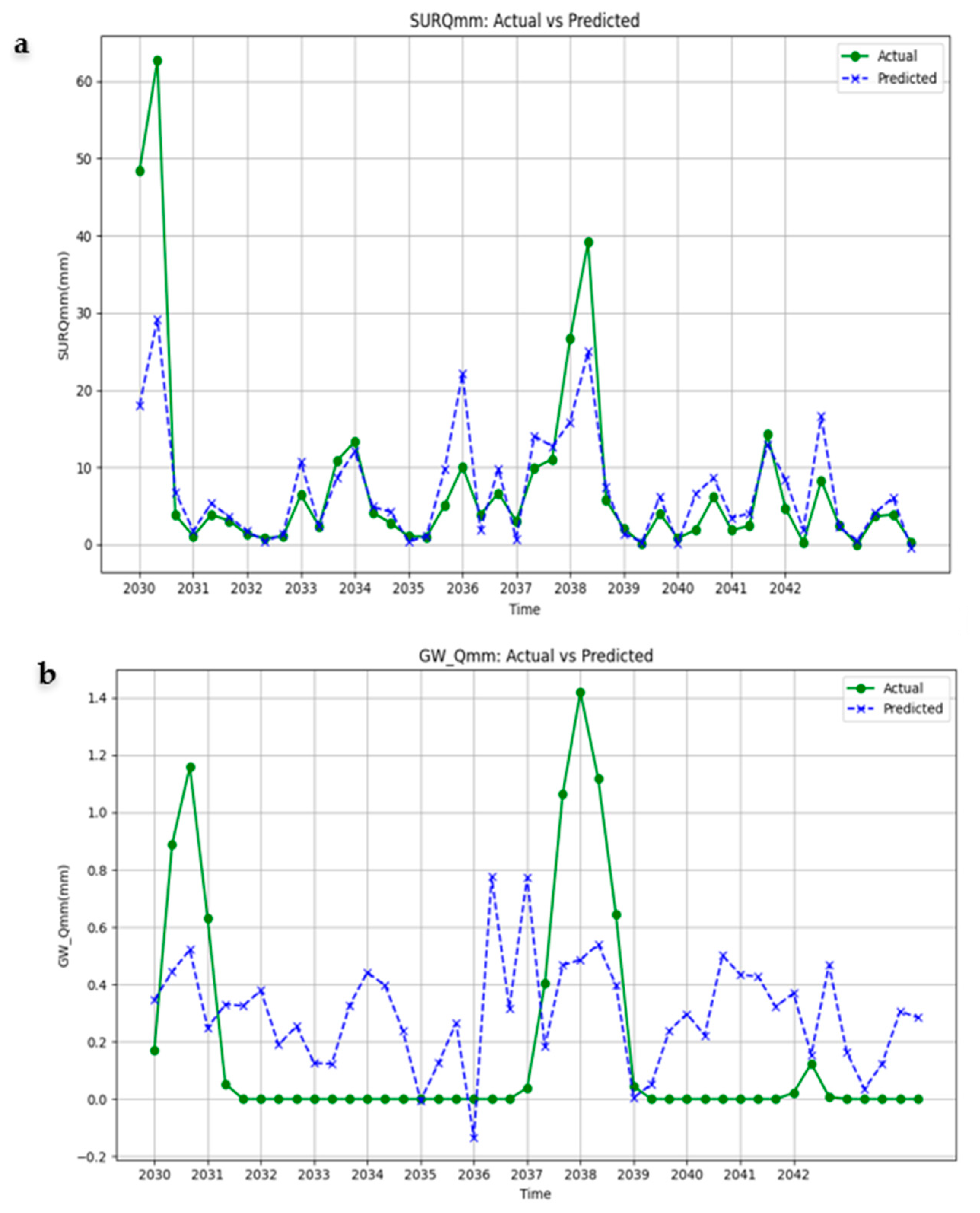
3.5. SWAT vs. SWAT-Prophet-ML for Hydrological Response Predictions in Future Climate

The graphs compare the future climatic trends for two hydrological responses in the Cahaba watershed based on SWAT and SWAT-Prophet-ML model predictions (Figure 7). The X-axis in Figure 7 denotes the periodic time between 2030 and 2042 scaled as 0 to 40. The results evaluate whether the data-driven novel model can replicate or approximate the physically based outputs of the SWAT model for the key hydrologic responses under projected future conditions. The core objective of this comparison was to evaluate the predictive capacity of a machine learning-driven framework when used alongside traditional physically based models to simulate hydrological processes under non-stationary climate conditions [50,51]. While the SWAT-Prophet-ML model, trained on SWAT’s historical inputs and outputs, was able to replicate baseline hydrological trends with reasonable accuracy under current climate scenarios, it failed to generate reliable outputs for future climate projections [52]. This is evident in the divergence of predicted trends for the surface and groundwater contributions when compared to the SWAT model under projected climate data.

3.5.1. Limitations of the SWAT-Prophet-ML Model in Future Climate

Machine learning models like Prophet rely on patterns and trends in historical data but lack an explicit understanding of physical processes. They cannot inherently simulate critical hydrologic processes such as infiltration, evapotranspiration, baseflow, or groundwater recharge especially when the system operates under new climatic regimes which are not reflected in historical training data [53]. In this study, the novel model was trained on SWAT outputs calibrated for present climate conditions. Hence, the Prophet-ML component likely overfitted to stationary trends, reducing its ability to generalize to unseen future inputs where precipitation and temperature patterns deviate significantly. Additionally, the Cahaba watershed exhibits complex semi-distributed hydrological behavior governed by nonlinear interactions between land use, soil properties, topography, and climate. These interactions are well captured in SWAT’s conceptual process-based structure but are simplified in the time-series-based Prophet-ML model [54]. Future climate conditions represent out-of-distribution data for the ML model, which was not explicitly trained on climate-perturbed datasets. This makes the model poorly equipped to adapt to changes in rainfall intensity, frequency, or seasonal shifts that significantly alter the water balance. However, techniques such as detailed hyperparameter optimization are beyond the scope of the current study, which focuses primarily on evaluating the hydrological impacts under different climate scenarios using established model configurations.
To enhance the performance of hybrid hydrological models under changing climate scenarios, ML models could be used beneficially for data fusion rather than directly replacing them for physical hydrological modeling [55]. Another technique could be to train ML models on a wider range of scenario-based data, including climate inputs from multiple global and regional climate change scenarios to improve generalization under non-stationary conditions. As the SWAT model works on the basic principle of water balance, it will be effective to incorporate mass balance functions during ML and Prophet predictions [56,57]. Performing input sensitivity analysis to understand which meteorological or hydrological variables most affect model performance, and target those in model refinement is also recommended.

3.6. Performance Evaluation of Various Modeling Techniques in Present Climate

The performance evaluation yielded the following results for present climate predictions in the Cahaba watershed as described in Table 6.
Code 1: Achieved the highest performance score of 86.73%, emphasizing a well-rounded machine learning workflow and justified by its use of a comprehensive systematic framework of the SWAT-Prophet-ML model.
Code 2: Received a performance rating of 85%, with the use of the SWAT model, emphasizing a well-calibrated hydrological modeling process.
Code 3: Scored 81.25%, attributed to its ability to train and forecast future values, and its use of statistical metrics for evaluation, suggesting a focus on predictive accuracy with the use of the SWAT-Prophet model.

Evaluation Methodology and Use of SWAT as Reference

The performance evaluation results in Section 3.6 (Codes 1–3) were derived from a comparative analysis of three modeling configurations applied to the Cahaba watershed under present climate conditions (2010–2022). These configurations include: (1) the proposed SWAT-Prophet-ML model, (2) the baseline SWAT model, and (3) the intermediate SWAT-Prophet model. Model accuracy was assessed using a set of evaluation metrics including RMSE, R2, and NSE, applied to both water balance components and hydrological response variables.
To ensure consistency in comparison, each model was run over the same input time series, and the SWAT model outputs were used as the reference or “actual” values when calculating the error metrics for the Prophet-based and ML-based models. This approach was taken for the following reasons:
  • Lack of continuous, high-resolution observational data: Field-measured observational data for all required hydrological components (e.g., groundwater contribution, soil moisture, sediment yield) were not available at finer spatial and temporal resolution for the entire watershed.
  • The SWAT model was previously calibrated and validated using available observed data (streamflow, surface runoff) for the Cahaba River Basin). Its outputs are, therefore, treated as a reliable physical baseline to evaluate enhancements from additional forecasting layers.
  • This modeling chain focuses on enhancing SWAT forecasts through decomposition (Prophet) and regression (ML), not replacing SWAT. Hence, performance is measured relative to the benchmark simulation rather than raw observations.
The performance percentages reported in Table 6 represent a normalized aggregation of metric values across all predicted variables, where higher scores indicate better overall fidelity to SWAT’s baseline estimates. Although SWAT is not a direct substitute for observational truth, its physically based structure provides a stable, interpretable reference for model validation in data-sparse hydrological settings.

4. Discussion and Future Work

4.1. Enhancing Model Generalization Under Future Climate Regimes

The reduced performance of the SWAT-Prophet-ML framework under future climate scenarios, as discussed in Section 3.5.1, is primarily due to the model’s reliance on historical data distributions, which do not reflect the increased variability, shifts in precipitation patterns, and altered temperature regimes expected in future conditions. Prophet and polynomial regression are fundamentally trained on stationary trends, making them vulnerable to failure under non-stationary, out-of-distribution inputs.
To address this, we propose several enhancements to improve generalization under future conditions:
  • Scenario-Based Synthetic Training: Future iterations of this model will incorporate SWAT-generated outputs under multiple Representative Concentration Pathway (RCP) scenarios as training inputs, expanding the model’s exposure to a broader range of climatic conditions.
  • Data Augmentation: We plan to generate perturbed versions of climate input variables (e.g., rainfall intensity shifts, temperature anomalies) using Gaussian noise or bootstrapping methods to improve robustness to rare or extreme events.
  • Physically Informed Constraints: Incorporating mass balance principles directly into the loss function or model architecture (e.g., conservation-aware ML or physics-guided neural networks) will ensure hydrologic plausibility, even when data distributions deviate from historical norms.
  • Transfer Learning Techniques: Pretraining models on global climate-simulated datasets and fine-tuning on watershed-specific data could improve adaptability to novel climate regimes, especially in data-scarce basins.
These directions will not only strengthen the model’s applicability to changing climate scenarios but also improve its scalability for deployment in diverse hydrological settings globally.

4.2. Comparative Evaluation with Ensemble and Deep Learning Models

While this study establishes the feasibility and accuracy of the SWAT-Prophet-ML framework using multi-output regression with polynomial features, future work will expand the modeling pipeline to include state-of-the-art ensemble and deep learning models such as Random Forest (RF), Gradient Boosting Machines (GBM), and Long Short-Term Memory (LSTM) networks. These models have been extensively validated in hydrology for their ability to capture high-dimensional nonlinear relationships and temporal dependencies [10,38]. Comparative performance evaluation will be conducted using cross-validated RMSE, NSE, and R2 metrics, and statistical significance of performance differences will be assessed using paired tests. Importantly, to address model interpretability, a limitation in many black-box models, we will employ SHAP (SHapley Additive exPlanations) for tree-based models and attention-based visualizations for LSTM models to quantify feature influence on individual predictions. This approach aims to provide both predictive strength and domain interpretability, which are critical for informing climate-resilient water policy decisions. By benchmarking the existing polynomial model against these alternatives, we aim to validate the robustness of our proposed hybrid structure and identify cases where more advanced architectures yield substantial benefit over simpler regression approaches.

4.3. Uncertainty in Prophet Forecasts and Practical Implications

The Prophet model inherently produces uncertainty estimates via 95% prediction intervals (PIs), which account for variability in the trend, seasonality, and model residuals. These intervals are especially useful for communicating the reliability of forecasts in real-world water resource management scenarios. In this study, prediction intervals were generated alongside point forecasts for key water balance variables, including precipitation, ET, PET, and snowmelt, across both present and future climate scenarios.
While the intervals offer valuable information about forecast spread and model confidence, several limitations affect their practical interpretability:
  • Under present climate conditions, Prophet’s uncertainty remains relatively narrow for smooth variables like ET and PET, enhancing confidence in monthly water demand and planning decisions.
  • However, for highly variable phenomena such as precipitation and snowmelt, especially under future climate projections (2030–2042), the uncertainty intervals widen substantially. This reflects not only inherent input variability but also the model’s inability to anticipate regime shifts or outliers outside the historical data distribution.
  • Because the downstream ML model in the SWAT-Prophet-ML pipeline depends on Prophet outputs, errors or overconfident predictions from Prophet may propagate, potentially affecting the reliability of surface runoff, water yield, or sediment yield predictions.
From a practical standpoint, these wide uncertainty intervals reduce the confidence of hydrologists and decision-makers in using model outputs for fine-grained policy recommendations, especially for extreme event forecasting. For example, large uncertainty in precipitation forecasts may hinder reservoir operations or flood mitigation planning.
To address these issues, future work will include:
  • Quantile regression forests or Bayesian models to generate more robust uncertainty estimates.
  • Calibration of Prophet’s uncertainty intervals using historical residual validation.
  • Monte Carlo dropout or ensemble-based simulations to propagate uncertainty through the full pipeline (SWAT → Prophet → ML).
  • Expressing results not just as deterministic outputs but as probabilistic forecasts that better support risk-informed decision-making.

5. Conclusions

This study proposed a hybrid modeling framework, SWAT-Prophet-ML, that integrates physically based hydrological simulation (SWAT), time-series decomposition (Prophet), and machine learning (multi-output polynomial regression) to forecast monthly water balance and hydrological response variables in the climate-sensitive Cahaba watershed.
Key Findings: Present Climate Scenario (2010–2022)
  • Model demonstrated strong predictive performance for water yield (R2 = 0.75), surface runoff (R2 = 0.70), evapotranspiration and potential evapotranspiration (RMSE = 15–20 mm)
  • Accurate modeling of seasonal trends and smooth climatic behavior was achieved using the Prophet-decomposed features.
  • Precipitation and snowmelt showed higher variability and were less accurately predicted (RMSE = 30–50 mm and 5–10 mm, respectively).
Key Findings: Future Climate Scenario (2030–2042)
  • Model underperformed, especially for variables like groundwater flow and sediment yield, where the hybrid model failed to capture peak years or sharp shifts.
  • The main cause was the model’s reliance on stationary historical patterns, which are not representative of future climate variability.
Model Limitations:
  • Lack of training on non-stationary or perturbed climate data
  • Absence of physical constraints in ML predictions
  • Limited capacity to simulate extreme events or abrupt hydrological shifts
Future Work Directions:
  • Scenario-based training using synthetic climate inputs from multiple representative concentration pathways
  • Data augmentation techniques to simulate rare or extreme meteorological conditions
  • Physically informed modeling, integrating hydrological constraints into the ML component
  • Model benchmarking using ensemble and deep learning with SHAP-based feature interpretation
This study provides a modular, semi-automated framework that bridges physical hydrological modeling and data-driven forecasting. While highly effective under historical climate conditions, it also highlights the importance of generalization strategies for adapting predictive models to future climate regimes. The work contributes a replicable architecture for modern hydrological forecasting and offers a roadmap for advancing climate-resilient water resource management.

Author Contributions

Conceptualization, methodology, data curation, and writing—S.K.D.; Conceptualization, methodology, and writing—P.P.; conceptualization, review, and editing—H.M.G. All authors have read and agreed to the published version of the manuscript.

Funding

This work was partially funded by a research grant awarded by the National Science Foundation: NSF EPSCOR Track-2 grant (OIA RII Track2 Award no. 2019561): IGM—A Framework for Harnessing Big Hydrological Datasets for Integrated Groundwater Management, and MIT Lincoln Laboratory Climate Initiative support under the Department of the Air Force Contract No. FA8702-15-D-0001. Any opinions, findings, conclusions or recommendations expressed in this material are those of the authors and do not necessarily reflect the views of the Department of the Air Force.

Data Availability Statement

The data presented in this study are available on request from the corresponding author due to the ongoing and additive testing nature of the research about using time-series models in hydrological applications.

Acknowledgments

We would like to acknowledge the reviewers for enhancing the article.

Conflicts of Interest

Hari Manikanta Ghantasala is from Moschip Technologies Pvt Ltd. The authors declare that they have no conflicts of interests that could have appeared to influence the work reported in this paper.

References

  1. Kode, V.R.; Preetha, P.; Kodali, D. Chapter 26—Smart boron nitride nanomaterial systems for wastewater treatment studies. In Micro and Nano Technologies, Smart Nanomaterials for Environmental Applications; Ayeleru, O.O., Idris, A.O., Pandey, S., Olubambi, P.A., Eds.; Elsevier: Amsterdam, The Netherlands, 2025; pp. 649–676. ISBN 9780443217944. [Google Scholar] [CrossRef]
  2. Li, Z.; Zhang, Y.; Wang, Z. Hydrological modeling using remote sensing and machine learning. J. Hydrol. 2019, 572, 678–689. [Google Scholar]
  3. Xu, Y.; Gao, Y.; Zhang, D. Evaluation of evapotranspiration estimation methods under climate variability. J. Hydrol. 2021, 599, 126414. [Google Scholar]
  4. Allen, R.G.; Pereira, L.S.; Raes, D.; Smith, M. Crop Evapotranspiration: Guidelines for Computing Crop Water Requirements. FAO 1998, 300, D05109. [Google Scholar]
  5. Salas, J.D.; Delleur, J.W.; Yevjevich, V.; Lane, W.L. Applied Modeling of Hydrologic Time Series; Water Resources Publications: Highlands Ranch, CO, USA, 2012. [Google Scholar]
  6. Taylor, S.J.; Letham, B. Forecasting at scale. Am. Stat. 2018, 72, 37–45. [Google Scholar] [CrossRef]
  7. Singh, A.; Jain, S.K.; Tyagi, B. Rainfall forecasting using Prophet model. Hydrol. Sci. J. 2020, 65, 716–726. [Google Scholar]
  8. Zubair, M.; Rehman, S. Time-series forecasting of climate variables using Prophet model. Clim. Dyn. 2022, 59, 123–135. [Google Scholar]
  9. Solomatine, D.; Ostfeld, A. Data-driven modeling: Some past experiences and new approaches. J. Hydroinforma. 2008, 10, 3–22. [Google Scholar] [CrossRef]
  10. Mosavi, A.; Ozturk, P.; Chau, K.W. Flood prediction using machine learning models. Sustainability 2018, 10, 4206. [Google Scholar]
  11. Preetha, P.P.; Joseph, N.; Narasimhan, B. Quantifying surface water and ground water interactions using a coupled SWAT_FEM model: Implications of management practices on hydrological processes in irrigated river basins. Water Resour. Manag. 2021, 35, 2781–2797. [Google Scholar] [CrossRef]
  12. Gonzalez, M.O.; Preetha, P.; Kumar, M.; Clement, T.P. Comparison of data-driven groundwater recharge estimates with a process-based model for a river basin in the southeastern USA. J. Hydrol. Eng. 2023, 28, 04023019. [Google Scholar] [CrossRef]
  13. Preetha, P.; Al-Hamdan, A. A union of dynamic hydrological modeling and satellite remotely-sensed data for spatiotemporal assessment of sediment yields. Remote Sens. 2022, 14, 400. [Google Scholar] [CrossRef]
  14. Wang, Z.G.; Liu, C.M.; Wu, X.F. A review of the studies on distributed hydrological model based on DEM. J. Nat. Resour. 2003, 18, 168–173. [Google Scholar]
  15. Ahmad, S.; Kalra, A.; Stephen, H. Estimating soil moisture using remote sensing data: A machine learning approach. Adv. Water Resour. Res. 2010, 33, 69–80. [Google Scholar] [CrossRef]
  16. Preetha, P.P.; Al-Hamdan, A.Z. Synergy of remotely sensed data in spatiotemporal dynamic modeling of the crop and cover management factor. Pedosphere 2022, 32, 381–392. [Google Scholar] [CrossRef]
  17. Preetha, P.P.; Maclin, K. Evaluation of Hydrogeological Models and Big Data for Quantifying Groundwater Use in Regional River Systems. In Environmental Processes and Management: Tools and Practices for Groundwater; Springer International Publishing: Cham, Switzerland, 2023; pp. 189–206. [Google Scholar]
  18. Moriasi, D.N.; Arnold, J.G.; Van Liew, M.W.; Bingner, R.L.; Harmel, R.D.; Veith, T.L. Veith Model Evaluation Guidelines for Systematic Quantification of Accuracy in Watershed Simulations. Trans. ASABE 2007, 50, 885–900. [Google Scholar] [CrossRef]
  19. Brown, C. Decision scaling for robust planning and policy under climate uncertainty. Water Resour. Res. 2013, 49, 3418–3432. [Google Scholar]
  20. Wang, S.; Huang, G.H.; Baetz, B.W.; Huang, W. A polynomial chaos ensemble hydrologic prediction system for efficient parameter inference and robust uncertainty assessment. J. Hydrol. 2015, 530, 716–733. [Google Scholar] [CrossRef]
  21. Preetha, P.P.; Al-Hamdan, A.Z.; Anderson, M.D. Assessment of climate variability and short-term land use land cover change effects on water quality of Cahaba River Basin. Int. J. Hydrol. Sci. Technol. 2021, 11, 54–75. [Google Scholar] [CrossRef]
  22. Preetha, P.; Hasan, M. Scrutinizing the Hydrological Responses of Chennai, India Using Coupled SWAT-FEM Model under Land Use Land Cover and Climate Change Scenarios. Land 2023, 12, 938. [Google Scholar] [CrossRef]
  23. Lange, H.; Sippel, S. Machine learning applications in hydrology. In Forest-Water Interactions; Springer International Publishing: Cham, Switzerland, 2020; pp. 233–257. [Google Scholar]
  24. Zounemat-Kermani, M.; Batelaan, O.; Fadaee, M.; Hinkelmann, R. Ensemble machine learning paradigms in hydrology: A review. J. Hydrol. 2021, 598, 126266. [Google Scholar] [CrossRef]
  25. Rujoiu-Mare, M.; Mihai, B. Mapping land cover using remote sensing data and GIS techniques: A case study of Prahova Subcarpathians. Procedia Environ. Sci. 2016, 32, 244–255. [Google Scholar] [CrossRef]
  26. Dechmi, F.; Burguete, J.; Skhiri, A. SWAT application in intensive irrigation systems: Model modification, calibration and validation. J. Hydrol. 2012, 470, 227–238. [Google Scholar] [CrossRef]
  27. Graves, P.H.; Ward, G.M. Mayfly and stonefly distribution in the mainstem Cahaba River, Alabama. Southeast. Nat. 2011, 10, 477–488. [Google Scholar] [CrossRef]
  28. Lekkala, C. Bridging the Gap: Evaluating Traditional, Hybrid (Prophet), and Deep Learning Approaches in Time Series Forecasting. J. Artif. Intell. Mach. Learn. Data Sci. 2024, 2, 933–937. [Google Scholar] [CrossRef]
  29. Rahman, A.T.M.S.; Hosono, T.; Kisi, O.; Dennis, B.; Imon, A.H.M.R. A minimalistic approach for evapotranspiration estimation using the Prophet model. Hydrol. Sci. J. 2020, 65, 1994–2006. [Google Scholar] [CrossRef]
  30. Xu, T.; Liang, F. Machine learning for hydrologic sciences: An introductory overview. Wiley Interdiscip. Rev. Water 2021, 8, e1533. [Google Scholar] [CrossRef]
  31. Cappelli, F.; Grimaldi, S. Feature importance measures for hydrological applications: Insights from a virtual experiment. Stoch. Environ. Res. Risk Assess. 2023, 37, 4921–4939. [Google Scholar] [CrossRef]
  32. Ichiba, A.; Gires, A.; Tchiguirinskaia, I.; Schertzer, D.; Bompard, P.; Ten Veldhuis, M.-C. Scale effect challenges in urban hydrology highlighted with a distributed hydrological model. Hydrol. Earth Syst. Sci. 2018, 22, 331–350. [Google Scholar] [CrossRef]
  33. Wang, S.; Peng, H.; Hu, Q.; Jiang, M. Analysis of runoff generation driving factors based on hydrological model and interpretable machine learning method. J. Hydrol. Reg. Stud. 2022, 42, 101139. [Google Scholar] [CrossRef]
  34. Díaz-González, L.; Uscanga-Junco, O.A.; Rosales-Rivera, M. Development and comparison of machine learning models for water multidimensional classification. J. Hydrol. 2021, 598, 126234. [Google Scholar] [CrossRef]
  35. Preetha, P.P.; Al-Hamdan, A.Z. Multi-level pedotransfer modification functions of the USLE-K factor for annual soil erodibility estimation of mixed landscapes. Model. Earth Syst. Environ. 2019, 5, 767–779. [Google Scholar] [CrossRef]
  36. Safari, M.J.S.; Arashloo, S.R.; Vaheddoost, B. Fast multi-output relevance vector regression for joint groundwater and lake water depth modeling. Environ. Model. Softw. 2022, 154, 105425. [Google Scholar] [CrossRef]
  37. Ghorbanidehno, H.; Kokkinaki, A.; Lee, J.; Darve, E. Recent developments in fast and scalable inverse modeling and data assimilation methods in hydrology. J. Hydrol. 2020, 591, 125266. [Google Scholar] [CrossRef]
  38. Ji, H.; Chen, Y.; Fang, G.; Li, Z.; Duan, W.; Zhang, Q. Adaptability of machine learning methods and hydrological models to discharge simulations in data-sparse glaciated watersheds. J. Arid. Land 2021, 13, 549–567. [Google Scholar] [CrossRef]
  39. NOAA. Average Temperature: Stabilized Emissions, Projections. Climate.Gov. 2017. Available online: https://www.noaa.gov/climate (accessed on 4 October 2017).
  40. Mosaffa, H.; Sadeghi, M.; Mallakpour, I.; Jahromi, M.N.; Pourghasemi, H.R. Application of machine learning algorithms in hydrology. In Computers in Earth and Environmental Sciences; Elsevier: Amsterdam, The Netherlands, 2022; pp. 585–591. [Google Scholar]
  41. Preetha, P.P.; Al-Hamdan, A.Z. Developing nitrate-nitrogen transport models using remotely-sensed geospatial data of soil moisture profiles and wet depositions. J. Environ. Sci. Health A 2020, 55, 615–628. [Google Scholar] [CrossRef]
  42. Preetha, P.P.; Al-Hamdan, A.Z. Integrating finite-element-model and remote-sensing data into SWAT to estimate transit times of nitrate in groundwater. Hydrogeol. J. 2020, 28, 2187–2205. [Google Scholar] [CrossRef]
  43. Petty, T.R.; Dhingra, P. Streamflow hydrology estimate using machine learning (SHEM). JAWRA J. Am. Water Resour. Assoc. 2018, 54, 55–68. [Google Scholar] [CrossRef]
  44. Preetha, P.; Joseph, N. Evaluating Modified Soil Erodibility Factors with the Aid of Pedotransfer Functions and Dynamic Remote-Sensing Data for Soil Health Management. Land 2025, 14, 657. [Google Scholar] [CrossRef]
  45. Wankmüller, F.J.P.; Delval, L.; Lehmann, P.; Baur, M.J.; Cecere, A.; Wolf, S.; Or, D.; Javaux, M.; Carminati, A. Global influence of soil texture on ecosystem water limitation. Nature 2024, 635, 631–638. [Google Scholar] [CrossRef]
  46. Rozos, E.; Dimitriadis, P.; Bellos, V. Machine learning in assessing the performance of hydrological models. Hydrology 2021, 9, 5. [Google Scholar] [CrossRef]
  47. Preetha, P.; Bathi, J.R.; Kumar, M.; Kode, V.R. Predictive Tools and Advances in Sustainable Water Resources Through Atmospheric Water Generation Under Changing Climate: A Review. Sustainability 2025, 17, 1462. [Google Scholar] [CrossRef]
  48. Labat, D.; Goddéris, Y.; Probst, J.L.; Guyot, J.L. Evidence for global runoff increase related to climate warming. Adv. Water Resour. 2004, 27, 631–642. [Google Scholar] [CrossRef]
  49. Tandon, A.; Awasthi, A.; Pattnayak, K.C. Efficacy of machine learning in simulating precipitation and its extremes over the capital cities in North Indian states. Sci. Rep. 2025, 15, 10345. [Google Scholar] [CrossRef]
  50. Yang, T.; Sun, F.; Gentine, P.; Liu, W.; Wang, H.; Yin, J.; Du, M.; Liu, C. Evaluation and machine learning improvement of global hydrological model-based flood simulations. Environ. Res. Lett. 2019, 14, 114027. [Google Scholar] [CrossRef]
  51. Shen, C.; Chen, X.; Laloy, E. Broadening the use of machine learning in hydrology. Front. Water 2021, 3, 681023. [Google Scholar] [CrossRef]
  52. Jimeno-Sáez, P.; Martínez-España, R.; Casalí, J.; Pérez-Sánchez, J.; Senent-Aparicio, J. A comparison of performance of SWAT and machine learning models for predicting sediment load in a forested Basin, Northern Spain. CATENA 2022, 212, 105953. [Google Scholar] [CrossRef]
  53. Chen, X.Y.; Chau, K.W. A Hybrid Double Feedforward Neural Network for Suspended Sediment Load Estimation. Water Resour. Manag. 2016, 2179–2194. [Google Scholar] [CrossRef]
  54. Gupta, D.; Hazarika, B.B.; Berlin, M.; Sharma, U.M. Mishra Artificial intelligence for suspended sediment load prediction: A review. Environ. Earth Sci. 2021, 80, 346. [Google Scholar] [CrossRef]
  55. Kim, J.; Han, H.; Johnson, L.E.; Lim, S.; Cifelli, R. Hybrid machine learning framework for hydrological assessment. J. Hydrol. 2019, 577, 123913. [Google Scholar] [CrossRef]
  56. Singh, A.; Imtiyaz, M.; Isaac, R.K.; Denis, D.M. Assessing the performance and uncertainty analysis of the SWAT and RBNN models for simulation of sediment yield in the Nagwa watershed India. Hydrol. Sci. Jourl. 2014, 59, 351–364. [Google Scholar] [CrossRef]
  57. Moriasi, D.N.; Gitau, M.W.; Pai, N.; Daggupati, P. Hydrologic and Water Quality Models: Performance Measures and Evaluation Criteria. Trans. ASABE 2015, 58, 1763–1785. [Google Scholar] [CrossRef]
Figure 1. Flowchart of the study research with the union of SWAT, Prophet, and machine learning models.
Earth 06 00089 g001
Figure 2. (a) Map showing the Cahaba River and its major tributaries in central Alabama. The map indicates the Cahaba’s location in the southeastern United States. Key historical and ecological localities are also highlighted; (b) Location of the Cahaba River Basin covering parts of central and southern Alabama delineated using the SWAT model. The Cahaba River sub-basin lies within this system and serves as the focus of this study.
Earth 06 00089 g002
Figure 3. Model development and implementation using Prophet library.
Earth 06 00089 g003
Figure 4. Comparison between water balance components of SWAT model and SWAT-Prophet-ML model and the corresponding error bars between Actual and Predicted values in the present climate condition of 2010–2022 in the Cahaba watershed for (a) precipitation (confidence interval, CI = 95%, p < 0.01), (b) snowmelt (CI = 95%, p < 0.01), (c) PET (CI = 95%, p < 0.01), and (d) ET (CI = 95%, p < 0.01).
Earth 06 00089 g004
Figure 5. Comparison between hydrological responses/output variables of SWAT model and SWAT-Prophet-ML model in the present climate of 2010–2022 in the Cahaba watershed for (a) surface runoff contribution to streamflow (CI = 95%, p < 0.01), (b) groundwater contribution to streamflow (CI = 95%, p < 0.01), (c) soil water content (CI = 95%, p < 0.01), (d) water yield (CI = 95%, p < 0.01), and (e) sediment yield (CI = 95%, p < 0.01).
Earth 06 00089 g005
Figure 6. Predictions of water balance components using SWAT-Prophet-ML model in the future climate condition of 2030–2042 in the Cahaba watershed for (a) precipitation (CI = 95%, p < 0.01), (b) snowmelt (CI = 95%, p < 0.01), (c) PET (CI = 95%, p < 0.01), and (d) ET (CI = 95%, p < 0.01).
Earth 06 00089 g006
Figure 7. Comparison between hydrological responses of SWAT model and SWAT-Prophet-ML model in the future climate of 2030–2042 in the Cahaba watershed for (a) surface runoff contribution to streamflow (CI = 95%, p < 0.01), and (b) groundwater contribution to streamflow (CI = 95%, p < 0.01).
Earth 06 00089 g007
Table 1. Input data used in developing the Soil and Water Assessment Tool (SWAT) model for the Cahaba River Basin.
DataData SourcesInformationPeriodAddress/Location
Digital elevation
models (DEMs)
Web GISRaster, 30 m2011WebGIS—Geographic Information Systems Resource—GIS
Land use land cover United States
Geological Survey, USGS
Raster, 30 m2011Annual National Land Cover Database|U.S. Geological Survey
Soil dataUnited States Department of Agriculture, USDARaster, 60 m2011Web Soil Survey—Home
Climate dataClimate.govDaily1980–2010
2010–2040
Search|Climate Data Online (CDO)|National Climatic Data Center (NCDC)
Hydrological dataUnited States
Geological Survey, USGS
Monthly2011–2017Cahaba River at Trussville, Al.—USGS Water Data for the Nation
Table 2. Overview of the libraries, their purpose and descriptive information used to fuse machine learning algorithms in the Prophet-SWAT model.
LibraryPurposeDescription
PandasData manipulation and analysisPandas provides data structures and functions needed to work with structured data. It is useful for data cleaning, transformation, and analysis.
NumPyNumerical computingNumPy provides support for arrays and matrices, along with a collection of mathematical functions to operate on these data structures. It is used for numerical operations in Python 3.13
Scikit-LearnMachine learning and data miningScikit-learn is a powerful library for machine learning that includes tools for classification, regression, clustering, and dimensionality reduction.
MatplotlibData visualizationMatplotlib is a plotting library for creating static, interactive, and animated visualizations in Python. It is highly customizable and supports a wide range of plotting settings.
Table 3. SWAT model calibration parameters and model performance evaluation.
ParameterDescriptionCalibration RangeFinal Calibrated ValueNSER2
CN2SCS curve number1.00–2.001.630.4300.456
ESCOSoil evaporation compensation factor0.85–1.000.910.4650.483
P_UPDISPhosphorus uptake distribution20–40310.5020.542
N_UPDISNitrogen uptake distribution20–40240.5650.591
Table 4. Performance efficiency metrices such as RMSE, R2, and NSE using SWAT-Prophet-ML modeling in predicting the water balance components for the present climate.
VariableRMSER2NSEInterpretation
PRECIPmmHigh: 30–50 mm0.60.55Captures seasonal trend but misses sharp peaks
SNOWMELTmmHigh: 5–10 mm0.450.4Highly spiky and model struggles with timing and magnitude of baseline events
PETmmLow: 10–15 mm0.90.85Strong seasonal pattern, well captured
ETmmModerate: 15–20 mm0.850.78Good seasonal match, but more variance than PET
Table 5. Performance efficiency metrices such as RMSE, R2, and NSE using SWAT-Prophet-ML modeling in predicting the five hydrological responses for the present climate.
Hydrological ResponseRMSER2NSEInterpretation
SURQmmHigh—15 mm0.70.63Underestimates runoff peaks
GWQmmModerate—0.3 mm0.450.41Decent capture of baseline trends
SWmmModerate—25 mm0.70.68Good track of seasonal soil water
WYLDmmModerate—15 mm0.750.7Good alignment of seasonal pattern
SYLDt/haHigh—0.4 t/ha0.650.59Poorly captures spikes in sediment yields
Table 6. Model performance checks for hydrological predictions in the present climate.
CodesPerformanceModel Used
186.73%SWAT-Prophet-ML model
285%SWAT model
381.25%SWAT-Prophet model
Disclaimer/Publisher’s Note: The statements, opinions and data contained in all publications are solely those of the individual author(s) and contributor(s) and not of MDPI and/or the editor(s). MDPI and/or the editor(s) disclaim responsibility for any injury to people or property resulting from any ideas, methods, instructions or products referred to in the content.

