3.1. Concentration of Hg in Water
This study analyzed Hg concentration and key water quality parameters across different water types in the study area, comparing the findings to Indonesian government standards (Indonesia Minister of Environment and Forestry Regulation No. 22 of 2021). Parameters like pH (6.37–8.39) and turbidity (0.93–31.2 NTU) were within acceptable ranges, while total dissolved solids (TDS) varied (18.3–356 mg/L), and temperatures in pond and river water (24.13–33.0 °C) occasionally exceeded the Indonesian water quality standard limit of 30 °C. Dissolved oxygen (DO) was highest in pond water (1.83–9.14 mg/L) (
Table S4).
River water revealed a clear trend of increasing Hg concentration along the river’s course (
Table 1), while median concentrations were similar in the upstream and midstream areas (0.28 µg/L). A notable increase to 1.65 µg/L was observed downstream. Nonetheless, statistical analysis revealed no significant differences among the three locations (
p = 0.095).
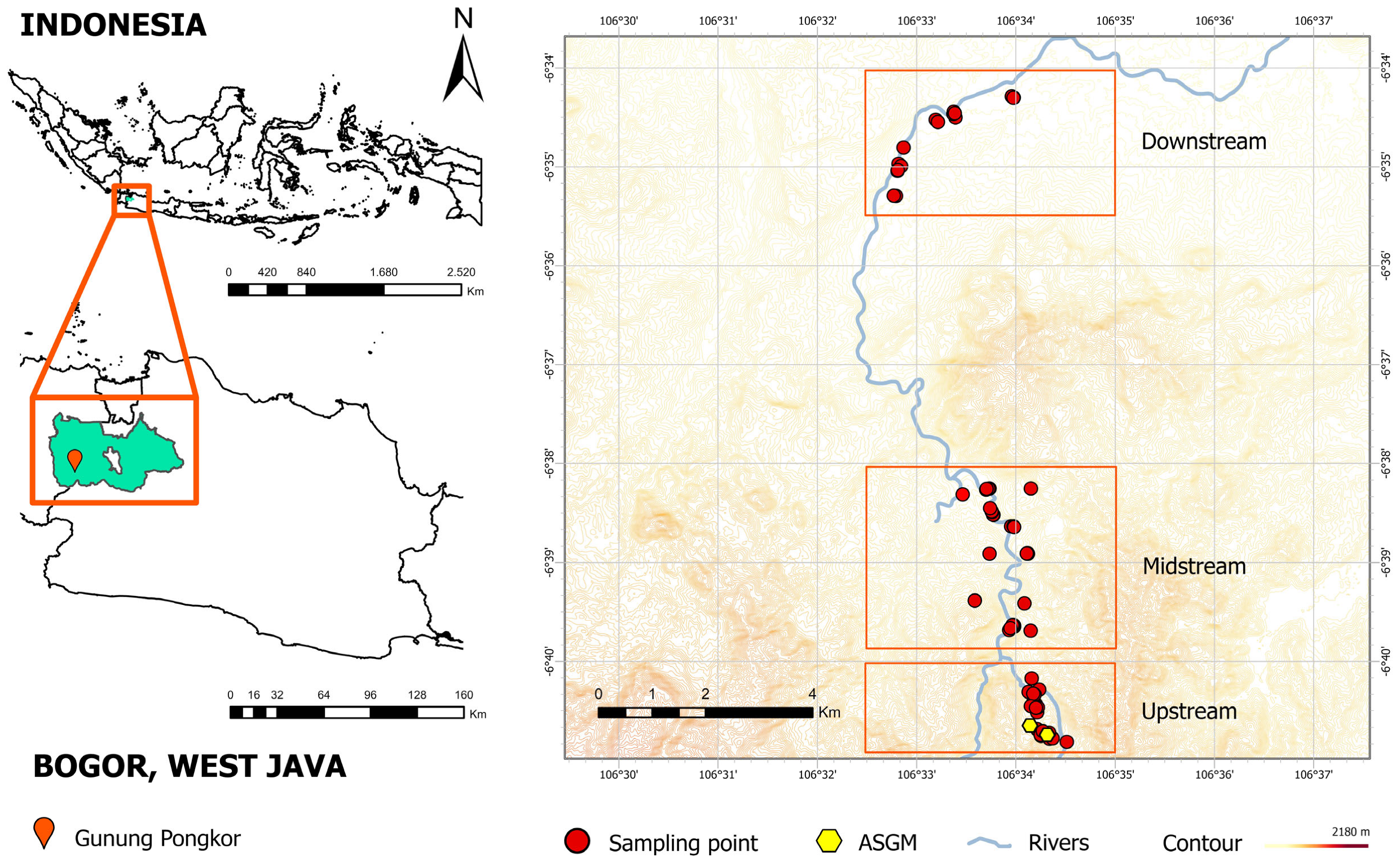
Figure 2A illustrates the geographical distribution of Hg concentration in river water surrounding the Gunung Pongkor area. Elevated levels of Hg were detected not only in the upstream area but also in both the midstream and downstream areas. Spearman’s rank analysis of Hg concentration in river water showed no significant correlation with distance from ASGM sites 1 (r = −0.065,
p = 0.792) and 2 (r = −0.070,
p = 0.775) (
Table S5). The analysis also revealed no significant correlation between Hg levels in river water and sediment (r = 0.082,
p = 0.0789) and a relationship between Hg in river water and soil (r = 0.322,
p = 0.308). This result suggests that Hg contamination is not limited to areas immediately adjacent to the ASGM sites, but rather, ASGM activities and their impacts are distributed along the entire Cikaniki River, affecting all segments of the river system.
While previous studies, such as Hiola et al. [
39], have reported that Hg concentrations in the Hulawa River are typically higher near ASGM locations and similar patterns have been observed in the Tano River Basin in Ghana [
40], the situation in the Cikaniki River appears to be different. Here, widespread and possibly informal ASGM activities, combined with hydrological processes such as sediment transport and erosion, likely contribute to a more uniform distribution of Hg along the river. Rainwater and soil erosion can wash Hg-laden sediments from multiple points along the riverbank into the water, and these sediments are then transported downstream [
41]. As a result, Hg pollution is not confined to areas near the main ASGM sites but is dispersed throughout the river system. Therefore, while proximity to mining sites often plays a significant role in Hg distribution, the diffuse nature of ASGM activities and river dynamics in the Cikaniki River lead to a more widespread impact.
In contrast, pond water and groundwater exhibit significantly lower median Hg concentrations, ranging from 0.08 to 0.14 µg/L and 0.09 to 0.16 µg/L, respectively, indicating less exposure to pollution sources.
Figure 2B,C illustrates the spatial distribution of Hg levels in ponds and groundwater, respectively. In the context of these water types, the distribution patterns in each subdomain are relatively homogeneous except for the influence of ASGM, which is hydrologically interconnected. Overall, despite the impact of ASGM operations on Hg levels, variations in Hg contamination patterns suggest the influence of several environmental factors beyond proximity to mining sites.
Based on a comparison between Hg in water with the standards established by Indonesia [
42], the levels allow up to 2.0 µg/L of Hg in river water and 1.0 µg/L in drinking water. Alarmingly, 26% of river water samples exceeded the threshold limits, while pond and groundwater samples were below the threshold limits. This result highlights the greater susceptibility of river water to Hg pollution derived from ASGM activities, considering the intensive use of Hg and the direct discharge of waste into river systems.
The correlation between Hg concentration and various physicochemical parameters was assessed using Spearman’s rank correlation coefficient across different water types given in
Table 2. A significant positive correlation existed between Hg concentration and turbidity in all samples (
r = 0.665,
p < 0.01) and river water (
r = 0.778,
p < 0.01), indicating that higher turbidity levels are associated with increased Hg concentrations, especially in river water. Turbidity often contains colloidal particles that are sufficiently small to remain suspended in water. Mercury can bind to these colloids, which may not be completely eliminated during filtration, leading to a higher measured concentration of Hg [
43]. In natural waters, colloidal Hg plays a significant role in its transport, bioavailability, and environmental fate [
44].
A moderate positive correlation was also observed between Hg and pH in all samples (
r = 0.432,
p < 0.01), suggesting that higher pH levels may influence Hg solubility and mobility by promoting the formation of more mobile and bioavailable dissolved Hg complexes [
45]. At high pH, Hg will be more likely to form soluble complexes, e.g., Hg(OH)
2 and other hydroxylated species [
45]. These complexes are more stable and stay in solution rather than precipitating or adsorbing to sediments. Alkaline conditions could also lower the binding affinity of Hg to organic matter and particles and render it more mobile and potentially more bioavailable. Thus, Hg may remain in the water column for longer and become more readily transported or taken up by aquatic organisms, increasing the environmental and health risks. In aquatic environments, Hg primarily exists as inorganic Hg (Hg
2+) and methylmercury (MeHg), a highly bioavailable, neurotoxic compound that is persistent in biological systems [
46]. While this study did not directly measure MeHg, the observed pH and turbidity conditions may facilitate its formation and mobility.
To contextualize the results, our study’s Hg concentration is compared to those of other impacted and reference sites both within Indonesia and internationally (
Table 1). Within our study area, previous research on the Cikaniki River in Bogor [
13,
14,
18,
19,
20,
21,
22,
23] reported a wider range of Hg concentration, with an upper limit of 606 μg/L [
22], exceeding the levels observed in this study. This difference likely reflects the 2017 ban on Hg use in ASGM in Indonesia [
47], suggesting a potential decrease in Hg contamination in recent years. Other Indonesian rivers impacted by ASGM have also exhibited higher Hg concentrations, including the Hulawa River in North Gorontalo [
39] and, notably, the Bone River in Gorontalo [
48], which reported extreme values. In contrast, lower mean Hg levels were found in Lebak Situ-Banten [
49] and Krueng Sabee-Aceh [
50]. As expected, reference sites in Mandailing, Natal-North Sumatra, considered uncontaminated, showed very low Hg concentrations [
10]. Gunung Pongkor stands out for showing signs of environmental improvement, likely due to regulatory actions and improved ASGM practices. This makes it an important case study for evaluating the effectiveness of Hg reduction efforts in ASGM regions.
Globally, Hg concentration in water sources near ASGM sites, such as the Insingile River in Tanzania [
51] and the Anikoko River in Ghana [
52], is generally higher than that observed in this study. However, some locations, like the Tapajos River in the Brazilian Amazon [
53], have reported extremely low Hg levels, comparable to uncontaminated sites. Overall, our results indicate that Hg concentration in the Gunung Pongkor area is elevated compared to uncontaminated reference sites but lower than those observed in other heavily polluted ASGM areas in Indonesia and internationally, highlighting that pollution influences not only current ASGM practices but also the legacy of historical contamination.
3.2. Hg Concentration in Soil
Table 3 illustrates the Hg concentration in soil along a river system and residential area, revealing a clear decreasing trend from upstream (5.51 mg/kg dw) to midstream (4.45 mg/kg) and downstream (0.62 mg/kg). This strong upstream-to-downstream gradient (
Figure 2D) suggests a point source of pollution near the upstream area, potentially from intensive land use practices like ASGM activities. This pattern aligns with previous studies that documented elevated levels of Hg in samples collected near mining operations [
10,
14,
54]. The main environmental concern with Hg accumulation in soil is its potential transformation into methylmercury (CH
3Hg), a highly toxic and bioavailable form. Inorganic Hg (Hg
2+) binds to organic matter and mineral surfaces, with its mobility and speciation influenced by environmental factors such as pH, redox conditions, and temperature. Acidic soils favor the persistence of Hg
2+, while oxygen-rich conditions can enhance its solubility. Moreover, atmospheric deposition of Hg (e.g., HgO) can contribute to soil contamination through wet and dry deposition. Rainfall and flooding can further mobilize Hg, increasing its distribution in surrounding environments [
55].
Table S5 provides a Spearman’s rank correlation for various parameters associated with distance to ASGM 1, distance to ASGM 2, and Hg concentration. Analysis showed no relationship among the parameters with Hg concentration. The observed decrease in Hg levels downstream can likely be attributed to processes such as dilution, sedimentation, or changes in soil composition affecting Hg retention. All soil samples showed Hg concentration above the standard set (0.3 mg/kg) by the Indonesian Minister of Environment and Forestry Regulation [
42]. Notably, Hg concentration in the downstream areas was above this standard, possibly due to naturally high background levels. Furthermore, agricultural practices and ASGM contribute to the mobilization of Hg-enriched soils.
Contextualizing these findings within the broader Indonesian and global landscape provides crucial insights (
Table 3). Within Indonesia, Gunung Pongkor’s upstream soils showed a higher Hg concentration than forest soils in Bogor [
21] and paddy soils in North Sumatra [
10], underscoring the severe impact of ASGM. However, the contamination levels in Gunung Pongkor were significantly lower than the extreme cases reported in Bombana-Sulawesi [
56]. Globally, comparisons with other ASGM-affected areas further illuminate the extent of Hg contamination in ASGM-affected areas. Soils from Tanzania [
51], Mauritania [
57], South Africa [
58], and Ghana (mean: 2.17 mg/kg) [
17] generally showed lower Hg concentration than those observed in Gunung Pongkor’s upstream sites.
3.3. Hg Concentration in Sediment
The median concentration of Hg in river and pond sediment samples exhibited an unusual increasing trend (
Table 4) from upstream (10.0 mg/kg dw), midstream (6.00 mg/kg dw), and downstream (64.4 mg/kg dw) (
Figure 2E). This downstream increase, also observed in previous studies [
59], suggests multiple point sources of Hg pollution along the river system, particularly in the downstream reaches. The extreme variability in Hg concentrations, especially downstream, further indicates localized pollution sources, likely related to current or historical gold mining activities [
59]. Correlation analysis demonstrated no significant correlation between the Hg concentration in sediment and each parameter (
Table S5). This lack of correlation, along with the observed downstream increase in Hg, suggests that other factors may contribute to Hg accumulation. One such factor could be the abundance of organic matter, which is often higher in soil than in river sediment. Organic matter can strongly bind Hg, reducing its mobility and promoting its retention in the soil. This binding is primarily due to the formation of stable complexes between Hg and organic compounds, particularly humic substances, which inhibit Hg release and enhance its spatial stability [
60].
Because the Indonesian government lacks specific regulations for sediment quality for Hg, the Hong Kong Interim Sediment Quality Guidelines (IHSG) (0.15 mg/kg) [
61] were utilized to assess the results. All sediment samples exceeded these guidelines.
Comparing this study’s findings with other reports from Indonesia is necessary to interpret our findings, as shown in
Table 4. This study’s median Hg concentration downstream was higher than that of the previous research in Bogor-West Java [
14], Banyumas-Central Java [
62], Ciujung-Banten [
63], and Lolayan-Bolaang Mongondow. However, they were lower than those reported in Bone Bolango-Gorontalo [
48], an area known to be heavily polluted by Hg from ASGM.
Compared with studies in other countries, Hg concentration in this study was higher than those in Gauteng-South Africa [
58], Brazilian Amazon [
53], Ghana [
40], Anka-Northwest Nigeria [
3], Northwest China [
64], and Central Brazil [
65]. These findings underscore the critical need for comprehensive environmental monitoring, the stringent regulation of ASGM practices, and targeted remediation efforts in heavily impacted areas like Gunung Pongkor.
3.4. Hg Concentration in Fish
Concentration of Hg in fish from the Gunung Pongkor area is shown in
Table 5. Median Hg concentrations in fish from ponds were 0.755 mg/kg dw in the upstream area, 0.700 mg/kg dw in the midstream area, and 0.392 mg/kg dw in the downstream area.
Some variation in Hg concentrations was observed among the ponds from the upstream–downstream areas (
Figure 2F, statistical analysis revealed no significant differences (
p > 0.05), suggesting that spatial variability was limited under current conditions. Likewise, Hg concentration in pond water (
p = 0.112) and fish length (
p = 0.182) did not differ significantly between sites, suggesting that these factors were relatively uniform across sampling sites. However, a significant difference was observed in fish weight (
p = 0.03), implying that fish weight varied meaningfully among the sites, even though Hg exposure and other measured environmental parameters did not show significant spatial trends. This spatial variability aligns with findings from previous studies. For example, Lavoie et al. [
66] discussed how local geochemistry and food web structure influence Hg bioaccumulation in fish, explaining the observed variations across sampling sites. Eagles-Smith et al. [
67] highlighted the complexity of factors (fish species, fish size, and habitats) affecting Hg concentrations in freshwater fish.
Correlation analysis revealed significant positive correlations between Hg concentrations in fish muscle and both pond water (
r = 0.421,
p < 0.05) and pond sediment (
r = 0.520,
p < 0.05), indicating that both are important sources of Hg exposure for fish in the Gunung Pongkor area. Fish can absorb heavy metals, including Hg, through their gills and skin via ion exchange, consuming contaminated food, or through adsorption into their tissues [
68]. No significant correlation was found between the Hg concentration in fish tissue and either fish length (
r = 0.202) or fish weight (
r = 0.262).
At a wet weight basis, the median concentrations of Hg in tilapia from upstream (0.156 mg/kg ww), midstream (0.140 mg/kg ww), and downstream (0.082 mg/kg ww) were all below the threshold level of 0.5 mg/kg ww according to the Indonesian Food and Drug Administration Regulation No. 09 [
69]. This result indicates that the fish product has a permitted level of Hg pollutant.
A comparison of Hg concentration in fish from Gunung Pongkor with other studies in Indonesia and internationally is shown in
Table 5. Within Indonesia, this study exhibited a higher median Hg level compared to similar species in Gorontalo [
70] and Lolayan-Bolaang Mongondow [
71], indicating a higher degree of Hg contamination. However, these levels were substantially lower than those found in West Sumbawa’s Tilapia fish [
72]. The stark contrast with the minimal contamination (0.0942 mg/kg ww) observed in the reference site at Tatelu-North Sulawesi [
73] underscores the impact of human activities, likely ASGM, on the Hg level in Gunung Pongkor. Internationally, the level of Hg found in fish from Gunung Pongkor was relatively low when compared to the high levels of Hg measured in Ghana from the study of 13 fish species, including tilapia from rivers surrounding gold mining operations [
74]. Additionally, Hg levels in tilapia from fish ponds in Migori County in Kenya were higher than those from Gunung Pongkor [
75]. Conversely, Hg levels in Gunung Pongkor exceed those observed in
Piaractus brachypomus from Madre de Dios, Peru [
76]. Notably, the range of Hg concentration in Gunung Pongkor falls within the broader spectrum documented in Puerto Narino, Southern Colombia, for 24 species of fish from the Amazon River [
77], highlighting the global variability in fish Hg contamination. These comparisons emphasize the influence of local factors such as geology, anthropogenic activities, and environmental conditions on Hg bioaccumulation in fish. The findings underscore the critical need for continued monitoring and region-specific assessments to inform public health guidelines and develop targeted environmental management strategies to mitigate Hg pollution in aquatic ecosystems.
Table 1.
Comparison of Hg concentration (µg/L) in water with other studies around ASGM areas.
Table 1.
Comparison of Hg concentration (µg/L) in water with other studies around ASGM areas.
| Location | Remarks | n | Mean | Range | Median | Reference |
|---|
| Indonesia | | | | | | |
| Gunung Pongkor—Bogor, West Java | | | | | | This study |
| Upstream | River water (Ciguha—Cikaniki River) | 7 | 0.95 | 0.10–2.48 | 0.28 | |
| Midstream | | 7 | 1.63 | 0.06–4.49 | 0.28 | |
| Downstream | | 5 | 1.64 | 0.08–4.35 | 1.65 | |
| Upstream | | 3 | 0.16 | 0.11–0.23 | 0.14 | |
| Midstream | Pond water | 7 | 0.09 | 0.06–0.14 | 0.08 | |
| Downstream | Groundwater | 3 | 0.10 | 0.08–0.12 | 0.10 | |
| Upstream | 3 | 0.16 | 0.09–0.23 | 0.16 |
| Midstream | 3 | 0.08 | 0.07–0.10 | 0.09 |
| Downstream | 6 | 0.11 | 0.09–0.17 | 0.10 |
| West Java | 2001—Cikaniki River | 3 | 3.75 * | 2.74–4.86 | 3.63 * | [13] |
| 2002—Cikaniki River | 3 | 0.74 * | 0.37–1.13 | 0.72 * |
| Bogor—West Java Upstream | Cikaniki River | 1 | 0.44 | - | - | [19] |
| Midstream | | 1 | 0.30 | - | - | |
| Bogor—West Java Upstream | Cikaniki River | 1 | 0.50 | - | - | [18] |
| Bogor—West Java | Cikaniki River | 2 | - | 0.119–0.218 | - | [20] |
| Bogor—West Java | Cikaniki River | 5 | 3.46 * | 0.09–9.07 | 0.36 * | [14] |
| Bogor—West Java | Cikaniki River | 3 | - | 1.35–1.57 | - | [23] |
| Bogor—West Java | Cikaniki River | 9 | 3.49 * | 0.40–9.60 | 0.66 * | [21] |
| Bogor—West Java | Cikaniki River | | | | | [22] |
| March 2013 | 13 | 4.60 * | 0.002–17.4 | 0.95 * |
| March 2014 | 9 | 10.3 * | 1.20–24.0 | 8.80 * |
| September 2014 | 11 | 4.31 * | 0.003–12.0 | 2.32 * |
| December 2014 | 12 | 4.40 * | 0.12–15.5 | 4.44 * |
| August 2015 | 11 | 87.7 * | 0.36–606 | 9.88 * |
| December 2015 | 9 | 1.81 * | 0.24–9.87 | 0.63 * |
| November 2016 | 7 | 1.17 * | 0.43–1.94 | 1.07 * |
| November 2017 | 8 | 2.76 * | 0.41–7.43 | 1.40 * |
| North Gorontalu—Gorontalo | Hulawa River | 5 | 8.26 | 0.10–21.3 | 1.30 * | [39] |
| Bone Bolango—Gorontalo | Bone River | 11 | 345 | 16.0–2080 | 71.0 | [48] |
| Banyumas—Central Java | Tajum River | 7 | 1003 | 100–1900 | - | [62] |
| Lebak situ—Banten | Rice Field Water | 12 | 0.142 | 0.009–0.927 | - | [49] |
| Aceh Jaya—Aceh | Krueng Sabee, Panga, and Teunom River | 18 | 0.097 | 0.007–0.333 | 0.056 | [50] |
| Jayapura—Papua | Jabawi, Kleblow, and Komba River | 4 | 41.3 | 22.0–55.0 | 44.0 | [78] |
| Nauli and Simalagi villages—Mandailing Natal, North Sumatra | Groundwater | 16 | 0.62 | 0.45–1.3 | - | [10] |
| Drinking water | 16 | 0.59 | 0.45–0.75 | - |
| Reference sites—Mandailing Natal, North Sumatra | Drinking water—uncontaminated area | 3 | 0.04 | - | - | [10] |
| Groundwater—uncontaminated area | 3 | 0.06 | - | - |
| Other Countries | | | | | | |
| Northwest China | Xiyu River | 17 | 1.34 | 0.07–7.59 | - | [64] |
| Bono, Bono East, Ahafo—Ghana | River Tano Basin | 9 | 0.045 | BDL–0.19 | 0.014 | [40] |
| Pestea Huni Valley—Ghana | Anikoko, Abodwesh, Ankobra, Amenkime, Dinyame, Anfoe, Woawora, Benyan, and Mansi River | 70 | - | 132–866 | - | [52] |
| Randfontein, Gauteng—South Africa | Tailing dams | 7 | - | 0.032–0.067 | - | [58] |
| Streams | - | - | 0.004–0.068 | - |
| Wetlands | - | - | 0.007–0.012 | - |
| Abu Hamad—Sudan | Nile River | 7 | - | 0.27–3.26 | - | [79] |
| River Nile State, Darmali—Sudan | Groundwater and tap water are drawn from the Nile River | 8 | 0.26 | - | - | [80] |
| Rwamagasa, Geita—Tanzania | Insingile River as a water source | 24 | 47.8 | <1.0–920 | 20 | [51] |
| Brazilian Amazon | Unfiltered water of Tapajos River | 47 | 0.005 | 0.007–0.024 | - | [53] |
| Central Brazil | Araguaia River Floodplain | 98 | 0.002 | 0.0001–0.004 | - | [65] |
Table 2.
Spearman rank correlation coefficient for Hg with the physicochemical parameters of the water.
Table 2.
Spearman rank correlation coefficient for Hg with the physicochemical parameters of the water.
| | pH | Temperature | DO | TDS | Turbidity | Salinity | EC |
|---|
| River water | 0.061 | −0.411 | 0.293 | −0.097 | 0.778 ** | 0.074 | −0.027 |
| Pondwater | 0.135 | 0.029 | −0.186 | 0.424 | na | 0.258 | 0.450 |
| Groundwater | 0.534 | 0.432 | −0.243 | 0.036 | na | 0.188 | 0.358 |
| All sample | 0.432 ** | −0.192 | 0.086 | −0.032 | 0.665 ** | 0.016 | 0.167 |
Table 3.
Comparison of Hg concentration (mg/kg dw) in soil with other studies around ASGM areas.
Table 3.
Comparison of Hg concentration (mg/kg dw) in soil with other studies around ASGM areas.
| Location | Remarks | n | Mean | Range | Median | Reference |
|---|
| Indonesia | | | | | | |
| Gunung Pongkor—Bogor, West Java | | | | | | This study |
| Upstream | Residential areas and riverbank soil | 13 | 18.0 | 0.439–144 | 5.51 | |
| Midstream | 5 | 3.60 | 1.18–6.04 | 4.45 | |
| Downstream | 4 | 1.10 | 0.420–2.78 | 0.62 | |
| Bogor—West Java | Forest soil | 34 | 1.89 * | 0.11–9.35 | - | [14] |
| Paddy field | 15 | 15.3 * | 1.03–73.0 | - |
| Bogor—West Java | Forest soil | 7 | 0.69 * | 0.11–2.22 | - | [21] |
| Paddy field soil | 9 | 9.00 | 0.40–24.9 |
| Lebak Situ—Banten | Rice field soil | 15 | 0.124 | 0.212–2.47 | - | [49] |
| Bombana—Sulawesi | ASGM area | 8 | 390 | 12.0–2500 | 63.0 | [56] |
| Mining commercial area | 12 | 13.0 | 0.00–45.0 | 2.40 |
| Nagan Raya—Aceh | Soil riverbank | 3 | 0.278 | 0.271–0.328 | - | [81] |
| Nauli and Simalagi village, Mandailing Natal—North Sumatra | Paddy soil | 20 | 5.60 | 0.26–5.80 | - | [10] |
| Farm soil | 20 | 19.0 | 0.18–100 | - |
| Reference site—Banjarbaru, South Kalimantan | Agriculture soil—uncontaminated area | 6 | 0.02 | 0.01–0.04 | - | [32] |
| Other Countries | | | | | | |
| Obuasi, Ashanti—Ghana | Farmland soil | 9 | 2.17 | 2.10–2.25 | - | [82] |
| | Soil tailing | - | 0.855 | 0.853–0.858 | | |
| Obuasi—Ghana | Soil around Tweapease | 3 | 3.68 | 3.54–3.88 | - | [17] |
| Soil around Nyamebekyere | 3 | 2.03 | 2.01–2.05 | - |
| Soil around Ahansonyewodea | 3 | 1.33 | 1.29–1.39 | - |
| Migori, Transmara—Kenya | Soil riverbank | 94 | 0.14 | 0.02–1.10 | 0.10 | [83] |
| Nouakchott, Chami Town—Mauritania | Natural soils, soil from residential areas, and soil from the ASGM area | 180 | - | 0.002–9.3 | - | [57] |
| Anka—Northwest Nigeria | Soil | 42 | 0.85 | - | - | [3] |
| Randfontein, Gauteng—South Africa | Tailing dams | 11 | - | 0.89–6.76 | - | [58] |
| Community soil | - | - | 0.43–0.97 | - |
| Garden soil | - | - | 0.47–1.02 | - |
| Darmali—Sudan | Agricultural soil | 18 | - | - | 0.057 | [80] |
| Residential area | 10 | - | - | 0.044 |
| Tailing | 6 | - | - | 9.60 |
| Mbogwe, Geita—Tanzania | Agricultural soil | 12 | 0.017 | 0.008–0.026 | - | [84] |
| Rwamagasa, Geita—Tanzania | Soil | 92 | 0.058 | 0.01–1.76 | - | [51] |
Table 4.
Comparison of Hg concentration (mg/kg dw) in sediment with other studies around ASGM areas.
Table 4.
Comparison of Hg concentration (mg/kg dw) in sediment with other studies around ASGM areas.
| Location | Remarks | n | Mean | Range | Median | Reference |
|---|
| Indonesia | | | | | | |
| Gunung Pongkor—Bogor, West Java | | | | | | This study |
| Upstream | Ciguha River to Cikaniki River | 7 | 12.9 | 0.920–31.7 | 10.0 | |
| Midstream | 9 | 16.1 | 1.17–67.3 | 6.00 | |
| Downstream | 4 | 70.3 | 2.60–150 | 64.4 | |
| Bogor—West Java | Cikaniki River | 1 | 0.10 | - | - | [18] |
| West Jawa | Cikaniki River | 2 | - | 0.83–1.07 | - | [20] |
| Bogor—West Java | Cikaniki River | 8 | 19.7 * | 0.093–85.2 | - | [14] |
| Bogor—West Java | Cikaniki River | | | | | [22] |
| March 2013 | 9 | 51.0 * | 29.0–79.2 | 43.4 * |
| September 2014 | 9 | 5.56 * | 0.20–15.8 | 4.67 * |
| December 2014 | 12 | 21.4 * | 8.50–40.7 | 20.0 * |
| December 2015 | 8 | 34.0 * | 9.50–71.8 | 22.0 * |
| November 2016 | 7 | 36.1 * | 9.70–93.4 | 23.3 * |
| November 2017 | 9 | 23.8 * | 7.00–49.9 | 22.9 * |
| Bone Bolango—Gorontalo | Bone River | 11 | 186 | BDL–790 | - | [48] |
| Banyumas—Central Java | Tajum River | 7 | 9.75 | 6.90–11.8 | - | [62] |
| Ciujung—Banten | Ciujung Watershed | 11 | 0.61 | 0.02–0.91 | 0.62 | [63] |
| Lolayan—Bolaang Mongondow | Bakan River | 3 | 3.26 | - | - | [71] |
| Reference site—Buru, Maluku | Upstream of Waelata River—uncontaminated area | 3 | 0.023 | 0.021–0.025 | - | [33] |
| Other Countries | | | | | | |
| Northwest China | Xiyu River | 17 | 2.69 | 0.27–9.16 | - | [64] |
| Bono, Bono East, Ahafo—Ghana | River Tano Basin | 9 | 1.24 | BDL–4.80 | 1.00 | [40] |
| Anka—Northwest Nigeria | Stream sediment | 22 | 2.12 | - | - | [3] |
| Randfontein, Gauteng—South Africa | Tailing dams | 7 | - | 0.65–1.99 | - | [58] |
| Streams | - | - | 0.60–1.36 | - |
| Wetlands | - | - | 0.68–1.36 | - |
| Brazilian Amazon | Superficial sediment of Tapajos River | 27 | 0.074 | 0.019–0.155 | - | [53] |
| Central Brazil | Araguaia River Floodplain | 98 | 0.044 | 0.010–0.107 | - | [65] |
Table 5.
Comparison of Hg concentration (mg/kg dw) in fish with other studies around ASGM areas.
Table 5.
Comparison of Hg concentration (mg/kg dw) in fish with other studies around ASGM areas.
| Location | Remarks | n | Mean | Range | Median | Reference |
|---|
| Indonesia | | | | | | |
| Gunung Pongkor—Bogor, West Java | | | | | | This study |
| Upstream | Tilapia (Orechromis niloticus) from fish ponds | 4 | 0.693 | 0.260–1.000 | 0.755 | |
| Midstream | 3 | 0.670 | 0.259–1.05 | 0.700 | |
| Downstream | 5 | 0.522 | 0.268–1.23 | 0.392 | |
| Gorontalo | Tilapia (Oreochromis niloticus) from Limboto Lake | 6 | 0.283 * | 0.0471 *–0.424 * | 0.283 * | [70] |
| Lolayan—Bolaang Mongondow | Tilapia (Oreochromis niloticus) from Bakan river | 3 | 0.382 * | - | - | [71] |
| West Sumbawa | Tilapia (Oreochromis niloticus) from Rawa Taliwang Lake | 4 | 3.44 * | 3.06 *–3.82 * | - | [72] |
| Reference—Tatelu, North Sulawesi | Freshwater fish from Toldano River–uncontaminated area | 6 | 0.0942 * | - | - | [73] |
| Other Countries | | | | | | |
| Ghana | 13 species of fish from rivers in gold mining areas | 17 | 1.18 * | - | - | [74] |
| Migori County—Kenya | Oreochromis niloticus from fish ponds | 10 | 2.07 * | 0.848 *–4.33 * | 1.79 * | [75] |
| Madre de Dios—Peru | Piaractus brachypomus from farmed fish | 111 | 0.236 * | 0.0471 *–1.083 * | - | [76] |
| Puerto Narino—Southern Colombia | 24 species of fish from the Amazon River | 102 | 0.942 * | 0.0471 *–6.59 * | - | [77] |
3.5. Hg Concentration in Cassava
The Hg concentration in cassava roots and leaves from various sampling locations are depicted in
Table 6 and
Table 7, respectively. The median Hg concentrations in cassava roots were 0.488 mg/kg dw upstream, 1.05 mg/kg dw midstream, and 0.108 mg/kg dw downstream. Cassava leaves show median Hg concentrations of 5.40 mg/kg dw upstream, 1.98 mg/kg dw midstream, and 0.860 mg/kg dw downstream.
The geographical distribution of Hg in cassava roots and leaves (
Figure 2G,H) showed a high concentration for both in the upstream area (5.09 mg/kg dw in roots and 8.84 mg/kg dw in leaves), likely due to the proximity of ASGM workplaces. A statistical test revealed significant differences in Hg among areas for cassava roots (
p = 0.017); in contrast, no significant differences were found for cassava leaves. Variability was observed within each area, particularly in upstream samples, which may be attributed to aerial Hg sources, consistent with observations by Adjorlolo-Gasokpoh et al. [
85]. Of particular interest is the marked variability observed across upstream samples, especially among certain root samples, which displayed low concentrations. This observation underscores the complex dynamics of Hg uptake and distribution in cassava plants. The generally lower Hg concentration in downstream samples suggests a dilution effect or reduced Hg bioavailability further from the potential source [
85].
On a wet weight basis, the concentration of Hg in cassava roots from upstream (0.193 mg/kg ww), midstream (0.415 mg/kg ww), and downstream (0.043 mg/kg ww) samples exceeded the threshold level of 0.03 mg/kg ww according to Indonesian Food and Drug Administration Regulation No. 9 [
69]. All cassava leaves from upstream (1.38 mg/kg ww), midstream (0.522 mg/kg ww), and downstream (0.263 mg/kg ww) exceeded the threshold.
Mercury concentration in cassava leaf (
n = 10) was significantly higher than in cassava root (
n = 10) (
p < 0.001) (
Figure 3A). This pattern, consistent with findings from other gold mining-affected regions [
51,
85], can be attributed to both atmospheric Hg
0 uptake through stomata [
86] and soil-to-plant transfer [
87]. Soil characteristics, such as organic matter (OM), pH, and microbial activity, can influence Hg speciation and bioavailability to plants [
88]. Although the atmospheric Hg concentration plays a key role in leaf accumulation, particularly under elevated ambient concentration, soil Hg content also contributes to total Hg uptake [
87]. Approximately 10% of the Hg concentration in the soil can be transported to the leaves, especially when atmospheric Hg levels are low [
87]. This study found no significant correlation between the soil and leaf Hg concentrations. This indicates that atmospheric deposition may be the primary source of Hg in cassava leaves.
The comparison of the median Hg concentration in cassava roots in Gunung Pongkor with other regions in Indonesia and internationally reveals significant variations in contamination levels associated with ASGM activities (
Table 6). Within Indonesia, Gunung Pongkor’s median Hg level was lower than those in Sukabumi-West Java [
89] but higher than those in Palu-Central Sulawesi [
90]. In the international context, Gunung Pongkor’s contamination level was generally higher than those reported in Ghana [
17,
87], Tanzania [
51], and Uganda [
91]. Conversely, Hg concentration found in the downstream area of this study was lower than that recorded in El Bagre, Colombia [
92]. Notably, Hg levels in both the upstream and downstream areas of Gunung Pongkor were higher than those observed in El Bagre. These comparisons highlight how ASGM activities affect Hg contamination in cassava roots differently across regions. Local assessments and targeted strategies are essential to address Hg pollution. The data from Gunung Pongkor shows the serious environmental challenges of ASGM in Indonesia, stressing the importance of effective pollution control measures.
Meanwhile, a comparison of the median Hg concentration in cassava leaves in Gunung Pongkor with other places in Indonesia and around the world is revealed in
Table 7. Mercury concentration upstream was lower than that found in Bombana, Sulawesi, around the ASGM area [
56], yet higher than those near commercial mining areas, as well as in Sukabumi and Mandailing Natal [
10,
89]. In contrast, the midstream and downstream levels at Gunung Pongkor were lower than those observed in Mandailing Natal, North Sumatra [
10]. On a global scale, the Hg concentration at Gunung Pongkor, particularly in upstream areas, was markedly elevated compared to Bogoso, Ghana [
85], Mbogwe, and Rwamagasa in Geita, Tanzania [
51,
84], as well as Eastern Uganda [
91]. These findings underscore the significant effects of ASGM activities on Hg accumulation in the environment, especially in areas where ASGM is located in Sukabumi.
Table 6.
Comparison of Hg concentration (mg/kg dw) in cassava roots with other studies around ASGM areas.
Table 6.
Comparison of Hg concentration (mg/kg dw) in cassava roots with other studies around ASGM areas.
| Location | Remarks | n | Mean | Range | Median | Reference |
|---|
| Indonesia | | | | | | |
| Gunung Pongkor—Bogor, West Java | | | | | | This study |
| Upstream | Residential area and riverbank | 6 | 1.75 | 0.139–5.09 | 0.488 | |
| Midstream | 4 | 1.18 | 0.343–2.28 | 1.05 | |
| Downstream | 4 | 0.106 | 0.0973–0.110 | 0.108 | |
| Sukabumi—West Java | Ball mill area | 2 | 31.1 | - | - | [89] |
| Palu—Central Sulawesi | Agricultural area | 4 | 0.33 | - | - | [90] |
| Other Countries | | | | | | |
| Bogoso—Ghana | River Bogo riverbank | 1 | 0.079 | - | - | [85] |
| Obuasi—Ghana | Tweapease, farmland | 3 | 0.331 | 0.321–0.345 | - | [17] |
| Nyamebekyere, farmland | 3 | 0.243 | 0.236–0.248 |
| Ahansonyewodea, farmland | 3 | 0.115 | 0.100–0.130 |
| Rwamagasa, Geita—Tanzania | Residential area | 14 | 0.003 | 0.001–0.008 | - | [51] |
| Bugiri, Busia, and Namayingo—Uganda | Farmland area | 3 | 0.02 | 0.004–0.042 | - | [91] |
| El Bagre, Bajo Cauca—Colombia | Chards or cropped areas close to local inhabitants’ homes | 12 | 0.39 | - | - | [92] |
Table 7.
Comparison of Hg concentration (mg/kg dw) in cassava leaves with other studies around ASGM areas.
Table 7.
Comparison of Hg concentration (mg/kg dw) in cassava leaves with other studies around ASGM areas.
| Location | Remarks | n | Mean | Range | Median | Reference |
|---|
| Indonesia | | | | | | |
| Gunung Pongkor—Bogor, West Java | | | | | | This study |
| Upstream | Residential area and riverbank | 6 | 4.84 | 0.750–8.84 | 5.40 | |
| Midstream | 4 | 2.16 | 0.650–4.02 | 1.98 | |
| Downstream | 4 | 0.945 | 0.350–1.71 | 0.860 | |
| Bombana—Sulawesi | ASGM | 8 | 9.90 | 1.50–2500 | 5.90 | [56] |
| Mining commercial area | 6 | 3.20 | 0.00–45.0 | 2.20 |
| Sukabumi—West Java | Ball mill area | 7 | 4.61 | - | - | [89] |
| Mandailing Natal—North Sumatra | Agricultural area | 6 | 2.00 | - | - | [10] |
| Other Countries | | | | | | |
| Bogoso—Ghana | River Bogo riverbank | 1 | 0.136 | - | - | [85] |
| Mbogwe, Geita—Tanzania | Farmland area | 4 | 0.15 | 0.08–0.34 | - | [84] |
| Rwamagasa, Geita—Tanzania | Residential area | 14 | 0.061 | 0.008–0.167 | - | [51] |
| Bugiri, Busia, and Namayingo—Eastern Uganda | Farmland area | 3 | 0.11 | 0.05–0.15 | - | [91] |
3.6. Geo-Accumulation Index (Igeo) in Soil and Sediment
The Igeo index (
Figure 4) was used to assess Hg contamination in soil across sampling points from upstream to downstream, with values ranging from 1.15 (class 2) to 3.68 (class 4), indicating varying degrees of contamination. Upstream sites exhibited Igeo values between 1.17 and 3.68, categorized as moderately to heavily contaminated. Specifically, 31% of upstream sampling points were classified as moderately contaminated (class 2), 62% as moderately to heavily contaminated (class 3), and 8% as heavily contaminated (class 4). Notably, sampling point S7 (upstream) recorded the highest Igeo value (3.68), suggesting severe contamination likely due to nearby ASGM activities. In the midstream area, Igeo values ranged from 1.59 to 2.30, with 40% of sites moderately contaminated and 60% moderately to heavily contaminated. Downstream Igeo values ranged from 1.15 to 1.97, and all sampling points fell into class 2, indicating moderate contamination. This spatial pattern reveals a pollution gradient, with higher contamination in the upstream sample closely associated with ASGM activity, and decreasing levels downstream, likely due to dilution and/or dispersion processes. The I
geo value also appears to be influenced by land use, where areas dominated by ASGM activities, particularly upstream (
Figure S3A), showed higher contamination indices compared to midstream and downstream zones that included more agricultural and residential land uses.
Similar to soil, I
geo values in sediment (
Figure 4) indicated varying Hg enrichment levels across sampling locations, ranging from 1.43 to 3.64. Upstream sediment had I
geo values ranging from 1.43 to 3.24, with 43% classified as moderately contaminated (class 2) and 57% as moderately to heavily contaminated (class 3). Midstream I
geo values ranged from 1.53 to 3.29, with sites classified as 33% moderately contaminated (class 2), 44% moderately to heavily contaminated (class 3), and 22% heavily contaminated (class 4). Downstream I
geo values ranged from 1.88 to 3.64, with 50% classified as moderately contaminated (class 2) and 50% as heavily contaminated (class 4). This distribution suggests that sediment contamination is influenced by both intrinsic factors and anthropogenic activities. Some midstream and downstream areas showed higher contamination than that expected from upstream sources alone, potentially due to localized pollution events or pollutant transport and sedimentation patterns.
3.9. Health Risk Assessment
To assess the health risks associated with Hg exposure from various environmental samples (water, soil, sediment, fish, and cassava plants), we applied the USEPA model to calculate the HQ (
Figure 5) and HI (
Figure 6), considering multiple exposure pathways including ingestion, dermal, and inhalation for both children and adults. An HQ or HI value exceeding one indicates the potential health risks, while a value below one suggests acceptable exposure levels. The analysis of 44 water samples showed generally low risk, with HQ values below one. However, some locations, particularly those near ASGM activities, showed elevated HQ for children. This discrepancy highlights that HQ values are influenced by exposure assumptions (e.g., ingestion rate, duration, body weight) and that low HQ can occur even when Hg concentrations exceed regulatory limits. Importantly, water quality standards are designed to be highly protective, so exceedances signal the need for monitoring rather than an immediate health threat.
In terms of soil exposure, children were notably at risk, primarily through ingestion, accounting for 10% of cases. In contrast, adults showed no significant risk, as all HQ values remained below one. The HI presented varying risk levels across the sampled sites, with particular areas, especially those adjacent to ASGM activities (upstream area), displaying high-risk levels for children. Whereas, downstream regions indicated minimal risk. Sediment exposure analysis pointed to significant health risks, predominantly through ingestion. Several sites recorded high HQ and HI values for children, with adults also exhibiting marginally elevated values, necessitating further attention. By examining fish from 12 locations, it was observed that children faced significantly greater risks compared to adults, with 79% of sites exceeding safe HQ levels for children, in contrast to 45% for adults. Certain fish samples demonstrated extraordinarily high HQ values for children, underscoring their heightened vulnerability. The evaluation of cassava roots predominantly indicated low risk, with HQ values remaining below one. Nonetheless, specific areas reported HQ values surpassing safety thresholds for children and slightly exceeding them for adults. Conversely, a considerable portion of cassava leaves exhibited HQ values that exceeded safe limits, thereby posing risks for both demographics, accounting for 57% of samples that exceeded acceptable thresholds for children.


 ,
, 