Interpretation of a Machine Learning Model for Short-Term High Streamflow Prediction

Abstract

Machine learning models are increasingly used for streamflow prediction due to their promising performance. However, their data-driven nature makes interpretation challenging. This study explores the interpretability of a Random Forest model trained on high streamflow events from a hydrological perspective, comparing methods for assessing feature influence. The results show that the mean decrease accuracy, mean decrease impurity, Shapley additive explanations, and Tornado methods identify similar key features, though Tornado presents the most notable discrepancies. Despite the model being trained with events of considerable temporal variability, the last observed streamflow is the most relevant feature accounting for over 20% of importance. Moreover, the results suggest that the model identifies a catchment region with a runoff that significantly affects the outlet flow. Accumulated local effects and partial dependence plots may represent first infiltration losses and soil saturation before precipitation sharply impacts streamflow. However, only accumulated local effects depict the influence of the scarce highest accumulated precipitation on the streamflow. Shapley additive explanations are simpler to apply than the local interpretable model-agnostic explanations, which require a tuning process, though both offer similar insights. They show that short-period accumulated precipitation is crucial during the steep rising limb of the hydrograph, reaching 72% of importance on average among the top features. As the peak approaches, previous streamflow values become the most influential feature, continuing into the falling limb. When the hydrograph goes down, the model confers a moderate influence on the accumulated precipitation of several hours back of distant regions, suggesting that the runoff from these areas is arriving. Machine learning models may interpret the catchment system reasonably and provide useful insights about hydrological characteristics.

1. Introduction

Machine learning (ML) predictive models have become popular in the recent decade for hydrological prediction [1,2,3]. One of the fields where the ML models have received considerable attention due to their promising results is streamflow prediction, where they have been shown to reach a higher accuracy than conventional physically based models [4,5,6,7]. The ML models extract valuable information from the data by finding relationships between features (inputs, variables of the model, generally including rainfall and streamflow observations) and outputs (targets or predictions, typically streamflow) by employing a training procedure [8,9,10]. The combination of a set of values of the features that correspond to a specific output is called an instance. However, the ML models are difficult to interpret due to their nature of being purely based on data [11,12]. Their complexity, flexibility, and the possibility of accounting for input interaction result in improved performance but prevent conventional analysis methods from being applicable. In linear regression, the strength of each feature is proportional to its corresponding regression coefficient, leading to straightforward interpretation [13], or even by a Pearson correlation coefficient, as Khosravi et al. [14] applied to estimate the most influential features in a streamflow model. Such approaches do not apply to ML models. To overcome this issue, a number of methods have been proposed for interpreting ML models. They can be classified into three groups [15]: first, general analysis (also called feature importance), which attempts to show insights about how the model works globally and how important the different features are for the output; second, partial dependence analysis, which shows the effect of the different values that a feature can adopt in the whole model; third, local analysis, which is focused on how the model relies on a feature to produce a single output. These feature interpretation techniques have been applied to streamflow models.

Pham et al. [16] evaluated the general effect of features in an ML model for daily streamflow prediction by employing measures of importance such as mean decrease accuracy (MDA) and mean decrease impurity (MDI) from the Random Forest (RF) algorithm. The research showed that the most relevant feature was the streamflow of previous time steps, which is related to the similarities between streamflow values in time. On the other hand, the precipitation exhibited a reduced effect on the output, which might be related to the abundant values of zeros. Shortridge et al. [17] employed a partial dependence analysis and also reported moderate relevance of precipitation in ML models for daily streamflow as well as a monotonic relation between this feature and the output. Lin et al. [10] used the Shapley Additive Explanations (SHAP) [18] to estimate that the most relevant feature in general was the streamflow one hour from the prediction time. They also found a negative contribution of some variables in the model, which were associated with a reduction in the output. Similar results employing SHAP were obtained by Liu et al. [19] for an extreme gradient boosting model for a one-month ahead streamflow prediction model. They saw that the streamflow of some steps back from the prediction time and local meteorological features were the most relevant for their model. Streamflow one day from the prediction time and accumulated precipitation were the most relevant features employing Long Short-Term Memory and RF models in the studies developed by Sushanth et al. [20] and Vilaseca et al. [21], respectively, based on SHAP results. Even SHAP has been used in hybrid models (a combination of physically based and ML models) to estimate the variables with the highest influence [22]. SHAP has been applied mainly to see the average impact of the features in the models in the previous studies. However, an important utility of this methodology is that it can measure the contribution of the features locally in a single prediction. Therefore, it is possible to analyze the effect of the features at different points of the hydrograph (for example), but this has been barely explored in the streamflow prediction models. Other authors have employed feature importance techniques as a mechanism for feature selection. Abbasi et al. [23] and S. Liu et al. [24] employed the MDA of RF models to compute the importance of a broad group of features and selected a reduced number of them for their streamflow prediction models.

From previous studies, little hydrological knowledge about the catchment system was extracted based on the interpretation of the feature influence on the ML models. Few works have studied this topic. Mushtaq et al. [12] used SHAP to study glacier-fed catchments. They could see that the model correctly interpreted zero degrees Celsius as the threshold of the temperature that is positively related to the increments of streamflow onwards. Núñez et al. [25] found that features (meteorological and streamflow) of the neighboring catchments were related to the streamflow prediction one month ahead in their study catchment by applying several techniques (e.g., MDA, partial dependence, and SHAP), although it remains complex to give a hydrological interpretation of that result due to the lack of information in their case. Among the previous studies, only one used several interpretation techniques. It is still a little-addressed topic in the streamflow prediction area, which is a more explored topic in other areas such as structural analysis [26,27,28]. Moreover, the gap is stressed considering the study of high streamflow events, which are relevant for flood mitigation purposes as well as the feature contribution on a short-term ML model (hours ahead), which is still little explored. Consequently, the current research applies a short-term high streamflow prediction model with two main objectives: first, interpreting from an engineering and hydrological perspective, the feature effect on an RF model in terms of general, partial dependence, and local analysis; second, discussing the similarities and differences among the results of several interpretation methods, paying attention to their mathematical description.

2. Materials and Methods

2.1. Methodology

Streamflow and precipitation data from high streamflow events are collected to train an RF model for short-term (three hours ahead) streamflow prediction in the study area. Once the model is trained, three model interpretation aspects are covered: general, partial dependence, and local. The general influence of the features in the model is evaluated using the MDI, MDA (both broadly implemented in the original version of the RF algorithm [29,30,31]), and Tornado methods [32]. The partial dependence analysis is carried out employing the partial dependence plot (PDP) [33] and the accumulated local effect (ALE) [34]. The local influence of the variables is evaluated by using Local Interpretable Model-Agnostic Explanations (LIME) [35] and SHAP. The results are analyzed to search for information about the catchment as well as suitable physical interpretations of variables according to the model response. The results are also compared between methods to distinguish discrepancies in practice.

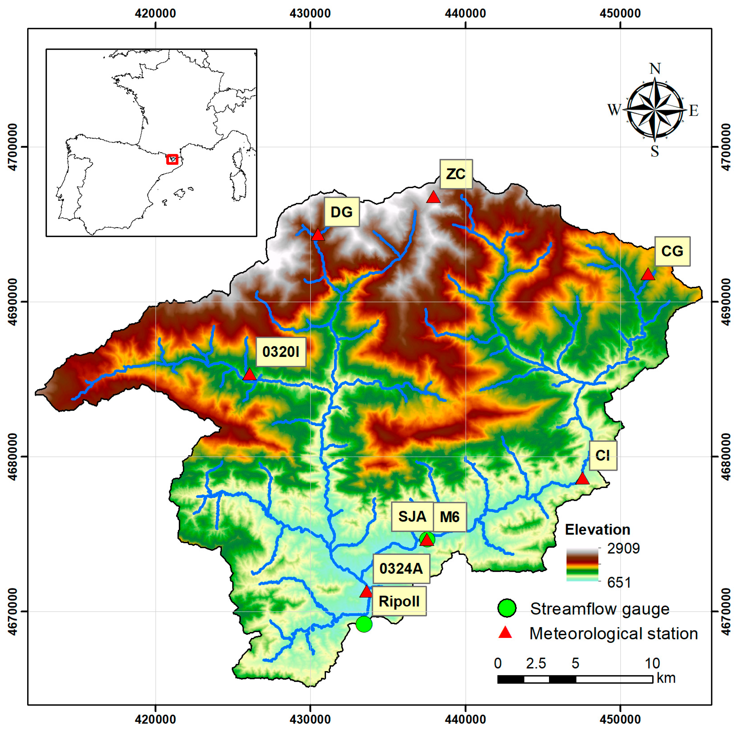
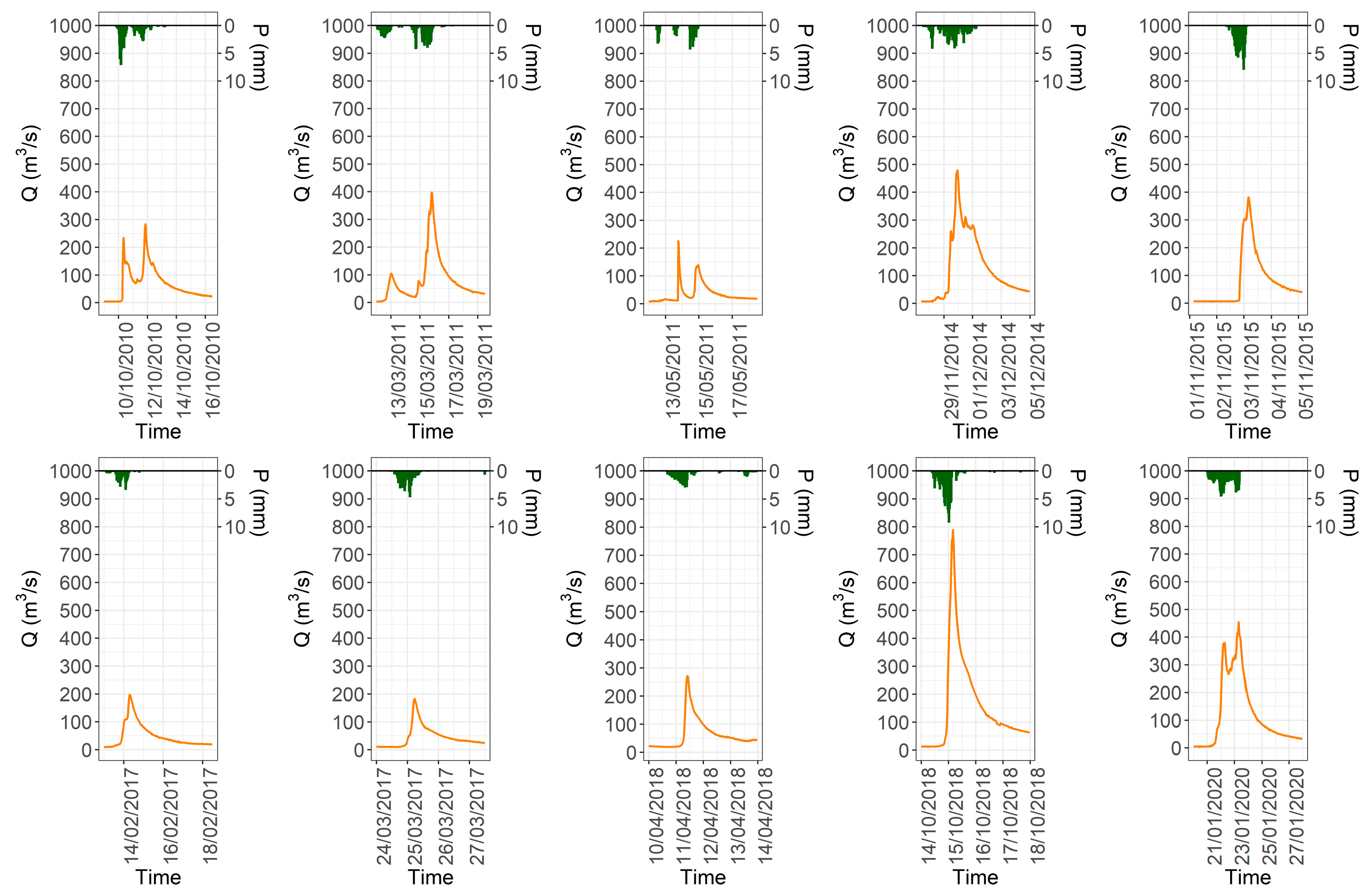
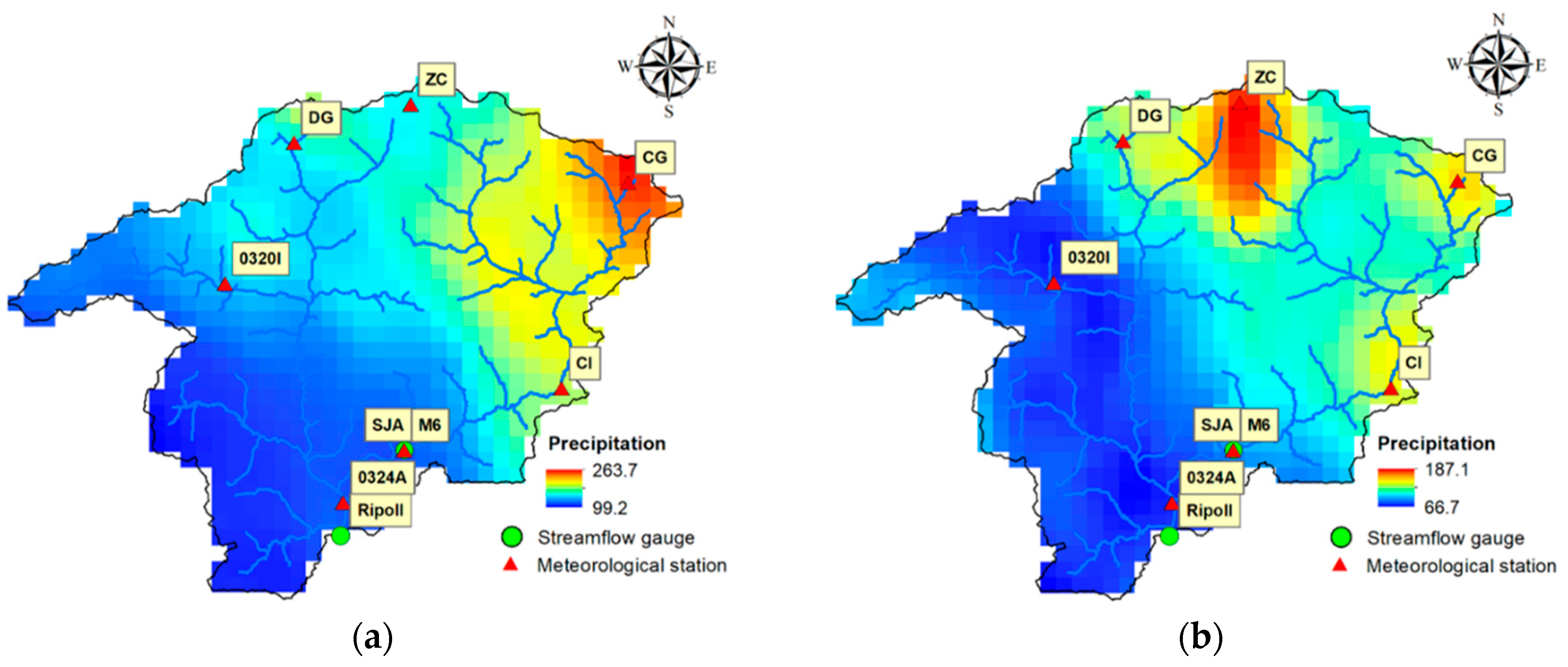
2.2. Data and Study Area

Data belonging to the Upper Ter Catchment located in Catalonia, north-eastern Spain, was employed in this research (Figure 1). The catchment is delimited by the outlet point in the small town of Ripoll. It encompasses an area of 737.73 (km²). The mean slope of the catchment and length of the mainstream are approximately 45% and 45.64 (km), respectively. Considering these characteristics, an approximation of the time of concentration given by Giandotti [36] is 7.9 (hours) (methodology applicable according to the catchment size [37]). The significant mean slope and intense rainfall may generate flash floods in the area. In fact, from 1982 to 2007, 82% of floods in Catalonia were flash floods [38]. The elevation difference is 2258 (m) (the lowest point at 651 (masl)), with the northern part of the catchment belonging to the Pyrenees. However, snow cover plays a minor role in the catchment system [39,40]. The digital terrain model of Figure 1 was drawn employing the public information of the Cartographic and Geological Institute of Catalonia [41].

According to INUNCAT [42], the municipality of Ripoll is cataloged as a high-risk region due to floods and, therefore, one of the regions with the highest levels of precipitation. These are mainly related to advection processes from the east and low-pressure nuclei that cross the region and are activated after reaching the Mediterranean Sea [43].

30-min precipitation (mm) and streamflow (m³/s) data are used to obtain the respective features in the RF model of this research. These data come from seven meteorological stations (Figure 1). Two of them belong to the Meteorological State Agency (AEMET, according to its acronym in Spanish): Planoles (0320I) and Ripoll (0324A) (their codes are between brackets). Five belong to the Meteorological Service of Catalonia (Meteocat, according to its acronym in Catalan): Molló-Fabert (CG), Sant Joan de les Abadesses (M6), Ulldeter (ZC), Sant Pau de Segúries (CI), and Núria (DG). Streamflow data is obtained from two stations: Sant Joan de les Abadesses (SJA) and Ripoll, whose information is managed by the Catalan Water Agency (ACA, according to its acronym in Catalan). The RF model of this research employs high streamflow events for training. In particular, those with peak flow greater than 180 m³/s (roughly the 1.5-year return period, 188.4 m³/s [44]), in the period between January 2010 and December 2022, resulting in 10 high streamflow events. The threshold value was selected because it has been related to bankfull flow [45,46,47]. There are missing values in the data set, which were omitted in this study. In addition, the period from January 2010 to September 2011, which is missing in the ZC station, is covered by a former station Z4, which used to be located in the vicinity (500 m from ZC). The hydrographs of the events employed and the respective mean precipitation of the catchment are depicted in Figure 2. The highest event (10/2018) is known as the Leslie storm.

2.3. The ML Predictive Model Based on Random Forest

Random Forests (RFs) are based on a—typically—big number of simple models based on decision trees. The decision tree is a technique that employs recursive partitioning to divide the data by searching homogeneous groups or nodes (e.g., small differences between the values and their mean inside the node) [9]. Initially, the data is gathered in a single node (root), which is split into daughter nodes (branches) using a criterion based on a variable (e.g., $x_j>s$, being $s$ a split value) [29]. This procedure continues until a criterion is reached such as the maximum number of values inside a node. The final nodes are usually denominated leaf nodes.

RF was introduced by Breiman [31] as an ensemble of decision trees, which are created using bagging (bootstrap aggregating) and random feature selection at each split. Bagging is a resampling method that generates new training sets by randomly extracting certain samples from the data set, and may replace them by repeating others. The samples taken out from the data set are called out-of-bag (OOB) data [48]. The proportions of samples in and out of the data set are approximately 63% and 37%, respectively [49]. The decision trees are created using the training sets generated by the bagging technique, and the variable for the partition is selected from a random set at each split. In regression models, the final prediction is given by the mean of the predictions of all decision trees. At the same time, the prediction of a single tree is given by the mean of a specific node. RF is a robust method employed broadly for streamflow prediction [16,50]. It is not usually affected by overfitting, and even the default parameters generally produce acceptable results [51,52]. This study employs the ranger package (version 0.16.0) of the R language [53] to train the RF models.

2.4. Feature Selection

The RF algorithm may present a moderate degradation of its accuracy due to the random addition of uninformative variables to each split while the trees are growing [48]. Consequently, a feature selection procedure is applied in this research to avoid this issue and have a reduced set of features, which can be suitable for evaluation. In addition, a reduced set of features decreases the computational cost for the different feature interpretation analyses. The feature selection procedure proposed by López-Chacón et al. [44] was followed in this research. They considered a set of initial features to train a first RF model. Based on that, the feature importance is estimated using the MDA analysis (Section 3.2). Then, several models are trained, removing a feature each time, starting from the least important one. The average root mean square error (RMSE) is computed from a cross-validation procedure (Section 2.5) for every combination of features. The selected set of features is the one that produces the minimum average RMSE.

Table 1. Selected set of features for the streamflow prediction model.

Station	Inputs	Output
Ripoll	$Qt\_h; h\in \{3, 3.5, 4, 4.5, 5, 20\}$	$Qt$
SJA	$Qt\_h; h\in \{3, 3.5, 4\}$
CI	$AccuT\_t\_3; T\in \left\{3, 4, 5, 6, 7, 8, 9, 10, 11, 12, 30, 36, 42 \right\}$    $AccuT\_t\_4; T\in \left\{3, 30\right\}$
CG	$AccuT\_t\_3; T\in \left\{30, 36, 42\right\}$    $AccuT\_t\_4; T\in \left\{36\right\}$
DG	$AccuT\_t\_3; T\in \left\{24, 36\right\}$
M6	$AccuT\_t\_3;T\in \left\{3, 4, 36\right\}$
ZC	$AccuT\_t\_3;T\in \left\{18, 24\right\}$

shows the selected set of features, while

Table A1. Initial set of features for the prediction model. These variables are taken from all the stations considered in the study.

Inputs		Output
$Pt\_h; h\in [3,7]$   $AccuT\_t\_k; T\in${3, 4, 5, 6, 7, 8, 9, 10, 11, 12, 18, 24, 30, 36, 42, 48}; k ∈ {3, 4, 5}		$Qt$
Qt_h; h ∈ {3, 3.5, 4, 4.5, 5, 5.5, 6, 6.5, 7, 7.5, 8, 8.5, 9, 9.5, 10, 10.5, 11, 11.5, 12, 13, 14, 15, 16, 17, 18, 19, 20, 21, 22, 23, 24, 25, 26, 27, 28, 29, 30, 31, 32, 33, 34, 35, 36}	${Gradient}_{Qt\_3,Qt\_4}$

and Figure A1 show the initial set of features (with data from every station) and the variation in average RMSE according to the number of variables, respectively. The initial set of features comprises 458 features, from which 35 features were selected. Features from 0320I and 0324A stations are not taken into account after the selection procedure. In the feature selection process, the RF models employed with every set of variables use the most common parameters in the literature (the number of random features is the total number of features divided by 3 and 500 trees) [52]. After the feature selection process is finished, the hyperparameter selection takes place, searching for a suitable combination of parameters for the model (Section 2.5). The streamflow prediction model employs precipitation and streamflow data as inputs. $Pt\_h$ refers to the hourly precipitation at time $t-h$, being $t$ the prediction time. $AccuT\_t\_k$ is the accumulated precipitation of $T$ hours at $t-k$. $Qt$ is the observed streamflow at the prediction time. $h$ and $k$ are given in hours. ${Gradient}_{Qt\_3,Qt\_4}$ is the difference between $Qt\_3$ and $Qt\_4$ in Ripoll station. The prediction horizon employed to train the streamflow prediction model is three hours ahead.

2.5. Hyperparameter Tuning

This research considered two hyperparameters for tuning: the number of trees ($ntree$) and the number of random variables at each split ($mtry$). Scornet [54] mentions that the higher the $ntree$ (according to the computational power), the better the performance of the model. Probst and Boulesteix [55] reached similar conclusions, but they outlined that the highest improvement of the model is given in the first 100 trees. Nonetheless, this number might be influenced by hypermeters such as a small $mtry$, while trees are growing will generate significantly different trees, and therefore, more trees will be needed. Regarding a streamflow prediction model, Contreras et al. [56] stated that the $ntree$ was the most influential hyperparameter according to their results. On the other hand, it has been found that $mtry$ has a significant effect on the RF model performance [57]. Even Probst et al. [52] and Van Rijn and Hutter [58] show this hyperparameter as the most influential in their respective research. Other studies have also employed these hyperparameters in a tuning procedure [16,59]. The hyperparameters were determined using the minimum averaged RMSE in cross-validation and grid search procedures, whose set of values is shown in

Table 2. Set of hyperparameters employed in the tuning procedure of the streamflow prediction model.

Set of Hyperparameters	Selected Combination
$ntree=\left\{400, 500, 600, 700\right\}; mtry=\{8, 10, 12, 14, 16\}$	$ntree=500; mtry=12$

, as well as the selected combination of them. The cross-validation method employed is a prequential analysis [60], which is explained in detail in Appendix A.

3. Model Interpretation Methods

3.1. Mean Decrease Impurity

In regression models, the impurity in a given node ($k$) is measured by the residual sum of squares ($RSS$) with regard to the mean of the node (1) [61]. A specific criterion based on a feature $j$ splits the node, generating a decrease in node impurity related to this feature (${DI}_{k,j}$) (2):

$${RSS}_k=\sum _{iϵk}{\left(y_i-{\overline{y}}_k\right)}^2$$

(1)

$${DI}_{k,j}={RSS}_k-{RSS}_p$$

(2)

where $y_i$ is an observation inside the node k, and ${\overline{y}}_k$ is the mean value of all observations of node k. The ${DI}_{k,j}$ is given by the difference between the impurity of the node before splitting (${RSS}_k$) and the combined impurity of the partitions after splitting (${RSS}_p$) [9]. The combined impurity of partitions is given by the sum of impurities of the left and right daughter nodes (following the same approach as in (1) for both nodes). Finally, the decrease in impurity related to a feature in every tree is summed and divided by the number of trees to obtain the MDI. If a split criterion based on a feature $j$ generates nodes with considerably low impurity (small differences between the values and the mean inside the node), the MDI related to that feature will be high, as well as its importance.

3.2. Mean Decrease Accuracy

To compute the MDA related to a feature:

• The error of the OOB values for a tree is computed based on the mean squared error (MSE).
• The feature $j$ is permuted in the same group of OOB values, and the MSE is calculated.
• The difference between the MSE of the permuted and original set of OOB values is summed and divided by the number of trees (3) [30,62]:

  $${MDA}_j={\displaystyle \frac{1}{ntree}}\sum _{t=1}^{ntree}({MSEP}_{t,j}-{MSE}_{t,j})$$

  (3)

  where ${MSEP}_{t,j}$ and ${MSE}_{t,j}$ correspond to the MSE of the OOB values with feature $j$ permuted and not permuted, respectively. $t$ is the number of trees. The higher ${MDA}_j$, the higher the importance of feature $j$. Both MDA and MDI are computed using ranger package.

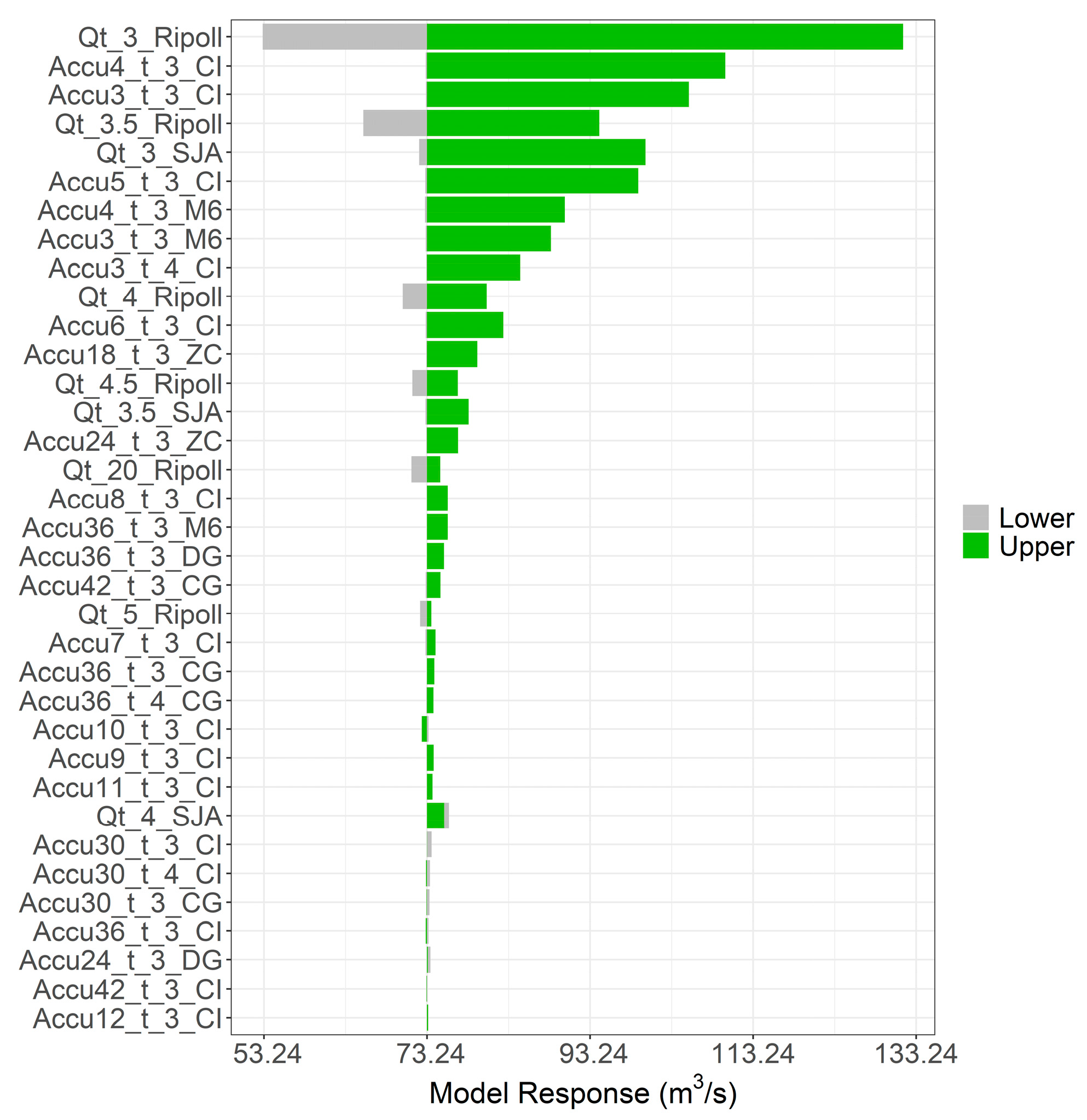
3.3. Tornado Diagrams

Tornado diagrams are generally employed for sensitivity analysis [32,63]. The center of the tornado diagrams presented in this study shows the response of the RF model when all the features correspond to their mean. In addition, the diagrams show how the model responds when all the features are kept at their mean while the variable whose impact on the model is studied varies between its minimum and maximum values. This study employs the package tornado (version 0.1.3) [64] to obtain these diagrams.

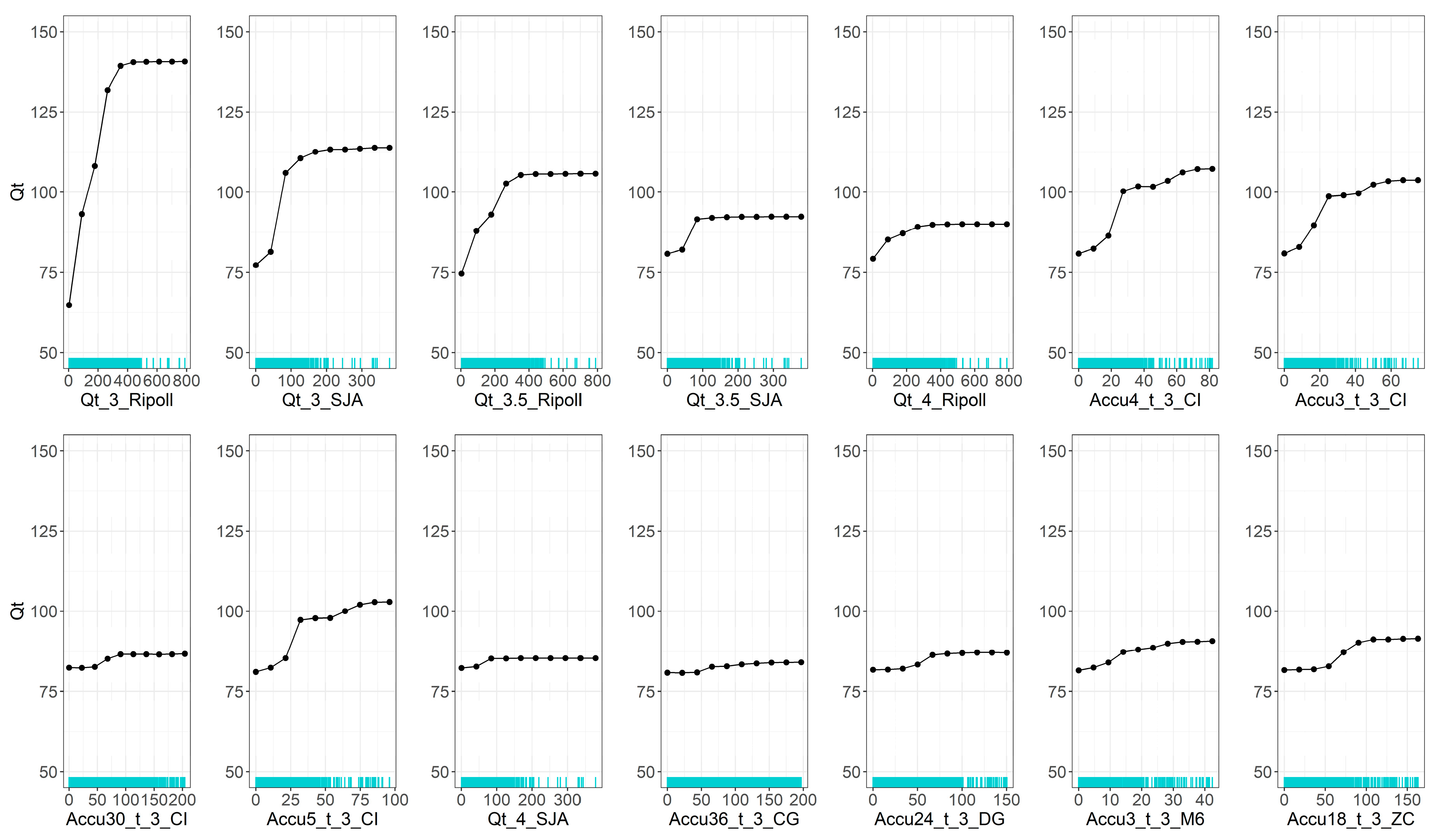
3.4. Partial Dependence Plots

A partial dependence plot explores the marginal effect of a feature on the model’s response [33]. The plot is based on function $\widehat{f}\left(x_p\right)$ (4), which computes the average effect of a value $p$ of the feature $x$. $X_{i,C}$ represents the set of other features, which are not evaluated and preserve their respective values in every instance. Therefore, to evaluate the effect of the value $p$ of the feature $x$, all the values of $x$ are replaced by $p$ in every instance, and the average response of the model is obtained [65].

$$\widehat{f}(x_p)={\displaystyle \frac{1}{n}}\sum _{i=1}^{n}f(x_p,X_{i,C})$$

(4)

where $n$ is the number of instances of the data set. A grid of $p$ values are selected to compute the partial dependence following the aforementioned procedure to create the curve of the plot.

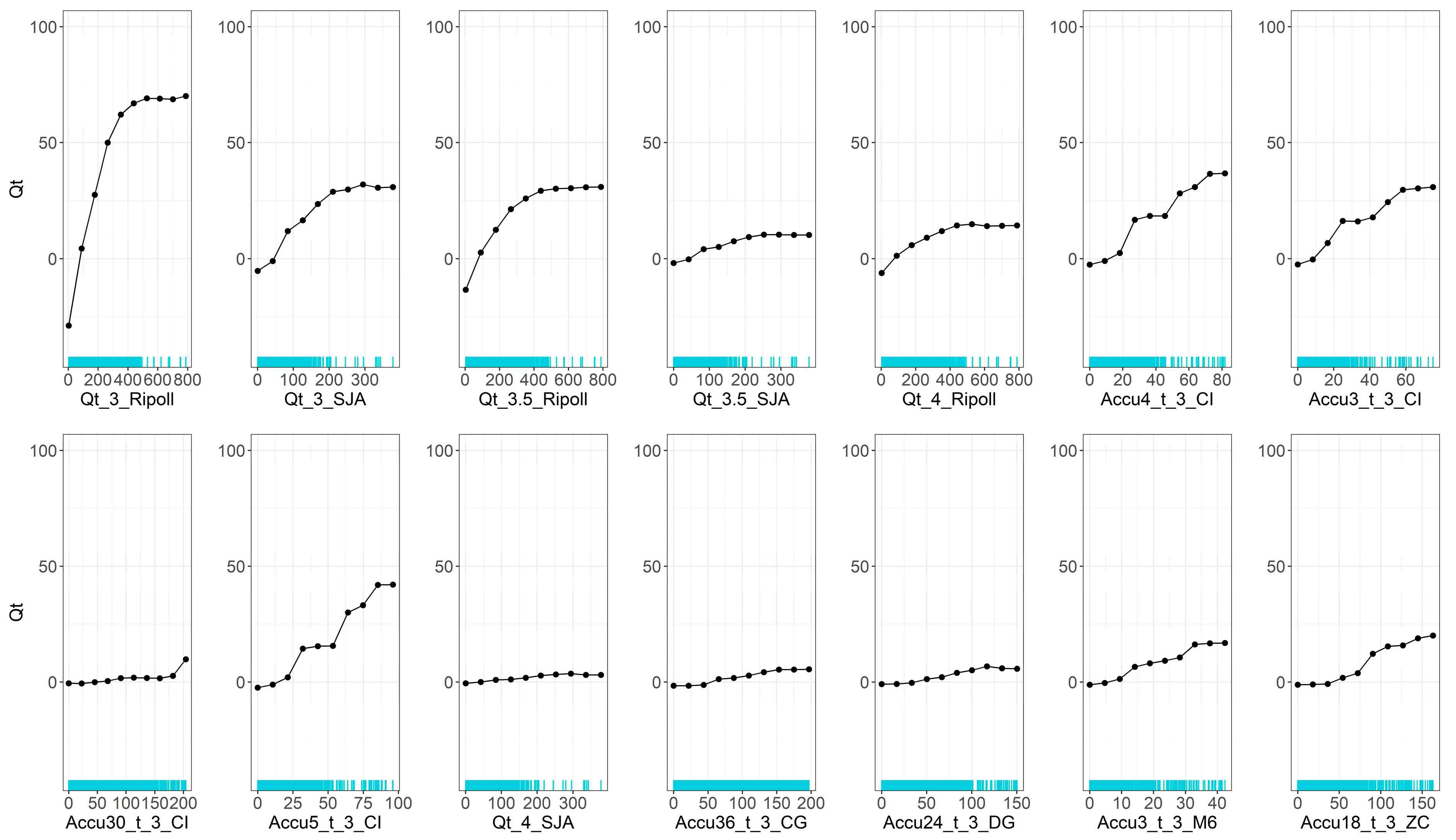
3.5. Accumulated Local Effect

The PDP analysis might produce an inaccurate description of the effect of a feature because the procedure does not resemble reality if there are correlated features in the model [15]. The PDP ignores this correlation by establishing one single value $p$ for $x$ while a correlated feature varies over its whole spectrum, instead of varying over a correlated range of values. ALE [34] was formulated to tackle this drawback in PDPs. It combines the marginal plots (M-plots) with differences in predictions to obtain the effect or influence of a feature. ALE evaluates the effect of the feature $x$ considering realistic values of other features (conditional distribution) and avoids possible mixing effects of other correlated features (the main reason why it employs differences instead of averages) [65]. The procedure starts by creating intervals of the feature, whose effect on the output is to be evaluated. Grid points ($z_{w,j}$) define the intervals. The number of instances inside the interval is given by $n_j\left(w\right)$, where $w$ and $j$ refer to the number of intervals and the feature under evaluation, respectively. Assuming that the feature $x$ needs to be evaluated, the uncentered ALE (${\widehat{g}}_{j,ALE}\left(x\right)$) is computed based on (5):

$${\widehat{g}}_{j,ALE}(x)=\sum _{l=1}^{w_j\left(x\right)}{\displaystyle \frac{1}{n_j\left(w\right)}}\sum _{i:x_{i,j}\in (z_{w-1,j},z_{w,j}]}\left\{f\left(z_{w,j},x_{i,\backslash j}\right)-f\left(z_{w-1,j},x_{i,\backslash j}\right)\right\}$$

(5)

where $(z_{w-1,j},z_{w,j}]$ are the limits of a given interval, $f$ refers to the model (in this case the RF model), and $x_{i,\backslash j}$ corresponds to the rest of the features inside the interval. Equation (5) implies that for obtaining the uncentered ALE of a feature value that belongs to a certain interval of values, the sum of the effects of previous intervals will be calculated. ${\widehat{g}}_{j,ALE}\left(x\right)$ is later centered by ${\widehat{f}}_{j,ALE}\left(x\right)$ obtaining the main ALE expression (6):

$${\widehat{f}}_{j,ALE}\left(x\right)={\widehat{g}}_{j,ALE}\left(x\right)-{\displaystyle \frac{1}{n}}\sum _{w=1}^W{n}_j\left(w\right){\widehat{g}}_{j,ALE}\left(z_{w,j}\right)$$

(6)

where $W$ is the total number of intervals. ALE values can be understood as the impact of a specific value of a feature regarding the mean prediction of the model [65]. PDP and ALE are computed using iml (Interpretable Machine Learning) package (version 0.11.3) of R language [66].

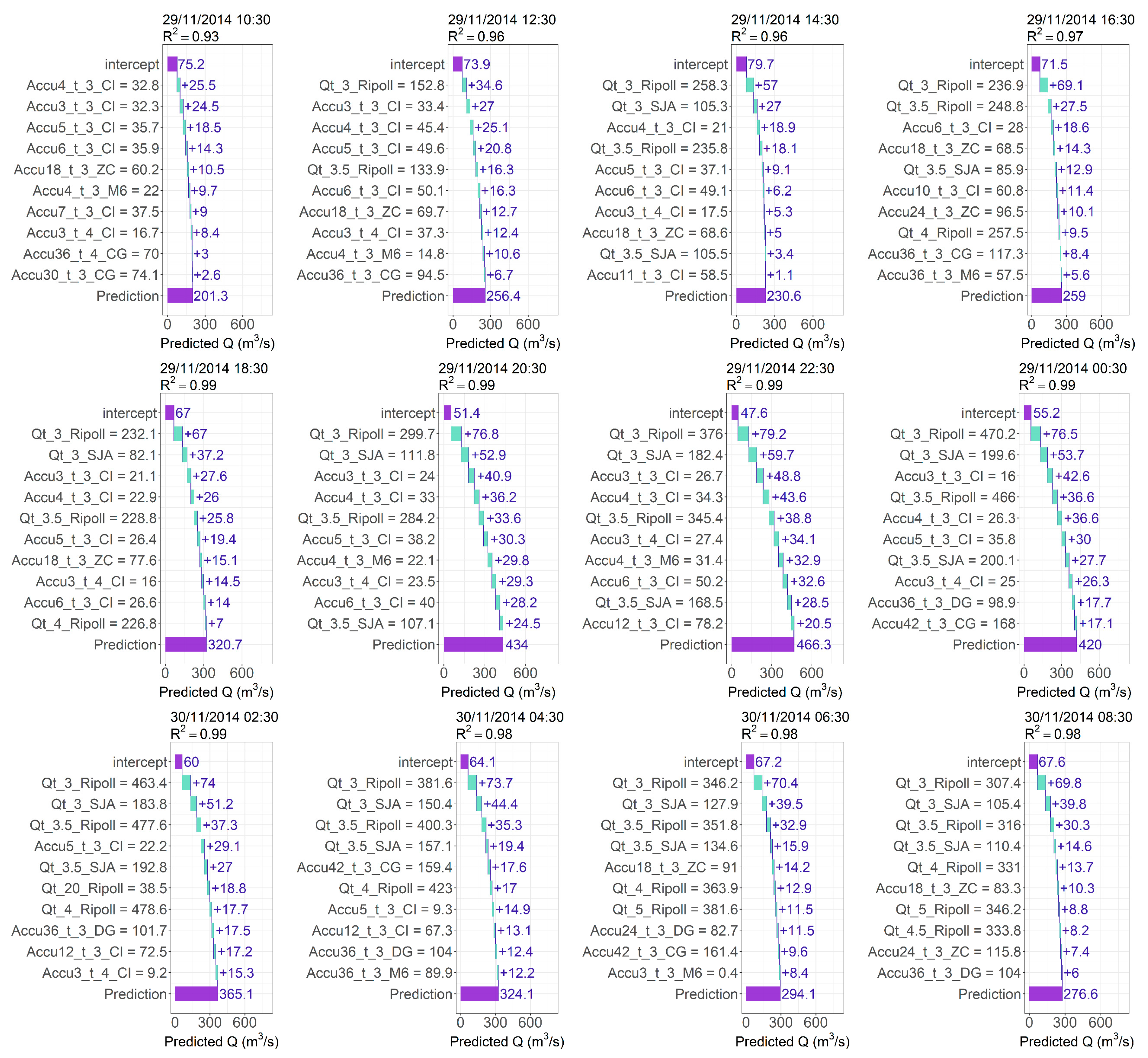
3.6. Local Interpretable Model-Agnostic Explanations

Ribeiro et al. [35] proposed LIME to create a local explanation model, where the feature effect in a single prediction can be interpreted. The inspiration of this method is based on obtaining a simpler model than the ML model to explain the effect of the features on a single prediction. The explanation ($\xi \left(x\right)$) is given by (7) as follows:

$$\xi \left(x\right)={argmin}_{g\in G}L\left(f,g,{\pi }_x\right)+\Omega \left(g\right)$$

(7)

where the objective is to minimize the loss function $L\left(f,g,{\pi }_x\right)$ (weighted residual sum of squares) that measures the proximity of the explanation model ($g$) to the prediction of the ML model ($f$) (RF in this case). $G$ is a set of possible explanation models. Usually, explanation models do not use the whole set of features ($x$) in an instance but a simplified version ($x^{\prime }$). ${\pi }_x$ is a kernel function that depends on the distance between an instance of interest and the rest of the instances, and a width to define how large the set of proximate instances will be. Finally, $\Omega \left(g\right)$ refers to a penalty due to the complexity of the explanation model (e.g., how many variables it has). In practice, the user of the method must establish the number of variables to be used in $g$ and the distance measurement method [15]. The distance method used in this research is the Euclidean. One of the most popular explanation models is Lasso (the least absolute shrinkage and selection operator, also used in this research) [65].

This method has some sources of uncertainty: the variables selected to explain a single prediction, the variation in data taken into account given by the proximity threshold and other parameters (such as the distance method), and the application of the model with the same parameters to other predictions [67]. In addition, in regression models, the method usually divides the variables into bins to relate the explanation to a range instead of a single sample [68]. The kernel width and the number of bins are LIME parameters tuned in this research by searching for the highest mean determination coefficient ($R^2$) over 24 individual instances corresponding to the two highest events. LIME analysis is computed using the lime package version 0.5.3 of R language [69].

3.7. Shapley Values

Shapley [70] proposed the Shapley values as a method to estimate the contribution of each player to a final payout. This methodology can also be applied to evaluate a feature effect in a specific instance [71]. However, to evaluate this, all different coalitions must be considered (combinations of features). Therefore, Shapley values compute the average of all marginal contributions of a feature in a specific instance over all possible coalitions. Mathematically, the Shapley value of a feature $j$ of an instance is given by (8):

$${\varphi }_j=\sum _{S\subseteq F\backslash \left\{j\right\}}{\displaystyle \frac{\left|S\right|!\left(\left|F\right|-\left|S\right|-1\right)!}{\left|F\right|!}}\left[f\left(x_{S\cup \left\{j\right\}}\right)-f\left(x_S\right)\right]$$

(8)

where $S$ is a subset of features included in the whole set of features $F$ where the feature $j$ is marginalized. $\left|F\right|$ and $\left|S\right|$ refer to the number of features inside these sets. $f\left(x_{S\cup \left\{j\right\}}\right)$ and $f\left(x_S\right)$ are the predictions of the model with and without the actual value of the feature $j$ of the instance, respectively. It can be computationally unbearable to calculate Equation (8) if the model comprises many features and, therefore, different combinations of them. In that sense, other approaches like SHAP have emerged to estimate the Shapley values (Section 3.8). The Shapley value can be interpreted as the contribution of a feature to the difference between the prediction corresponding to an instance (which is evaluated) and the mean prediction [65].

3.8. Shapley Additive Explanations (SHAP)

Explanation methods for specific predictions such as LIME (Section 3.6) employ simplified models ($g$) to explain in a simple way the effect of a feature in a given prediction. As was previously mentioned, $g$ may use fewer features ($x^{\prime }$) than the original set of features ($x$) to describe the prediction. However, the goal is to obtain a function $g\left(x^{\prime }\right)$ that obtains similar results to the original model $f\left(x\right)$, $g\left(x^{\prime }\right)\approx f\left(x\right)$. In this sense, $g\left(x^{\prime }\right)$ follows an additive feature attribution form (9) [72]:

$$g(x^{\prime })={\varphi }_0+\sum _{j=1}^M{\varphi }_j{x^{\prime }}_j$$

(9)

where $M$ is the number of simplified features $x^{\prime }$, ${\varphi }_0$ corresponds to a first approximation if the values of the features are not known, this value is generally assumed as the mean prediction of training. Three properties are desirable for the solution (${\varphi }_j$) of Equation (9): local accuracy, missingness, and consistency [73]. Local accuracy refers to the fact that $g\left(x^{\prime }\right)$ and $f\left(x\right)$ obtain similar results in a given instance. Missingness implies that for a feature that was excluded from (9) (${x^{\prime }}_j=0$), its effect must be null (${\varphi }_j=0$). Finally, consistency implies that if the value of a feature increases or remains the same, the effect of this feature in the prediction cannot decrease. Lundberg and Lee [18] stated that only one model $g$ can be applied to explain the feature effects that fulfill the three properties and proposed SHAP, another method to obtain approximations to the Shapley values employing fewer evaluations of the model and, therefore, lower computational cost than (8). They noticed that LIME (Section 3.6) corresponded to an additive feature attribution form (9). Therefore, the coefficients of $g$ in (7) correspond to the Shapley values if the three properties are fulfilled. To that aim, they proposed to set $\Omega \left(g\right)$ as 0 and ${\pi }_x$ given by (10):

$${\pi }_x(z^{\prime })={\displaystyle \frac{M-1}{\left(M choose \left|z^{\prime }\right|\right)\left|z^{\prime }\right|\left(M-\left|z^{\prime }\right|\right)}}$$

(10)

where $z^{\prime }$ comprises a fraction of $x^{\prime }$ values (a coalition of values in $x^{\prime }$). $\left|z^{\prime }\right|$ is the number of features in $z^{\prime }$. $M choose \left|z^{\prime }\right|$ is the number of coalitions of size $\left|z^{\prime }\right|$. SHAP values are the components of the linear regression (9) that assign a change over the mean prediction ${\varphi }_0$ to every feature regarding the predicted value. This research employs treeshap package (version 0.3.1) of R language, which is based on the work of Lundberg et al. [72] to compute SHAP values in tree-based models. SHAP is also employed for a general analysis in this research by computing the mean absolute SHAP value of every feature of all single predictions.

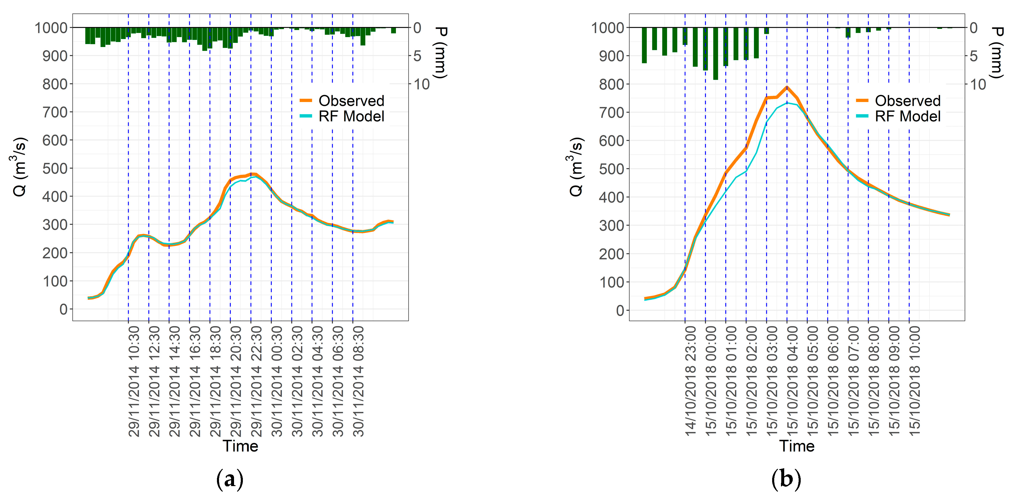
4. Results and Discussion

The different feature interpretation analyses were applied to a model trained as described in Section 2. In particular, the training set (10 events) was considered to evaluate the feature interpretation analyses. This is based on two criteria. First, some methodologies such as the MDA and MDI are necessarily computed while the RF model is being trained. Second, according to Molnar [65], using the training set to evaluate the feature effect on a model is related to knowing how much the model depends on a feature to produce a prediction. This is associated with the goal of this research, which is to find hydrological insights into how the model works. However, to verify that the feature interpretation analysis makes sense and to associate the results from a hydrological perspective, it is necessary to verify the model accuracy. Therefore, the results of the cross-validation procedure for the selected parameters ($ntree=500;mtry=12$) are shown in

Table 3. Error metrics in cross-validation procedure for the selected combination of parameters of the RF model.

Error Metric	Fold 1	Fold 2	Fold 3	Fold 4	Fold 5	Average
RMSE (m3/s)	21.06	10.29	17.85	61.42	50.66	32.26
PBIAS (%)	11.41	5.06	0.47	−14.52	−6.91	−0.90
NSE	0.91	0.94	0.86	0.78	0.87	0.87

where the well-known metrics percentage bias (PBIAS) and Nash-Sutcliffe efficiency (NSE) (information on how to compute them can be found in López-Chacón et al. [44]) were calculated for every fold in addition to the RMSE as it was explained in Section 2.5. Moreover, the minimum, maximum, and mean observed streamflow values of testing folds are also depicted in

Table A2. Descriptive metrics of the testing folds of the cross-validation procedure.

Value	Fold 1	Fold 2	Fold 3	Fold 4	Fold 5
Minimum Observed (m3/s)	5.94	9.78	9.89	10.91	3.21
Maximum observed (m3/s)	380.85	196.12	271.02	788.51	788.51
Mean (m3/s)	59.97	46.82	54.11	109.22	129.91
Standard deviation (m3/s)	70.45	40.84	47.60	132.43	139.81

for a better understanding of the error metrics.

According to Moriasi et al. [74], a good predictive model on a monthly scale shall have an absolute PBIAS below 15% and NSE values higher than 0.65. Taking into account that the ML model of the current research is given on a smaller scale (half-hourly), the reference values for these metrics can even be loosened as explained by Kalin et al. [75]. Acceptable values of PBIAS and NSE are achieved in the five folds of the cross-validation procedure. However, the difference in metrics between the first three folds and the fourth one is related to the incorporation of the highest event (Leslie storm) in the testing set of that fold, whose magnitude has not been seen in training before. Even so, the RMSE value given in that fold (61.42 (m³/s)) is considerably smaller compared to the difference between maximum and minimum streamflow values (777.60 (m³/s)) and standard deviation (132.43 (m³/s)) (Table A2) in this fold. A similar situation is shown in the fifth fold. Based on the criteria proposed by Ritter and Muñoz-Carpena [76], which categorize performance as acceptable when the standard deviation is between 1.2 and 2.2 times the RMSE, all RMSE values obtained in Table 3 exhibit the RF model’s acceptable precision.

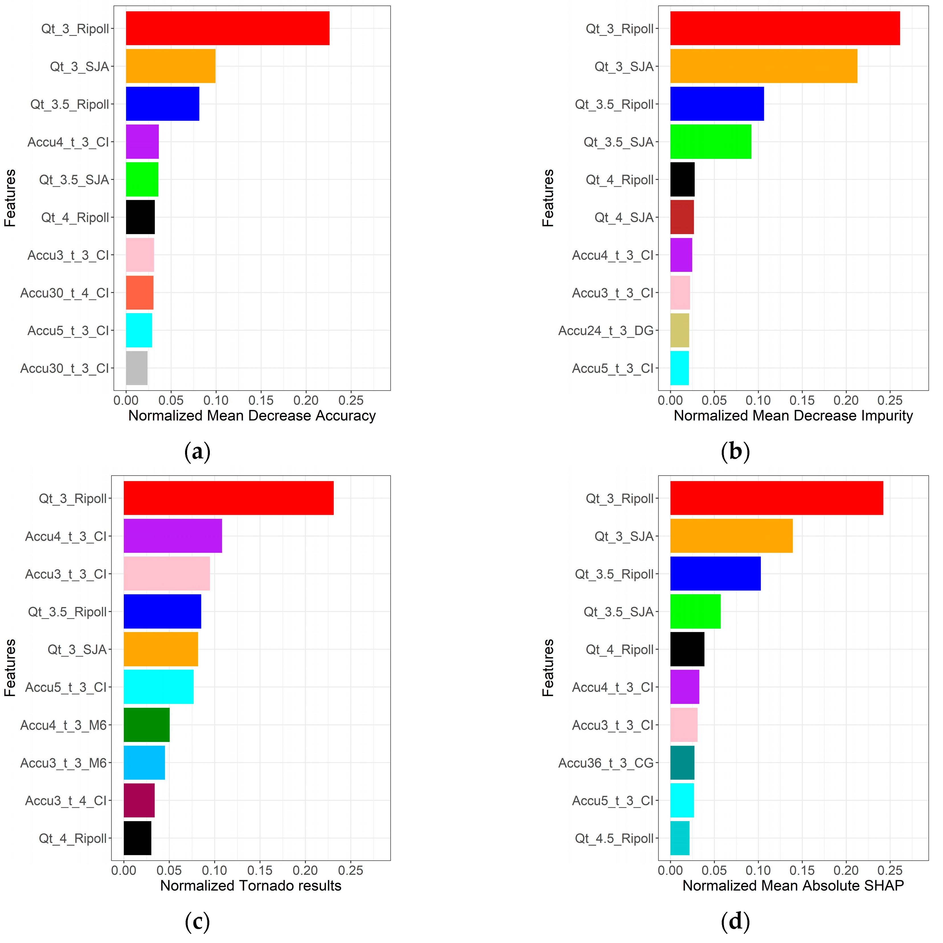
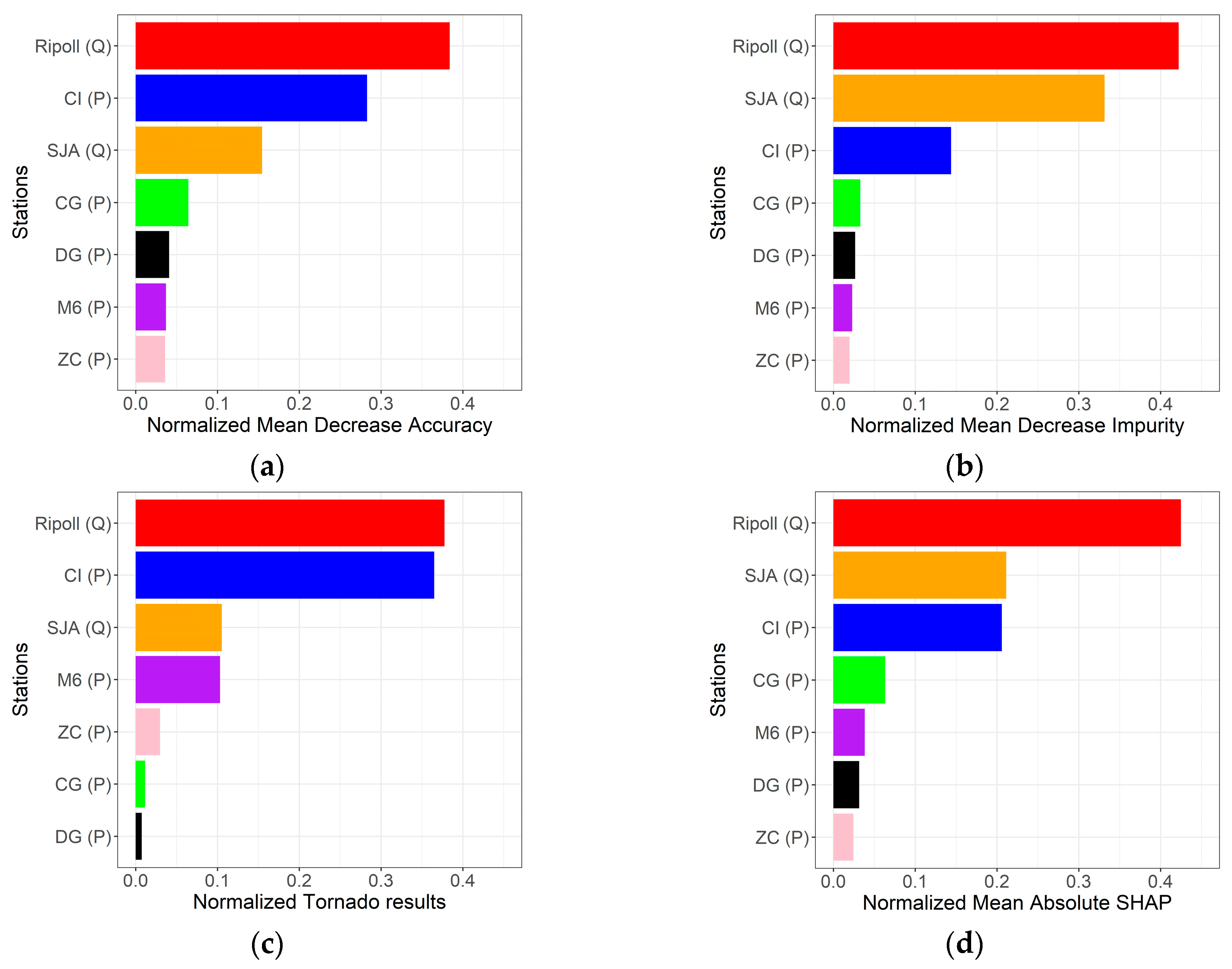
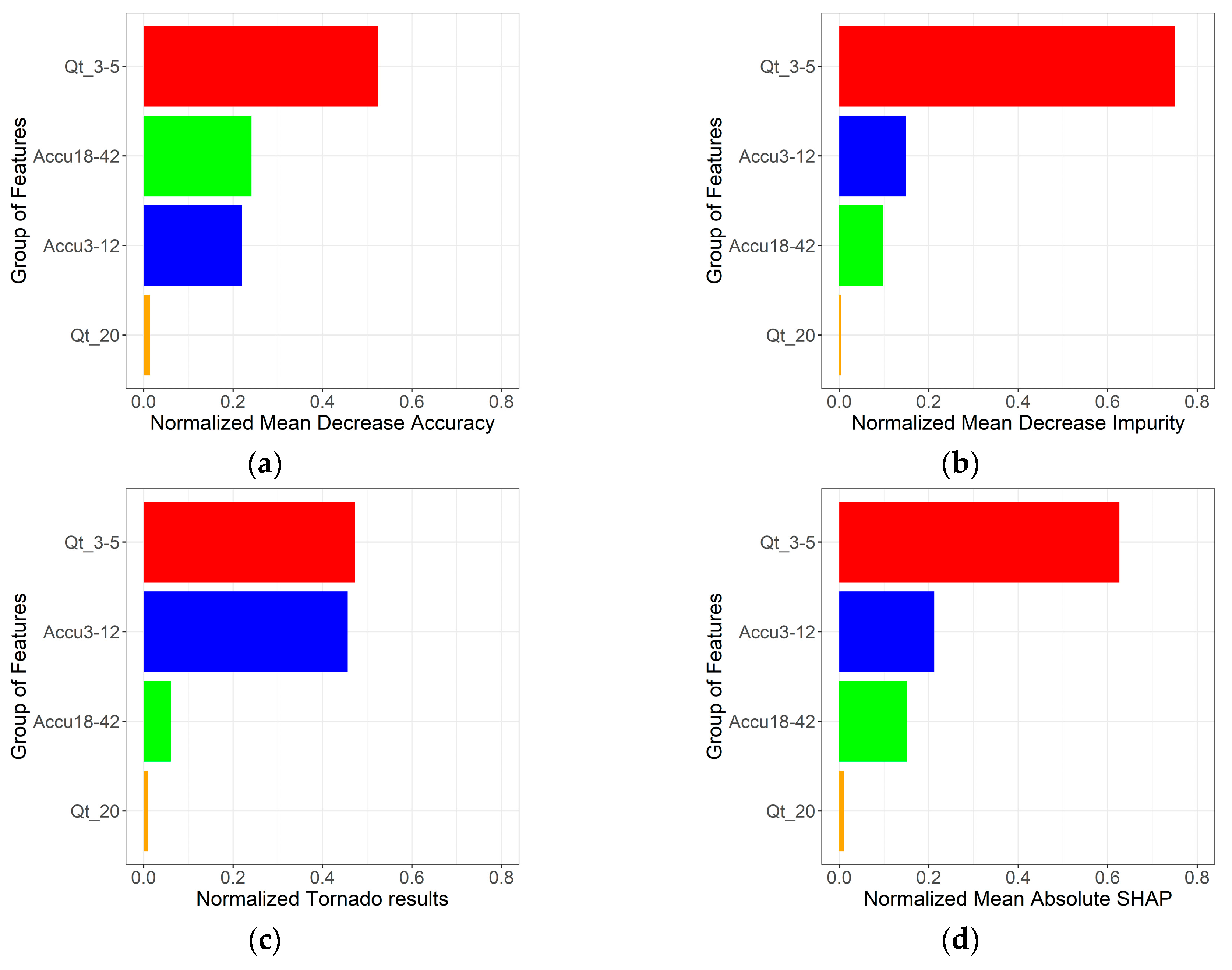
4.1. General Feature Importance Analysis

Normalized results are presented in Figure 3 to compare the MDA, MDI, Tornado analysis, and mean absolute SHAP, where MDA, MDI, and mean absolute SHAP values are normalized by dividing the actual value (resulting from the respective analysis) by the sum of the values for all the features. In the case of Tornado analysis, the value for a feature corresponds to the length of its variation range divided by the sum of the lengths of the ranges of all the features. The actual range of variation in the features due to the Tornado analysis is shown in Figure A3. Figure 3 shows the 10 features with the highest importance for every method for a straightforward comparison.

The streamflow at the outlet point three hours before the prediction time ($Qt\_3\_Ripoll$) is the most important feature in every method, accounting for more than 20% of the general importance compared to the rest of the features in every method. Even considering the significant temporal variation in streamflow in high events, shown in Figure 2, the antecedent streamflow still has the main importance. Consequently, this suggests that the biggest section of the predicted high streamflow hydrographs (the falling limb) is greatly influenced by this feature, which, together with others, can deliver an acceptable prediction. Seven features consistently rank among the top 10 across all methods, although the Tornado method shows a notably different order compared to the others. These discrepancies are related to the Tornado method measures how the output varies when a feature changes. However, it does not show how the variation in a feature affects the precision of the model output as in the case of the MDA and the MDI. Moreover, this method does not consider the interaction of a feature with others. In that sense, it is understandable that in the Tornado method, accumulated precipitation features are ranked higher compared to other methods, which acceptably implies a higher variation in the predicted streamflow when these features increase, for example. In general terms, MDA, MDI, and SHAP present similar results for the first 10 features. However, there are some differences such as the precipitation accumulated in 30 h, four hours from the prediction time in the CI station ($Accu30\_t\_4\_CI$), which is present in the first 10 features of the MDA analysis (Figure 3a) but not in the MDI and SHAP. Nevertheless, other features of accumulated precipitation over many hours ($Accu24\_t\_3\_DG$ and $Accu36\_t\_3\_CG$) are present in MDI and SHAP analysis in close positions. Nicodemus and Malley [77] stated that the MDI analysis may confer a higher importance to uncorrelated features because they were selected more often into the splits of the trees. On the other hand, Nicodemus et al. [78] argued that the correlated features (correlation > 0.80) may obtain a higher importance under the MDA analysis (streamflow features close to the time of prediction are substantially correlated to the prediction, >0.80 (Figure A4)). Despite the difference in these works, the present study shows that both analyses give similar results, mainly in the most important features, which are even supported by the SHAP results. This suggests that the general importance of the features is not strictly related to their correlation with the output. In other words, the RF model does not rely systematically more on features with high correlation with the output to make a prediction. Features such as $Accu36\_t\_3\_CG$ and $Accu18\_t\_3\_ZC$ (which are not part of the main 10 features according to the general importance analyses) have a correlation with the output of 0.79 and 0.80, respectively. On the other hand, $Accu4\_t\_3\_CI$ and $Accu3\_t\_3\_CI$ with a correlation of 0.62 and 0.58, respectively, are more important in the model and are consistently part of the main features in every method.

The results from the four analyses are grouped by the station they belong to, as shown in Figure 4. The streamflow values of the Ripoll station are the most relevant for the model according to every methodology, even reaching similar normalized importance values. The features of CI and SJA stations are in second and third place, depending on the method. In MDA and MDI analyses, there is a considerable difference in importance values between CI and SJA stations. However, this difference is significantly reduced in SHAP analysis. The features belonging to the CI station acquire notable importance in Tornado analysis, although considering the meaningful discrepancies with the other three methodologies, the results must be taken cautiously. Nonetheless, the most relevant precipitation values for the model come from the CI station, with a considerable difference from the rest of the precipitation stations. Not only do the majority of precipitation features come from the CI station, but also the most relevant. Therefore, the result of the Tornado method depicts the significant sensibility that the model has when only precipitation of this station varies, but it does not show the interaction with other features to contribute to the output as SHAP (for example), which may explain the high Tornado values of precipitation features of this station. On the other hand, the features from M6, DG, and ZC stations are the least relevant. At the same time, there is also a reduced group of features related to these stations. Even M6 station is closer to the outlet point than CI; the latter is considerably more relevant. This result suggests that the precipitation in the area where CI is located is the most influential for the streamflow at the prediction time and that the runoff produced in that area is considerable.

Accumulated precipitations of more than 18 h are considered from the most distant precipitation stations, ZC, CG, and DG. This suggests that the prediction model indirectly takes the distance into account and considers that to influence the output, several hours of precipitation have to be accumulated for these stations. According to Figure 5, where the feature importance is grouped by kinds of variables, 3 to 12 h of accumulated precipitation ($Accu3–12$) is the most relevant group of variables after the streamflow features (from three to five hours from the time of prediction ($Qt\_3–5$)) in the majority of methods. This result may be related to a lag time or time of concentration in the catchment. One possible approximation to the time of concentration (7.9 h) was given in Section 2.2. Considering the closer proximity to the outlet point from the CI station than the whole length of the mainstream, it is reasonable that a smaller time period is needed to influence the output from the CI station. This is reflected in the most important precipitation variable in every method, $Accu4\_t\_3\_CI$, which also indicates that the accumulated precipitation of a few hours is needed in that area to impact downstream. Previous humidity conditions are represented by an extended period of accumulated precipitation (mostly features of more than 18 h of accumulated precipitation ($Accu18–42$)) and its effect is close, although smaller, than the accumulated precipitation of fewer hours according to MDI and SHAP analysis. Nonetheless, it is even more significant than $Accu3–12$ in the MDA analysis. Figure 5 suggests that only streamflow values close to the time of prediction have a meaningful impact on the output of the model, but not streamflow values further in time ($Qt\_20$), which is also reflected in the selected features for the RF model (Section 2.4).

4.2. Partial Dependence Analysis

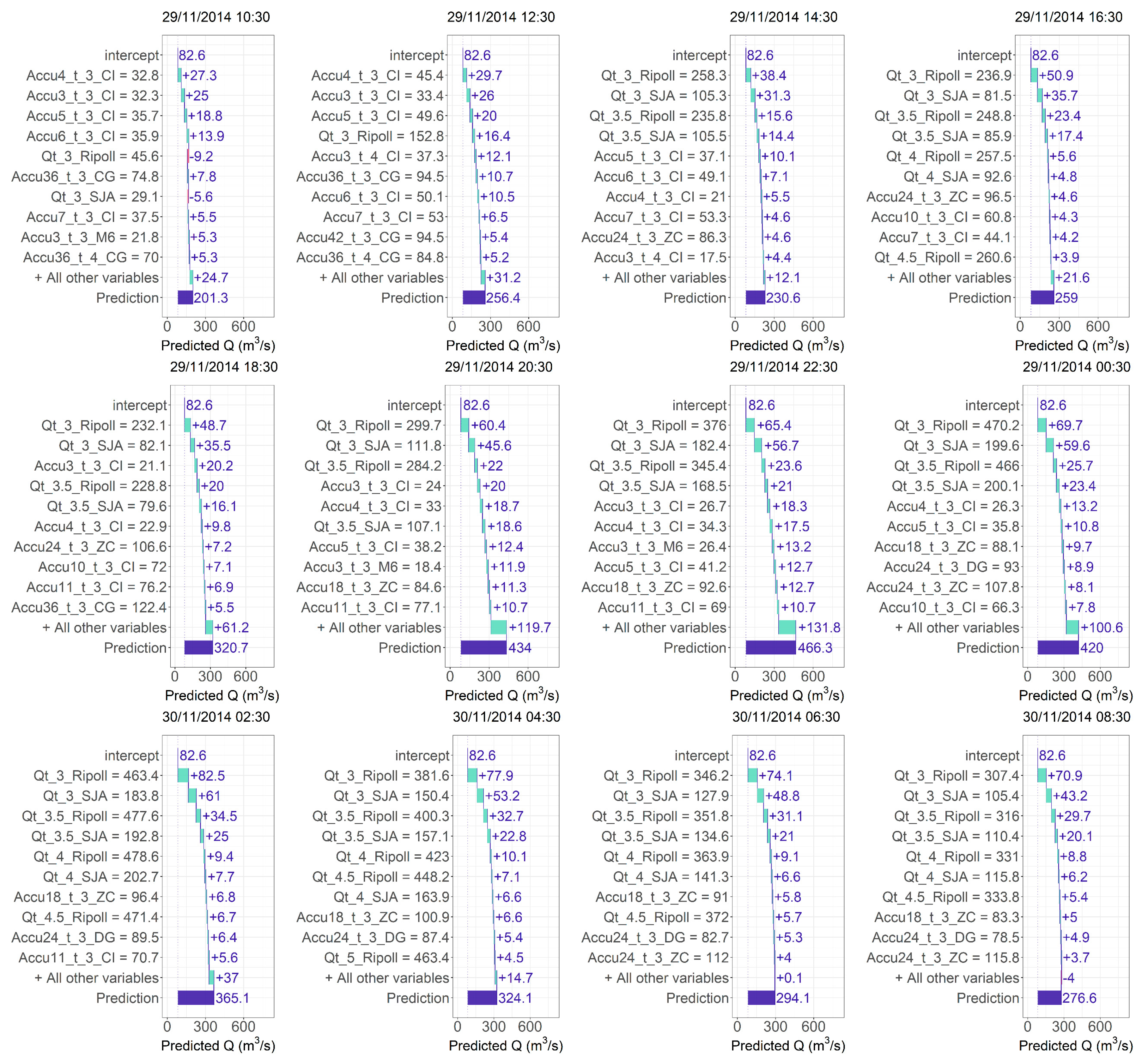
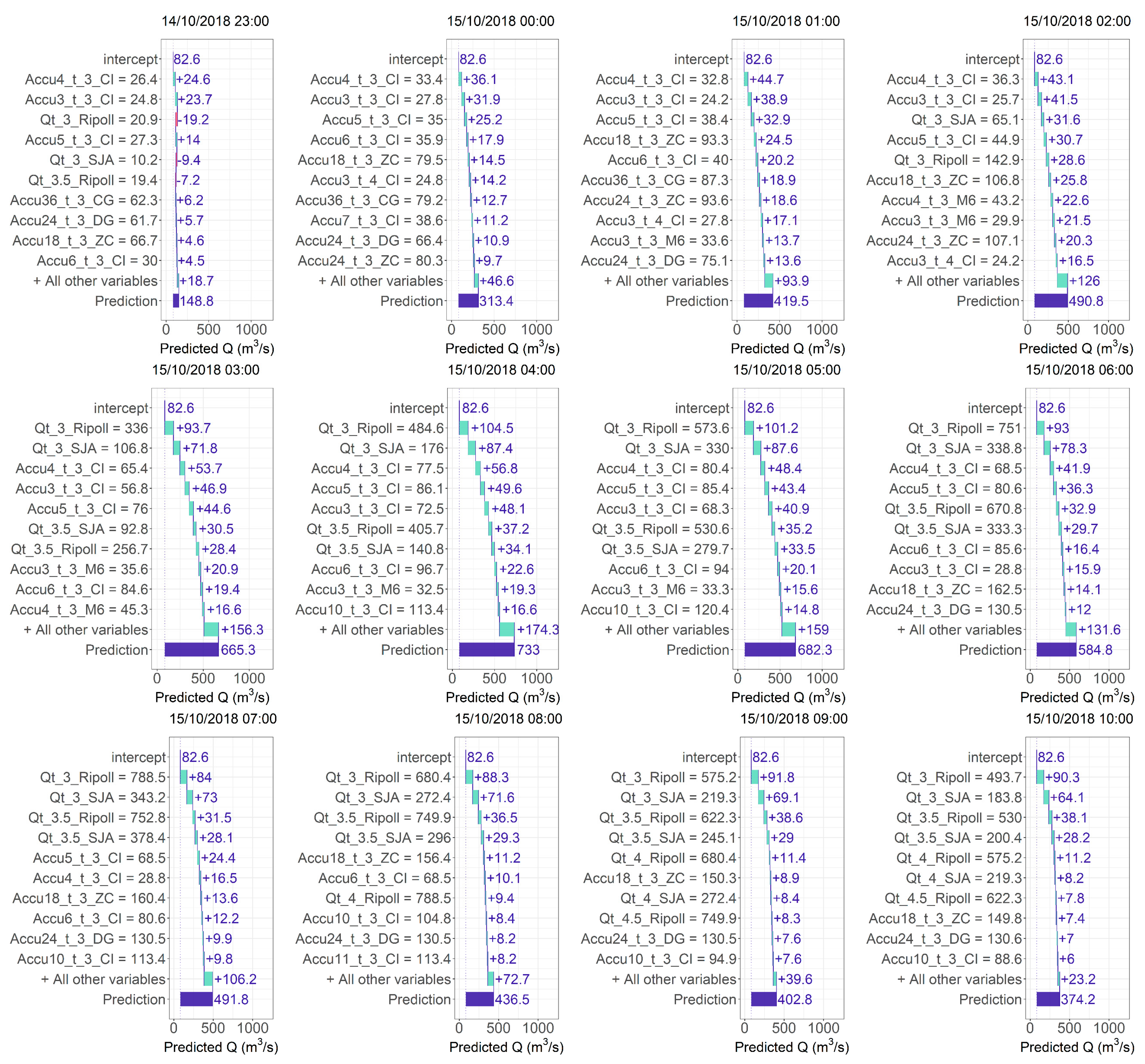
The effect of variation of the features on the output is evaluated by employing the PDP and ALE analyses. Figure 6 shows PDPs of the majority of the principal features according to the analysis of the previous section. They portray the mean variation in the output when a feature adopts a certain value. The streamflow variables show a monotonic relation with the output in the low and middle values (from 0 to 400 (m³/s)). However, approaching values with small representation in the data set (high values, >400 (m³/s)), the streamflow features do not have an impact on the output. On the other hand, the highest accumulated precipitation values on the CI station of four, three, and five hours, three hours from the prediction time ($Accu4\_t\_3\_CI, Accu3\_t\_3\_CI$, and $Accu5\_t\_3\_CI$, respectively) have a moderate impact on the output, even considering that less than 7% of the data corresponding to these features is larger than 40 mm. This result suggests that the features that have the highest influence on the prediction of high streamflow values are the accumulated precipitation of a few hours back. The shapes of the PDPs of the accumulated precipitation variables, whether they belong to a few or several hours (more than 18 h), are similar. The lowest values exhibit a moderate or negligible impact on the output of the mode, while middle range values show a steep increment of the influence of these variables on the model. Finally, the effect of the highest ranges of values diminishes. This result might express a period of saturation, where there is a first abstraction and the losses by infiltration in the catchment are considerable. After that, the effective precipitation increases, and so does the streamflow, which also implies a certain saturation of the soil. In general, the employed RF model can give some insights into the catchment system, which may have a hydrological interpretation.

The ALE values show the effect of a value of a feature regarding the mean prediction (Section 3.5). Therefore, the negative values of the ALE plot for a given value of a feature are interpreted as indicating a negative difference between the prediction related to that value and the mean prediction of the model. Consequently, the negative values of the ALE plot in Figure 7 of $Qt\_3\_Ripoll$ show that the mean prediction is higher than the predictions in this range of values. In general terms, the results of the PDP and ALE (Figure 6 and Figure 7, respectively) analysis show similar responses of the model under the variation in the features. The shapes of the plots are alike, although there are some differences such as the marginal influence of the 30 h accumulated precipitation of the CI station three hours from the time of prediction ($Accu30\_t\_3\_CI$). The magnitude of the effect of the accumulated precipitation of four and five hours is higher in the ALE plot than in PDP, especially with regard to the highest values of these features, which are scarce. This result may portray the model’s reliance on these features to reach considerably high streamflow values (>400 (m³/s)). Regarding the streamflow variables, the discussion about the influence of these variables is similar to the one for the PDPs. Even having several correlated features, the ALE and PDP analyses show small discrepancies in the influence of the features on the model.

4.3. Local Analysis

The local analysis was conducted on the two highest events (11/2014 and 10/2018 (Figure 8)). The predictions taken into account for the analysis are the peak of the hydrograph and nearby instances corresponding to the rising and falling limbs of the hydrographs (Figure 8). A total of 12 instances from each hydrograph were considered (24 instances in total). In the event corresponding to 11/2014, the instances are separated by two hours from each other, and in the event from 10/2018, the instances are one hour from each other. This is because the time needed to reach the peak is longer in the first of these events. A grid search with 20 different combinations of a number of bins and kernel widths was applied to estimate these parameters of the LIME analysis over all these instances. The combination that produced the highest mean $R^2$ was selected. The different values of these parameters and the selected combination are shown in

Table A3. Set of LIME parameters employed the tuning procedure.

Set of LIME Parameters	Selected Combination
$number of bins=\left\{2, 4, 6, 8, 10\right\}; kernel width=\{0.5, 0.75, 1, 1.25\}$	{10, 1}

. A total of 10 features were considered for this analysis. The LIME results for both events are depicted in Figure 9 (11/2014) and Figure 10 (10/2018).

The prediction of the first analyzed instances before the predicted peaks of both events (e.g., 29 September 2014 10:30 and 14 October 2018 23:00) is mainly affected by the accumulated precipitation of a few hours of the CI station (e.g., $Accu4\_t\_3\_CI$ and $Accu3\_t\_3\_CI$) as is seen in Figure 9 and Figure 10. A similar result is given in the SHAP analysis of Figure 11 and Figure 12. In that sense, taking into account the first couple of time steps shown in all these figures, when the rising limbs of the hydrographs are taking place, the relevance of the accumulated precipitation features up to 12 h is 72% on average compared with the first 10 features. This characteristic is reasonable because the accumulated precipitation generates the needed runoff to increase the streamflow at the outlet point. Consequently, these features acquire major importance. Moreover, the model is also moderately affected by features related to the accumulated precipitation of a long period of further stations than CI, such as $Accu18\_t\_3\_ZC$, $Accu30\_t\_3\_CG$, and $Accu36\_t\_3\_CG$, which indicates that the model considers the contribution of distant regions to the outlet point and possible humidity conditions.

When the streamflow increment is sudden, the accumulated precipitation features may still have the highest impact on the prediction. This aspect is especially seen in the 10/2018 event with a streamflow variation in even more than 100 (m³/s) in one hour (Figure 10 and Figure 12). On the other hand, while the streamflow at the outlet point and the nearby station, three hours from the prediction ($Qt\_3\_Ripoll$ and $Qt\_3\_SJA$), increases, they acquire a higher influence on the prediction. This is shown in the vicinity of the peak flow in both events (466.3 (m³/s) and 733.0 (m³/s) in the 11/2014 and the 10/2018 events, respectively). This characteristic is present in LIME and SHAP analysis.

When the peak is reached, mainly accumulated precipitation of a few hours (three, four, and five hours) in CI and M6 stations, as well as the streamflow three and three and a half hours from the prediction time, have the highest influence on the prediction. This is seen in both events and analyses. After the peaks and while the predictions go down along the falling limb of the hydrographs, streamflow four hours (and more) from the prediction time acquires a notorious influence. Moreover, accumulated precipitation of more than 18 h from ZC, DG station, and, to a lesser extent, the CG station, also shows a moderate influence. These results suggest that the model considers the contributions of the most distant regions and that they take several hours to reach the outlet point, which are going to have an impact mainly on the falling limb, affecting its shape. On that matter, the results also imply that the presence of several streamflow features may play a significant role in adjusting the shape of the falling limb.

A similar set of features, with comparable positions based on their effect on the prediction, is identified in both the LIME and SHAP analyses. Despite the similarities, the parameters of the LIME analysis need to be tuned to search for an acceptable combination, which generates some uncertainties (Section 3.6). On the other hand, the SHAP analysis avoids these drawbacks related to LIME and is shown to be more practical (no tuning process was applied) and easy to interpret. In the SHAP analysis, the intersection is represented by the mean prediction, which gives an idea of the contribution of a feature regarding the mean to reach the prediction of that instance. Nonetheless, the intersection varies in the LIME analysis, which may cause some difficulties for interpretation.

4.4. Comparative Analysis and Overall Discussion

A feature selection procedure is executed before training the RF model for streamflow prediction. As a result, only five of the seven meteorological stations initially considered were selected. This might find an explanation in the precipitation distribution in the catchment. Radar images of the two highest events were provided by the Meteocat, and the accumulated precipitation of both events is shown in Figure 13. It can be appreciated in both events that the 0320I and 0324A meteorological stations, which were excluded from the model, are located in the region of the catchment with low accumulated precipitation (compared to the rest of the catchment). Furthermore, 0324A is close to the outlet point (in the same town). Consequently, its influence on the outlet point may be considerable on a closer prediction horizon than three hours. The feature selection procedure was able to find the regions of the catchment that contribute to the response the most according to the prediction horizon.

The current research found that, in general terms, the closest streamflow feature to the prediction time ($Qt\_3\_Ripoll$) has the highest importance according to all methods employed. A similar result was obtained by Pham et al. [16] and Lin et al. [10], where even the streamflow that corresponds to further time steps back occupied the following places (importance-wise) as the present research obtained. Shortridge et al. [17] employed PDP to find a relation between precipitation and the streamflow, which is similar to the one found in this research, where for certain low values, the effect on the streamflow is negligible, but when a threshold is overcome, the effect is abrupt and diminishes later in the last part of the range of precipitation (high values). This is not the case with the ALE plot, where high precipitation values may indeed show an effect on the streamflow, which is mainly related to high streamflow values and the rising limb of the hydrograph (Section 4.3). Vilaseca et al. [21] found that the seven-day accumulated precipitation had considerable relevance in their model after lagged streamflow. They related this feature to previous soil humidity conditions. The results of the current research suggest that the accumulated precipitation of many hours from the prediction time (18 h or more, which can also be related to previous humidity conditions) also plays a role in prediction. This kind of feature is mostly associated with the rising limb of the hydrograph when this is growing abruptly or the falling limb, where this feature can also be understood as the contribution of the most distant regions of the catchment, and therefore, the contribution to the outlet point takes more time to arrive. Nonetheless, the effect of these features, according to PDP and ALE results, is modest.

Núñez et al. [25] showed that the results of the PDP and ALE regarding the effect of lagged streamflow and accumulated precipitation were considerably similar. The present research also found a few differences in how PDP and ALE represent the effect of a feature despite having several correlated features. However, it is worth noticing the higher effect that the ALE plot gives to the accumulated precipitation of three to five hours in the highest ranges of these values. Latif et al. [27] also showed a few discrepancies between how PDP and ALE represent the effect of various features, although the interpretation varies (Section 3.5). Despite the differences that LIME and SHAP may produce, their results are generally alike. Other authors such as Lazaridis et al. [26] have found a noticeable difference between LIME and SHAP results in their respective fields, although they do not mention the need for searching for suitable parameters for LIME. This aspect is different in the analysis of the present research, because acceptable LIME parameters were searched in advance before employing the method. Consequently, LIME should be used carefully and even set different parameters according to a distinct group of instances, as Zhang et al. [67] mentioned. On the other hand, SHAP avoids this procedure, achieving similar results to LIME when it is optimized for a group of instances (Section 4.3). Van Zyl et al. [79] and Palar et al. [80] noted that SHAP may incur significant computational costs in general analysis, especially as the number of instances and features increases. In that regard, employing an Intel i7-10750H CPU and 16 GB RAM, the present SHAP results of the general analysis took roughly 32 min. Therefore, taking into account a longer time series than the one used in this research and more features, it might be practical to consider the MDA or MDI in RF models for streamflow prediction based on the similar results achieved in general analysis (Figure 3).

5. Conclusions

A Random Forest (RF) model was trained with the highest 10 events from a period of 12 years to predict streamflow values three hours ahead at the outlet point. The RF model is trained with streamflow and accumulated precipitation features belonging to stations inside the catchment. Several methodologies to estimate the effect of the features on the model were used and divided into three groups: general feature importance (mean decrease accuracy (MDA), mean decrease impurity (MDI), mean absolute Shapley additive explanations (SHAP), and Tornado analyses), partial dependence (partial dependence plots (PDPs) and accumulated local effects (ALE)), and local analysis (local interpretable model-agnostic explanations (LIME) and SHAP). In spite of the presence of highly correlated features, the results of the methodologies assessing general feature importance show that the group of main features is similar for all methods, but Tornado presents the most considerable discrepancies. However, the main feature is the same in all methodologies: the streamflow at the outlet station three hours from the prediction time ($Qt\_3\_Ripoll$). Furthermore, adding all streamflow features represents the most influential group of features in the model. This is a reasonable result due to the usual consistency between streamflow values close to the prediction time. The model confers the highest relevance (among precipitation stations) to features that belong to the CI station. This suggests that the runoff produced as a result of the precipitation in that region of the catchment is considerable. In fact, the Tornado method may highlight how sensitive the model output is to the precipitation in a region of the catchment. Moreover, four-hour and three-hour accumulated precipitation three hours from the prediction time are the most relevant features from this station, suggesting a possible timeframe for the runoff from that region to reach the outlet. Accumulated precipitation of more than 18 h represents the most distant stations, and some of them are among the first 10 features of the model (importance-wise). It seems that the model is able to indirectly interpret the distance through a longer period of time. In addition, these features may also refer to previous soil humidity conditions.

ALE analysis is conceived to avoid a possible lack of accuracy of PDPs to capture the marginal influence of a feature value on the model. However, the results of how features tend to influence the model are similar based on these two analyses, despite the comprehensible difference in magnitude (taking into account that the meaning of the results of both methodologies is different). The most noticeable difference corresponds to the accumulated precipitation features three to five hours. Both seem to represent a similar threshold of accumulated precipitation where the effect on the streamflow is small, which suggests possible previous saturation of the soil. Then, these features increased and showed a meaningful and sudden influence on the output. The discrepancies between methods come when the highest and most scarce values of accumulated precipitation are reached, where ALE shows that these values still affect the output despite their scarcity, but PDP does not show this influence. Moreover, these high accumulated precipitations are related to the highest event, as the local analysis depicted later. Therefore, despite the similarities in the majority of the cases, ALE may produce results that better contribute to the understanding of the catchment system, mainly in a scarce group of values. In that sense, this method may be more suitable to describe the influence of the precipitation features on the highest streamflow predictions.

The local analysis carried out by employing LIME and SHAP showed that the model is able to reasonably interpret the response of the catchment. It can be seen based on this analysis that accumulated precipitations of a few hours (three to five) are the most important features when the rising limb of the hydrograph grows steeply. These features are supported by accumulated precipitation of more than 18 h as part of the contribution of further stations and soil humidity conditions. This is consistent with an acceptable hydrological response. On the other hand, the falling limb is mainly influenced by the streamflow hours back from the prediction time to lead the tendency of the hydrograph. However, accumulated precipitation of more than 18 h also plays a considerable role in this section. This suggests that the runoff from distant regions of the catchment is just arriving at the outlet point after the peak has been reached. LIME and SHAP differ in their results, although similar conclusions and interpretations can be obtained from both analyses. However, LIME must be employed carefully due to its possible uncertainties. In that sense, the LIME parameters must be tuned or even use different parameters according to different groups of instances. SHAP does not present this characteristic. Based on the results of several interpretation analyses of an ML model, it is possible to extract useful insights about the catchment system and explain them according to an acceptable response of the catchment. Future works may take into account catchments strongly affected by snowmelt. In that sense, temperature might be considered as a feature of interest, and its relevance in an ML model focused on high streamflow can be described.

References

1. Nearing, G.S.; Kratzert, F.; Sampson, A.K.; Pelissier, C.S.; Klotz, D.; Frame, J.M.; Prieto, C.; Gupta, H.V. What Role Does Hydrological Science Play in the Age of Machine Learning? Water Resour. Res. 2021, 57, e2020WR028091. [Google Scholar] [CrossRef]
2. Frame, J.M.; Kratzert, F.; Gupta, H.V.; Ullrich, P.; Nearing, G.S. On Strictly Enforced Mass Conservation Constraints for Modelling the Rainfall-Runoff Process. Hydrol. Process 2023, 37, e14847. [Google Scholar] [CrossRef]
3. Yifru, B.A.; Lim, K.J.; Lee, S. Enhancing Streamflow Prediction Physically Consistently Using Process-Based Modeling and Domain Knowledge: A Review. Sustainability 2024, 16, 1376. [Google Scholar] [CrossRef]
4. Mosavi, A.; Ozturk, P.; Chau, K.W. Flood Prediction Using Machine Learning Models: Literature Review. Water 2018, 10, 1536. [Google Scholar] [CrossRef]
5. López-Chacón, S.R.; Salazar, F.; Bladé, E. Combining Synthetic and Observed Data to Enhance Machine Learning Model Performance for Streamflow Prediction. Water 2023, 15, 2020. [Google Scholar] [CrossRef]
6. Konapala, G.; Kao, S.C.; Painter, S.L.; Lu, D. Machine Learning Assisted Hybrid Models Can Improve Streamflow Simulation in Diverse Catchments across the Conterminous US. Environ. Res. Lett. 2020, 15, 104022. [Google Scholar] [CrossRef]
7. Roy, A.; Kasiviswanathan, K.S.; Patidar, S.; Adeloye, A.J.; Soundharajan, B.S.; Ojha, C.S.P. A Novel Physics-Aware Machine Learning-Based Dynamic Error Correction Model for Improving Streamflow Forecast Accuracy. Water Resour. Res. 2023, 59, e2022WR033318. [Google Scholar] [CrossRef]
8. Goulet, J.-A. Probabilistic Machine Learning for Civil Engineers; The MIT Press: Cambridge, MA, USA, 2020; ISBN 9780262538701. [Google Scholar]
9. Nwanganga, F.; Chapple, M. Practical Machine Learning in R; John Wiley & Sons: New York, NY, USA, 2020; ISBN 9781119591542. [Google Scholar]
10. Lin, Y.; Wang, D.; Wang, G.; Qiu, J.; Long, K.; Du, Y.; Xie, H.; Wei, Z.; Shangguan, W.; Dai, Y. A Hybrid Deep Learning Algorithm and Its Application to Streamflow Prediction. J. Hydrol. 2021, 601, 126636. [Google Scholar] [CrossRef]
11. Sellars, S.L. “Grand Challenges” in Big Data and the Earth Sciences. Bull. Am. Meteorol. Soc. 2018, 99, ES95–ES98. [Google Scholar] [CrossRef]
12. Mushtaq, H.; Akhtar, T.; Hashmi, M.Z.U.R.; Masood, A.; Saeed, F. Hydrologic Interpretation of Machine Learning Models for 10-Daily Streamflow Simulation in Climate Sensitive Upper Indus Catchments. Theor. Appl. Climatol. 2024, 155, 5525–5542. [Google Scholar] [CrossRef]
13. Guthery, F.S.; Bingham, R.L. A Primer on Interpreting Regression Models. J. Wildl. Manag. 2007, 71, 684–692. [Google Scholar] [CrossRef]
14. Khosravi, K.; Golkarian, A.; Tiefenbacher, J.P. Using Optimized Deep Learning to Predict Daily Streamflow: A Comparison to Common Machine Learning Algorithms. Water Resour. Manag. 2022, 36, 699–716. [Google Scholar] [CrossRef]
15. Wadoux, A.M.J.C.; Molnar, C. Beyond Prediction: Methods for Interpreting Complex Models of Soil Variation. Geoderma 2022, 422, 115953. [Google Scholar] [CrossRef]
16. Pham, L.T.; Luo, L.; Finley, A. Evaluation of Random Forests for Short-Term Daily Streamflow Forecasting in Rainfall- And Snowmelt-Driven Watersheds. Hydrol. Earth Syst. Sci. 2021, 25, 2997–3015. [Google Scholar] [CrossRef]
17. Shortridge, J.E.; Guikema, S.D.; Zaitchik, B.F. Machine Learning Methods for Empirical Streamflow Simulation: A Comparison of Model Accuracy, Interpretability, and Uncertainty in Seasonal Watersheds. Hydrol. Earth Syst. Sci. 2016, 20, 2611–2628. [Google Scholar] [CrossRef]
18. Lundberg, S.; Lee, S.-I. A Unified Approach to Interpreting Model Predictions. In Proceedings of the 31st Conference on Neural Information Processing Systems (NIPS), Long Beach, CA, USA, 4–9 December 2017. [Google Scholar]
19. Liu, J.; Ren, K.; Ming, T.; Qu, J.; Guo, W.; Li, H. Investigating the Effects of Local Weather, Streamflow Lag, and Global Climate Information on 1-Month-Ahead Streamflow Forecasting by Using XGBoost and SHAP: Two Case Studies Involving the Contiguous USA. Acta Geophys. 2023, 71, 905–925. [Google Scholar] [CrossRef]
20. Sushanth, K.; Mishra, A.; Mukhopadhyay, P.; Singh, R. Real-Time Streamflow Forecasting in a Reservoir-Regulated River Basin Using Explainable Machine Learning and Conceptual Reservoir Module. Sci. Total Environ. 2023, 861, 160680. [Google Scholar] [CrossRef]
21. Vilaseca, F.; Castro, A.; Chreties, C.; Gorgoglione, A. Assessing Influential Rainfall–Runoff Variables to Simulate Daily Streamflow Using Random Forest. Hydrol. Sci. J. 2023, 68, 1738–1753. [Google Scholar] [CrossRef]
22. Huang, F.; Zhang, X. A New Interpretable Streamflow Prediction Approach Based on SWAT-BiLSTM and SHAP. Environ. Sci. Pollut. Res. 2024, 31, 23896–23908. [Google Scholar] [CrossRef]
23. Abbasi, M.; Farokhnia, A.; Bahreinimotlagh, M.; Roozbahani, R. A Hybrid of Random Forest and Deep Auto-Encoder with Support Vector Regression Methods for Accuracy Improvement and Uncertainty Reduction of Long-Term Streamflow Prediction. J. Hydrol. 2021, 597, 125717. [Google Scholar] [CrossRef]
24. Liu, S.; Zhou, X.; Li, B.; He, X.; Zhang, Y.; Fu, Y. Improving Short-Term Streamflow Forecasting by Flow Mode Clustering. Stoch. Environ. Res. Risk Assess. 2023, 37, 1799–1819. [Google Scholar] [CrossRef]
25. Núñez, J.; Cortés, C.B.; Yáñez, M.A. Explainable Artificial Intelligence in Hydrology: Interpreting Black-Box Snowmelt-Driven Streamflow Predictions in an Arid Andean Basin of North-Central Chile. Water 2023, 15, 3369. [Google Scholar] [CrossRef]
26. Lazaridis, P.C.; Kavvadias, I.E.; Demertzis, K.; Iliadis, L.; Vasiliadis, L.K. Interpretable Machine Learning for Assessing the Cumulative Damage of a Reinforced Concrete Frame Induced by Seismic Sequences. Sustainability 2023, 15, 2768. [Google Scholar] [CrossRef]
27. Latif, I.; Banerjee, A.; Surana, M. Explainable Machine Learning Aided Optimization of Masonry Infilled Reinforced Concrete Frames. Structures 2022, 44, 1751–1766. [Google Scholar] [CrossRef]
28. Salazar, F.; Toledo, M.T.; Oñate, E.; Suárez, B. Interpretation of Dam Deformation and Leakage with Boosted Regression Trees. Eng. Struct. 2016, 119, 230–251. [Google Scholar] [CrossRef]
29. Ishwaran, H. The Effect of Splitting on Random Forests. Mach. Learn. 2015, 99, 75–118. [Google Scholar] [CrossRef] [PubMed]
30. Janitza, S.; Tutz, G.; Boulesteix, A.L. Random Forest for Ordinal Responses: Prediction and Variable Selection. Comput. Stat. Data Anal. 2016, 96, 57–73. [Google Scholar] [CrossRef]
31. Breiman, L. Random Forests. Mach. Learn. 2001, 45, 5–32. [Google Scholar] [CrossRef]
32. Eschenbach, T.G. Spiderplots versus Tornado Diagrams for Sensitivity Analysis. Interfaces 1992, 22, 40–46. [Google Scholar] [CrossRef]
33. Friedman, J.H. Greedy Function Approximation: A Gradient Boosting Machine. Ann. Stat. 2001, 29, 1189–1232. [Google Scholar] [CrossRef]
34. Apley, D.W.; Zhu, J. Visualizing the Effects of Predictor Variables in Black Box Supervised Learning Models. J. R. Statist. Soc. B 2020, 82, 1059–1086. [Google Scholar] [CrossRef]
35. Ribeiro, M.T.; Singh, S.; Guestrin, C. “Why Should I Trust You?” Explaining the Predictions of Any Classifier. In Proceedings of the ACM SIGKDD International Conference on Knowledge Discovery and Data Mining, San Francisco, CA, USA, 13–17 August 2016; Association for Computing Machinery: New York, NY, USA, 2016; pp. 1135–1144. [Google Scholar]
36. Giandotti, M. Previsione Delle Piene e Delle Magre Dei Corsi d’acqua. Ist. Poligr. Dello Stato 1934, 8, 107–117. [Google Scholar]
37. Grimaldi, S.; Petroselli, A.; Tauro, F.; Porfiri, M. Temps de Concentration: Un Paradoxe Dans l’hydrologie Moderne. Hydrol. Sci. J. 2012, 57, 217–228. [Google Scholar] [CrossRef]
38. Llasat, M.C.; Llasat-Botija, M.; Rodriguez, A.; Lindbergh, S. Flash Floods in Catalonia: A Recurrent Situation. Adv. Geosci. 2010, 26, 105–111. [Google Scholar] [CrossRef]
39. Gallart, F.; Delgado, J.; Beatson, S.J.V.; Posner, H.; Llorens, P.; Marcé, R. Analysing the Effect of Global Change on the Historical Trends of Water Resources in the Headwaters of the Llobregat and Ter River Basins (Catalonia, Spain). Phys. Chem. Earth 2011, 36, 655–661. [Google Scholar] [CrossRef]
40. Lana, X.; Casas-Castillo, M.C.; Rodríguez-Solà, R.; Serra, C.; Martínez, M.D.; Kirchner, R. Rainfall Regime Trends at Annual and Monthly Scales in Catalonia (NE Spain) and Indications of CO2 Emissions Effects. Theor. Appl. Climatol. 2021, 146, 981–996. [Google Scholar] [CrossRef]
41. ICGC Elevation Model 15 × 15. Available online: http://www.icc.cat/vissir3/ (accessed on 2 November 2023).
42. INUNCAT. Plan Especial de Emergencias Para Inundaciones; INUNCAT: Barcelona, Spain, 2017. [Google Scholar]
43. Lana, X.; Burgueño, A.; Martínez, M.D.; Serra, C. Statistical Distributions and Sampling Strategies for the Analysis of Extreme Dry Spells in Catalonia (NE Spain). J. Hydrol. 2006, 324, 94–114. [Google Scholar] [CrossRef]
44. López-Chacón, S.R.; Salazar, F.; Bladé, E. Hybrid Physically Based and Machine Learning Model to Enhance High Streamflow Prediction. Hydrol. Sci. J. 2024, 70, 311–333. [Google Scholar] [CrossRef]
45. Reed, S.; Schaake, J.; Zhang, Z. A Distributed Hydrologic Model and Threshold Frequency-Based Method for Flash Flood Forecasting at Ungauged Locations. J. Hydrol. 2007, 337, 402–420. [Google Scholar] [CrossRef]
46. Toth, E. Estimation of Flood Warning Runoff Thresholds in Ungauged Basins with Asymmetric Error Functions. Hydrol. Earth Syst. Sci. 2016, 20, 2383–2394. [Google Scholar] [CrossRef]
47. Harman, C.; Stewardson, M.; DeRose, R. Variability and Uncertainty in Reach Bankfull Hydraulic Geometry. J. Hydrol. 2008, 351, 13–25. [Google Scholar] [CrossRef]
48. Kuhn, M.; Johnson, K. Applied Predictive Modeling; Springer: New York, NY, USA, 2013. [Google Scholar]
49. Khan, Z.; Gul, N.; Faiz, N.; Gul, A.; Adler, W.; Lausen, B. Optimal Trees Selection for Classification via Out-of-Bag Assessment and Sub-Bagging. IEEE Access 2021, 9, 28591–28607. [Google Scholar] [CrossRef]
50. Islam, K.I.; Elias, E.; Carroll, K.C.; Brown, C. Exploring Random Forest Machine Learning and Remote Sensing Data for Streamflow Prediction: An Alternative Approach to a Process-Based Hydrologic Modeling in a Snowmelt-Driven Watershed. Remote Sens. 2023, 15, 3999. [Google Scholar] [CrossRef]
51. Lantz, B. Machine Learning with R; Packt Publishing: Birmingham, UK, 2013; ISBN 9781782162148. [Google Scholar]
52. Probst, P.; Wright, M.N.; Boulesteix, A.L. Hyperparameters and Tuning Strategies for Random Forest. Wiley Interdiscip. Rev. Data Min. Knowl. Discov. 2019, 9, e1301. [Google Scholar] [CrossRef]
53. Wright, M.N.; Ziegler, A. Ranger: A Fast Implementation of Random Forests for High Dimensional Data in C++ and R. J. Stat. Softw. 2017, 77, 1–17. [Google Scholar] [CrossRef]
54. Scornet, E. Tuning Parameters in Random Forests. ESAIM Proc. Surv. 2017, 60, 144–162. [Google Scholar] [CrossRef]
55. Probst, P.; Boulesteix, A.-L. To Tune or Not to Tune the Number of Trees in Random Forest. J. Mach. Learn. Res. 2018, 18, 1–18. [Google Scholar]
56. Contreras, P.; Orellana-Alvear, J.; Muñoz, P.; Bendix, J.; Célleri, R. Influence of Random Forest Hyperparameterization on Short-Term Runoff Forecasting in an Andean Mountain Catchment. Atmosphere 2021, 12, 238. [Google Scholar] [CrossRef]
57. Han, S.; Kim, H. Optimal Feature Set Size in Random Forest Regression. Appl. Sci. 2021, 11, 3428. [Google Scholar] [CrossRef]
58. Van Rijn, J.N.; Hutter, F. Hyperparameter Importance across Datasets. In Proceedings of the 24th ACM SIGKDD International Conference on Knowledge Discovery and Data Mining; Association for Computing Machinery, London, UK, 19–23 August 2018; pp. 2367–2376. [Google Scholar]
59. Jibril, M.; Bello, A.; I Aminu, I.; Ibrahim, A.S.; Bashir, A.; Malami, S.I.; Habibu, M.A.; Magaji, M.M. An Overview of Streamflow Prediction Using Random Forest Algorithm. GSC Adv. Res. Rev. 2022, 13, 50–57. [Google Scholar] [CrossRef]
60. Cerqueira, V.; Torgo, L.; Mozetič, I. Evaluating Time Series Forecasting Models: An Empirical Study on Performance Estimation Methods. Mach. Learn. 2020, 109, 1997–2028. [Google Scholar] [CrossRef]
61. Liaw, A.; Wiener, M. Package RandomForest—Breiman and Culter’s Random Forest for Classification and Regression. 2022. Version 4.7-1.1. Available online: https://cran.r-project.org/web/packages/randomForest/randomForest.pdf (accessed on 9 December 2022).
62. Benard, C.; Da Veiga, S.; Scornet, E. Mean Decrease Accuracy for Random Forests: Inconsistency, and a Practical Solution via the Sobol-MDA. Biometrika 2022, 109, 881–900. [Google Scholar] [CrossRef]
63. Anderson, R.N.; Xie, B.; Wu, L.; Kressner, A.A.; Frantz, J.H.; Ockree, M.A.; Brown, K.G. Petroleum Analytics Learning Machine to Forecast Production in the Wet Gas Marcellus Shale. In Proceedings of the SPE/AAPG/SEG Unconventional Resources Technology Conference 2016, Unconventional Resources Technology Conference (URTEC), San Antonio, TX, USA, 1–3 August 2016. [Google Scholar]
64. Carnell, R. Package “tornado” Plots for Model Sensitivity and Variable Importance. 2024. Version 0.1.3. Available online: http://cran.r-project.org/web/packages/tornado/tornado.pdf (accessed on 14 February 2025).
65. Molnar, C. Interpretable Machine Learning A Guide for Making Black Box Models Explainable; Lean Publishing: Victoria, BC, Canada, 2019. [Google Scholar]
66. Casalicchio, G. Package “iml” Interpretable Machine Learning. 2024. Version 0.11.3. Available online: https://cran.r-project.org/web/packages/iml/iml.pdf (accessed on 6 June 2024).
67. Zhang, Y.; Song, K.; Sun, Y.; Tan, S.; Udell, M. “Why Should You Trust My Explanation?” Understanding Uncertainty in LIME Explanations. arXiv 2019, arXiv:1904.12991. [Google Scholar]
68. Garreau, D.; von Luxburg, U. Looking Deeper into Tabular LIME. arXiv 2020, arXiv:2008.11092. [Google Scholar]
69. Hvitfeldt, E.; Pedersen, T.L.; Benesty, M. Package “lime” Local Interpretable Model-Agnostic Explanations. CRAN Repos. 2022. Version 0.5.3. Available online: https://cran.r-project.org/web/packages/lime/lime.pdf (accessed on 14 November 2024).
70. Shapley, L.S. A Value for N-Person Games, Contributions to the Theory of Games; Princeton University Press: Princeton, NJ, USA, 1953; Volume II. [Google Scholar]
71. Štrumbelj, E.; Kononenko, I. An Efficient Explanation of Individual Classifications Using Game Theory. J. Mach. Learn. Res. 2010, 11, 1–18. [Google Scholar]
72. Lundberg, S.M.; Erion, G.; Chen, H.; DeGrave, A.; Prutkin, J.M.; Nair, B.; Katz, R.; Himmelfarb, J.; Bansal, N.; Lee, S.I. From Local Explanations to Global Understanding with Explainable AI for Trees. Nat. Mach. Intell. 2020, 2, 56–67. [Google Scholar] [CrossRef] [PubMed]
73. Alabi, R.O.; Elmusrati, M.; Leivo, I.; Almangush, A.; Mäkitie, A.A. Machine Learning Explainability in Nasopharyngeal Cancer Survival Using LIME and SHAP. Sci. Rep. 2023, 13, 8984. [Google Scholar] [CrossRef]
74. Moriasi, D.N.; Arnold, J.G.; Liew, M.W.V.; Bingner, R.L.; Harmel, R.D.; Veith, T.L. Model evaluation guidelines for systematic quantification of accuracy in watershed simulations. Trans. ASABE 2007, 50, 885–900. [Google Scholar] [CrossRef]
75. Kalin, L.; Isik, S.; Schoonover, J.E.; Lockaby, B.G. Predicting Water Quality in Unmonitored Watersheds Using Artificial Neural Networks. J. Environ. Qual. 2010, 39, 1429–1440. [Google Scholar] [CrossRef]
76. Ritter, A.; Muñoz-Carpena, R. Performance Evaluation of Hydrological Models: Statistical Significance for Reducing Subjectivity in Goodness-of-Fit Assessments. J. Hydrol. 2013, 480, 33–45. [Google Scholar] [CrossRef]
77. Nicodemus, K.K.; Malley, J.D. Predictor Correlation Impacts Machine Learning Algorithms: Implications for Genomic Studies. Bioinformatics 2009, 25, 1884–1890. [Google Scholar] [CrossRef] [PubMed]
78. Nicodemus, K.K.; Malley, J.D.; Strobl, C.; Ziegler, A. The Behaviour of Random Forest Permutation-Based Variable Importance Measures under Predictor Correlation. BMC Bioinform. 2010, 11, 110. [Google Scholar] [CrossRef] [PubMed]
79. Van Zyl, C.; Ye, X.; Naidoo, R. Harnessing EXplainable Artificial Intelligence for Feature Selection in Time Series Energy Forecasting: A Comparative Analysis of Grad-CAM and SHAP. Appl. Energy 2024, 353, 122079. [Google Scholar] [CrossRef]
80. Palar, P.S.; Zuhal, L.R.; Shimoyama, K. Enhancing the Explainability of Regression-Based Polynomial Chaos Expansion by Shapley Additive Explanations. Reliab. Eng. Syst. Saf. 2023, 232, 109045. [Google Scholar] [CrossRef]
Figure 1. Digital terrain model of the Upper Ter Catchment. SJA is the Sant Joan de les Abadesses streamflow station. The borders of Spain and nearby countries are depicted in the upper left part, as well as the location of the catchment in red.
Earth 06 00064 g001
Figure 2. Selected events for training and variable interpretation. The orange line corresponds to the observed streamflow data, and the green bars are the 30-min mean precipitation of the catchment (computed with Thiessen polygons).
Earth 06 00064 g002
Figure 3. Feature importance employing MDA (a), MDI (b), Tornado (c), and mean absolute SHAP (d) methods. The figures show the first ten features according to their importance in every methodology.
Earth 06 00064 g003
Figure 4. Feature importance grouped by stations. MDA (a), MDI (b), Tornado (c), and mean absolute SHAP (d) methods. Q and P refer to a streamflow or precipitation station, respectively.
Earth 06 00064 g004
Figure 5. Feature importance grouped by variables. MDA (a), MDI (b), Tornado (c), and mean absolute SHAP (d) methods.
Earth 06 00064 g005
Figure 6. Partial dependence plots (PDP) of most relevant features. At the bottom, the color marks show the distribution of the feature.
Earth 06 00064 g006
Figure 7. Accumulated local effect (ALE) plot of the most relevant features. At the bottom, the color marks show the distribution of the feature.
Earth 06 00064 g007
Figure 8. The 11/2014 event (a) and 10/2018 event (b). The dashed lines show the instances to be analyzed. The respective hyetographs are shown in green at the top of the figures.
Earth 06 00064 g008
Figure 9. LIME analysis for the 11/2014 event. The bar values indicate the weight of the variables according to the LIME analysis that contribute to the prediction (green is positive and red is negative). The prediction is shown in purple.
Earth 06 00064 g009
Figure 10. LIME analysis for the 10/2018 event. The bar values indicate the weight of the variables according to the LIME analysis that contribute to the prediction (green is positive and red is negative). The prediction is shown in purple.
Earth 06 00064 g010
Figure 11. SHAP values for the 11/2014 event. The bar values indicate the contribution of a given feature to the difference between the mean prediction and the predicted value for that instance (green is positive and red is negative). The prediction is shown in blue.
Earth 06 00064 g011
Figure 12. SHAP values for the 10/2018 event. The bar values indicate the contribution of a given feature to the difference between the mean prediction and the predicted value for that instance (green is positive and red is negative). The prediction is shown in blue.
Earth 06 00064 g012
Figure 13. Accumulated radar precipitation of the events of 11/2014 (a) and 10/2018 (b), 1000 m × 1000 m resolution.
Earth 06 00064 g013