Article

Lavender Field Detection via Remote Sensing and Machine Learning for Optimal Hive Placement to Maximize Lavender Honey Production

1
Geomatic Engineering Department, Faculty of Engineering and Natural Sciences, Konya Technical University, Ardıçlı Neighborhood, Rauf Orbay Road, 42250 Selçuklu-Konya, Turkey
2
Department of Agricultural, Forest and Food Sciences, University of Turin, L.go Braccini 2, 10095 Grugliasco, Italy
*
Author to whom correspondence should be addressed.
Earth 2025, 6(3), 107; https://doi.org/10.3390/earth6030107
Submission received: 5 July 2025 / Revised: 26 August 2025 / Accepted: 3 September 2025 / Published: 9 September 2025

Abstract

Lavender is a plant widely used in the cosmetic, pharmaceutical, and food industries, and it is also well known for producing nectar and pollen that bees use to make honey. However, due to increasingly adverse atmospheric conditions in recent years, characterized by prolonged dry spells or intense rainfall focused in short periods, the production of monofloral honey, such as lavender honey, has become increasingly challenging. Therefore, accurate mapping of monofloral zones in order to support beekeepers in placing their beehives in the best location is required. In this context, the town of Kuyucak in Isparta Province (Turkey), renowned for its extensive lavender fields, was selected. Using true orthophoto images from 2020 with a ground sampling distance (GSD) of 30 cm, machine learning classification methods and deep learning techniques were applied to identify and map the correspondent lavender fields. Lavender plants within the region were detected using Maximum Likelihood (ML), Support Vector Machine (SVM), and Random Forest (RF) classifiers, as well as the Mask R-CNN deep learning method. The classification achieved an overall accuracy of 95% and a kappa coefficient of 0.94. Subsequently, assuming a bee foraging range of 3 km, a moving squared window (sizing 3 × 3 km) was used to estimate local areas with potential forage resources and the corresponding honey production potential. The resulting honey potential production maps then used to identify optimal location for beekeepers’ hives in order to maximize lavender honey production.

1. Introduction

One of the main roles of bees is to pollinate plants, making benefits for wild plants and agricultural crops. Honeybees serve as the primary pollinators for approximately 33% of crop species, leading to substantial indirect economic benefits from agricultural activities [1,2]. Additionally, starting from derived products such as honey, pollen, beeswax, royal jelly, bee venom, and propolis, are significant for human health [3,4,5].

1.1. Honey Statistics

According to the beekeeping report for 2024 [6]. India ranks first in the total amount of hives with 12.3 million hives, accounting for a 13% share. China results to be the second with 9.2 million hives and a 9.8% share, while Turkey, due to its rich vegetation, suitable ecology, and colony presence, ranks third with 8.2 million hives and an 8.7% share [7].
Considering the honey production, China holds the top position with a 25.9% share, producing 458 thousand tons, while Turkey ranks second with a 5.9% share, producing 104 thousand tons. The presence of region-specific monofloral honeys provides significant economic benefits across many areas of Turkey [8]. Specifically, Turkey’s vegetation enables the production of various monofloral honeys, such as sunflower, linden, parsley, clover, black cumin, citrus, heather, and lavender [9]. Identifying the potential for monofloral honey production is relatively straightforward compared to other honey types, as the source plants are often cultivated in agricultural fields, making them more distinguishable in terms of shape, number, and color. For instance, monofloral honeys derived from trees like pine, linden, citrus, and chestnut can be quantified and mapped based on tree count and area. Similarly, although monofloral honeys from smaller plants such as lavender, astragalus, black cumin, and parsley are sourced from less prominent flora, their numbers and areas can still be determined. The fundamental aspect of assessing monofloral honey potential involves quantifying the source objects (trees or plants) in terms of number and area. Subsequently, by knowing the cultivated crop’s surface area, the honey potential can be estimated. The potential honey production of a plant species is calculated by considering the number of flowers in a hectare and the amount of nectar produced by a single flower during its life. However, the estimated value does not take into account all negative factors that may reduce the potential value, such as unfavorable weather conditions (rain, hail, cold, etc.). Furthermore, it cannot directly predict the actual amount of honey that the beekeeper will obtain, as several factors influence this value, including the attractiveness of the crops, competition from other pollinators (both diurnal and nocturnal), honey consumption by the colony for its sustenance, and the density of the apiary and the crop (number of hives and plants per hectare and their arrangement). However, by knowing the amount of nectar obtainable per unit area or per plant, the overall potential of a region can be estimated generating different scenarios.

1.2. Lavender and Beekeeping

In the scientific literature, the relationship between lavender (Lavandula spp.) and beekeeping has primarily been examined in the context of honey production and its chemical properties [10,11,12]. Lavender, with its distinctive floral characteristics, such as abundant nectar production, a strong fragrance, and vivid color, can serve as a valuable crop for honeybees. The flower’s high nectar yield and aromatic qualities make it attractive to bees, which utilize these resources to produce honey that is both unique in flavor and enriched with various bioactive compounds [13]. This relationship not only facilitates pollination but also significantly contributes to the chemical composition of the honey produced, influencing its overall quality [14]. Specifically, lavender honey is particularly noteworthy for its unique chemical composition. The nectar contains essential oils, flavonoids, polyphenols, and other bioactive compounds, all of which contribute to the honey’s distinctive flavor, aroma, and potential health-promoting properties [15]. The honey produced from lavender nectar is often described as having a delicate floral taste with a subtle lavender essence, making it highly valued in both culinary and medicinal markets. The presence of essential oils in the honey not only enhances its aromatic profile but is also believed to impart antioxidant, antimicrobial, and anti-inflammatory properties, adding to its therapeutic potential [16].
However, producing lavender honey is not as simple as it may seem, due to several factors such as climate conditions, diseases, and plant phenology [17,18,19]. For honey to be classified as monofloral lavender honey, the nectar collected by bees must come predominantly from lavender flowers. This requires both a high density of lavender blooms and the strategic placement of apiaries near these floral resources. Honeybees generally forage within a limited radius of their hive, typically up to 3 km, and their efficiency decreases as the distance to the nectar source increases [20,21]. If the lavender fields are too far from the apiary, bees will not only expend more energy in flight, reducing the net amount of nectar they can bring back to the hive, but they will also be more likely to collect nectar from other plant species along the way. This results in a multifloral honey rather than a pure lavender honey, thereby diminishing its characteristic sensory and chemical properties.
The spatial distribution of lavender fields is another critical factor. If the floral resource is too scattered or mixed with other flowering plants, bees will naturally diversify their foraging behavior, further diluting the botanical purity of the honey. This affects its distinctive aroma, flavor, and chemical composition, ultimately reducing its uniqueness and market value. To overcome these challenges, mapping the nectar availability and floral density of lavender-growing regions can be an effective tool to support beekeepers in optimizing apiary placement. By identifying the most concentrated lavender zones, it is possible to enhance nectar collection efficiency, minimize foraging distances, and ensure the production of high-quality monofloral lavender honey. This integration between beekeeping and lavender cultivation not only maximizes honey production but also enhances its economic value and market differentiation.

1.3. Methods to Detect Lavenders

The integration of Geographic Information System (GIS) and Remote Sensing (RS) significantly enhances the estimation of a plant’s potential melliferous production by enabling efficient mapping and monitoring of vegetation and crops [22]. By generating land cover and crop type maps, it is possible to rapidly estimate the surface area occupied by specific nectar-producing species [23]. Once the crop area is identified, honey production potential can be quickly assessed by multiplying the estimated surface with the known nectar yield per hectare for each species. Furthermore, remote sensing techniques allow for the assessment of crop density, as variations in plant vigor and spatial distribution can be detected through high-resolution imagery and vegetation indices. By distinguishing areas of high and low density, it becomes possible to refine the melliferous potential estimates, adjusting production forecasts based on actual floral resource availability. However, the accuracy and reliability of these estimates are inherently tied to the geometric resolution of the remote sensing sensor used in the assessment. Higher-resolution imagery allows for a more precise delineation of crop areas and density variations, whereas lower-resolution data may lead to generalized estimations with greater uncertainty. Therefore, selecting the appropriate sensor based on the scale and objectives of the study make the different in the final assessment.
Considering the lavender, especially in recent years, with the incentives and supports of public and local governments, there has been an increasing trend in the production area and amount of lavender production [24]. Since the plant height varies between 50 and 300 cm, only high-resolution aerial photographs can be used to detect lavenders. Drone-acquired aerial photographs can achieve spatial resolutions of 2–3 cm, while those obtained from aircraft typically offer resolutions around 25–30 cm. To identify these plants, various methods and deep learning techniques can be applied to classify or detect each individual plant within the imagery making possible to estimate the plant density within the field. Recent studies have demonstrated the effectiveness of using unmanned aerial vehicles (UAVs) equipped with high-resolution cameras to detect and distinguish apicultural plants, employing deep learning methods for accurate identification and classification [25,26,27,28]. Unlike existing studies that use UAV and remote sensing imagery primarily for crop type classification, this study aims not only to identify the areas planted with lavender but also to determine the number and size of individual lavender plants. This approach enables the estimation of both potential lavender-derived products and the impact on beekeeping activities.
The lavender plant is more difficult to detect compared to other agricultural crops due to its extensive cultivation in large areas, its small size, and scattered structure. Specifically, with a row spacing of 1.2–1.5 m and a plant spacing (distance between plants in the same row) of 0.3–0.5 m, the presence of bare soil becomes a significant factor within the plant area estimation, especially when observations are conducted using medium-resolution remote sensing instruments. The gaps between plants and rows increase the proportion of soil visible within each pixel, potentially affecting the accuracy of vegetation-related analyses. On contrary, crops such as sunflower, citrus, linden, and chestnut, which have a unified and continuous structure and coverage in the field can be classified directly using classification methods, while, considering the lavender’s scattered structure plant detection is recommended. In this regard, unsupervised/supervised methods can be used to generate maps. Supervised classification is the most commonly used technique for quantitative analysis of remote sensing image data [29]. It involves labeled input data to train methods, allowing it to classify pixels into predefined categories. The most widely used classification methods are Support Vector Machine (SVM), Decision Trees (DT), Random Forest (RF), and Maximum Likelihood (ML) methods [30,31,32,33,34,35,36,37,38]. These methods provide superior performance compared to traditional methods, especially in remote sensing applications [39]. However, these methods produce different results depending on the satellite or aerial images used. The quality, quantity, and distribution of the training and test data sets are of great importance for the performance of the selected method. Although unsupervised techniques are used in image classification, they determine class differences based on the variance of the image [40,41,42,43,44], making it difficult to distinguish lavender plants from shrubs, small trees, and some dry trees, making it likely that all these objects will be classified together. Object Detection (OD) is crucial in computer vision for detecting instances of visual objects of a certain class [45]. OD methods provide a significant advantage in detecting lavender due to its scattered structure, but they may fall short in detecting dense and clustered lavender patches. Therefore, using a model that combines the advantages of supervised, unsupervised, and OD methods will increase the detection rate of lavender plants.

1.4. Objectives

In this study, lavender plants in Kuyucak district of Isparta, Turkey’s largest lavender-producing region, were identified using aerial photographs with a geometric resolution of 30 cm. Classification methods such as Maximum Likelihood, Support Vector Machine, and Random Forest, along with deep learning-based Object Detection methods, were employed to determine the most accurate methods for lavender detection, and the results were combined. Finally, the lavender surface was estimated and used to determine optimal settlement areas for beekeepers to achieve maximum yield and to estimate the approximate lavender honey production potential of the region.

2. Materials and Methods

This study involves the classification of lavender fields within the study area using machine learning-based image classification techniques and deep learning-based object detection methods. The lavender identified through deep learning were integrated with the results of the most accurate classification method, based on the accuracy assessment outcomes. As a result, all lavender fields within the study area were identified, and their area and count values were used to estimate the melliferous potential and to determine the most suitable locations for beekeepers. The workflow of the study is reported in Figure 1.

2.1. Study Area

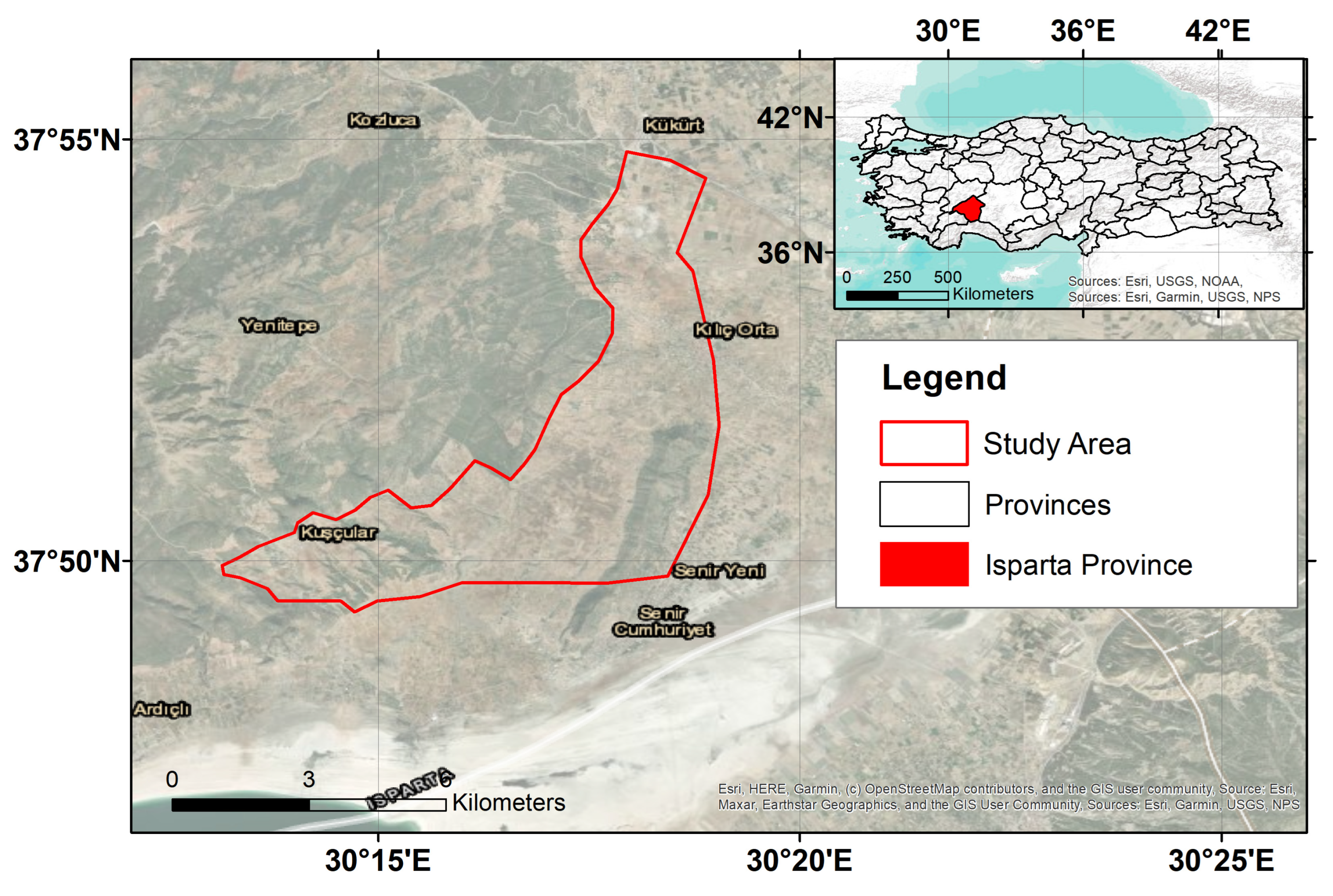
The village of Kuyucak is located north of Lake Burdur (Figure 2) and is situated on fertile agricultural lands. The study area covers a total of 4115 hectares, with a significant portion consisting of lavender cultivated fields. The region lies in a transitional zone between the Mediterranean climate and the continental climate predominant in Central Anatolia. Therefore, both climate characteristics are observed within the boundaries of the province. Due to its proximity to Lake Burdur, the region has a moderate climate. The average annual rainfall is 850 mm, and the average temperature is 12 °C [46].
Lavender production in Isparta province is mainly concentrated in villages such as Kuyucak in the Keçiborlu district, as well as Kuşçular, Aydoğmuş, Çukurören, and Ardıçlı villages. Although lavender cultivation has spread to different provinces since 2015, the village of Kuyucak, affiliated with the Keçiborlu district, where lavender cultivation is most intensively practiced, produces the most lavender honey. With the flowering of lavender fields at the end of June, lavender honey production begins with the placement of beehives along the edges of the fields. During the approximately 35–40 day flowering season, hives are harvested, and lavender honey is obtained after about 10 days of harvest, which lasts until the first week of August. There are eight registered beekeepers in the region where lavender honey production is intensively carried out. Approximately 5 tons of lavender honey are produced annually in the region with around 1000 hives. The 17 honey forests established in Isparta cover a total area of 720 hectares, with the vast majority supported by lavender plants [47].
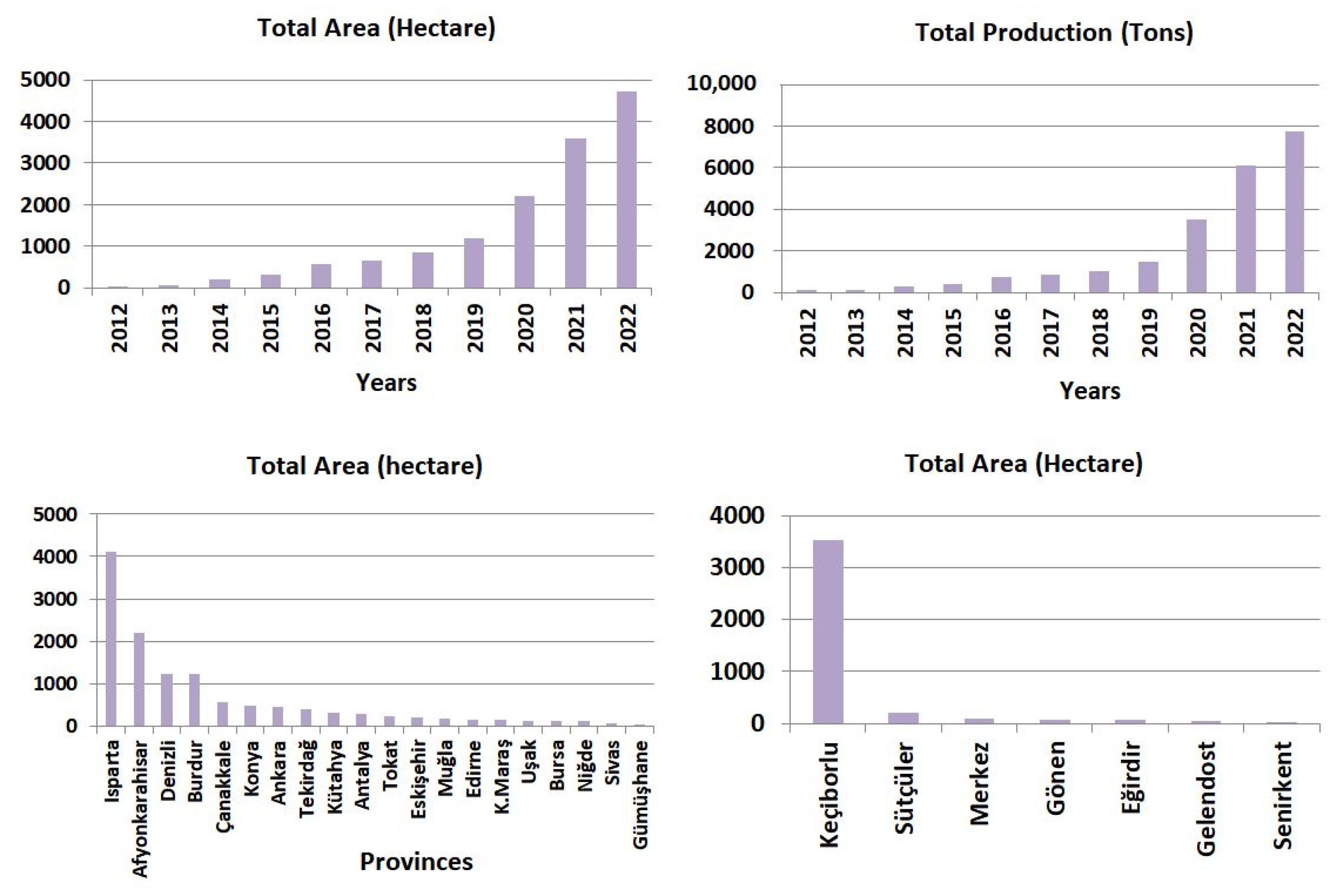
The history of lavender farming in Turkey dates back to the 1970s. Lavender, initially brought from France in the early 1970s, was primarily used as an ornamental plant and began to be cultivated as an industrial product around 1995. Official lavender statistics have been recorded since 2010, with official registered data on lavender production only available after 2015. It can be observed that production areas in the provinces of Afyonkarahisar and Konya were recorded in 2015. In 2015, the lavender production area was 2236 hectares in Isparta province, 900 hectares in Afyonkarahisar, and 82 hectares in Konya. By the year 2020, lavender production was being carried out in 23 provinces [48].
According to data from 2019, Isparta province still has the highest lavender production area (38.4%), followed by Afyonkarahisar (19.5%), Burdur (14.1%), and Çanakkale (9.3%) provinces. Lavender, with its production value increasing every year, creates new lavender honey production areas annually. The district of Keçiborlu in Isparta province has been the leading region in lavender production in Turkey for years. Therefore, in this study, the village of Kuyucak in the Keçiborlu district is addressed due to its significance in lavender production. The statistics for lavender in Turkey are provided in Figure 3.

2.2. Aerial Data

The real true orthophoto images from the year 2020 were used to detect lavenders. The true orthophoto images, captured from approximately 1 km above ground using an aircraft, have a resolution of 30 cm and cover the entirety of Kuyucak district. A total of 4 bands were obtained from the true orthophoto imageries, including 3 bands RGB and 1 band near-infrared. The spectral intervals are 400–580 nm for blue band, 500–650 nm for green band, 590–675 nm for red band and 675–850 nm for near-infrared. The orthophoto images were retrieved in July and the spectral resolutions of the images were 12 bits. The coordinate system of the images is ITRF96 based on GRS80 ellipsoid. Since the orthophoto images are final products, atmospheric and radiometric corrections have been performed by the authorized institution.
Due to the large size of the study area and the intention to apply the developed libraries to different lavender fields, orthophoto images were preferred for both time efficiency and cost-effectiveness. However, orthophotos acquired by authorized institutions for digital map production are typically captured once every five years, with the next scheduled acquisition planned for 2026. Therefore, the 2020 orthophoto dataset was used to demonstrate lavender detectability and to evaluate the performance of the methods. Although higher spatial resolution imagery could be obtained using unmanned aerial vehicles (UAVs), these are significantly more expensive and time-consuming compared to orthophotos. Hence, the use of orthophotos was favored in this study.
For use in classification techniques to detect lavenders, a total of 3750 lavender samples were identified in 4 different sizes and created as a ground truth dataset. These ground truth datasets were used as input for both trained classification methods and deep learning methods.

2.3. Field Data

Since all three methods are machine learning-based, they require training data for classification. To improve accuracy and reduce complexity associated with a high number of classes, four land cover classes were identified in the study area: lavender, bare lands, trees, and green agricultural areas. Given the spectral characteristics of the imagery and the landscape, lavender is typically planted in bare agricultural fields without other vegetation. Therefore, bare land was included as a separate class to maximize inter-class variance. Trees and green agricultural areas, which are spectrally similar to lavender and thus prone to misclassification, were also treated as distinct classes. Additionally, due to the variability in lavender plant sizes and flowering stage, spectral reflectance values differ significantly across the region. To ensure comprehensive representation, training samples were collected from lavender fields of varying sizes and phenological stages.
During the selection of training data, circular regions covering entire lavender plants were used to accurately delineate individual objects. This approach ensures that pixel patterns representing lavender are precisely captured in the training data. As illustrated in Figure 4, the training samples include four different lavender types. To take into consideration the region variability, lavenders samples were collected from different regions across the study area, enabling the models to learn potential variations in lavender characteristics. The training dataset used for both object detection and machine learning classifications are reported in Figure 4.
For training the classification methods, a total of 2612 samples were collected across four different classes. Since the number and distribution of training samples is important for classification performance, attention was given to accurately represent class variance and mean values by covering many pixels. The training datasets included 85,521 pixels (7697 m2) for trees, 45,807 pixels (4123 m2) for green fields, 252,771 pixels (22,750 m2) for bare lands, and 44,298 pixels (3987 m2) for the lavender. A significantly larger number of training samples was collected for the bare lands class due to its high heterogeneity and greater spectral variability compared to other classes. This extensive sampling aimed to improve classification accuracy by highlighting the variability within bare lands. The training sample statistics for both classification and deep learning methods are reported in Table 1.

2.4. Auxiliary Data

2.4.1. Lavender’s Melliferous Potential

The melliferous potential of plants refers to their ability to produce nectar and pollen, which are essential for honey production. If this potential is known, it becomes useful in predicting the amount of nectar a plant can produce, helping to estimate the nectar that can be harvested by bees or other pollinators. This information makes it possible to estimate the amount of honey a hive can produce in a specific area, thus helping to determine suitable areas for beekeeping and optimizing honey production. The melliferous potential (MP) is generally estimated using the following information: (i) the average quantity of nectar secreted by a flower in 24 h, (ii) the sugar concentration of the nectar, (iii) the flower’s lifespan, and (iv) the average number of flowers per unit area or per tree [50]. Consequently, MP is a metric of the nectareous importance of a plant species, varying from species to species and sometimes even between individual plants, as the plant’s age can influence the blooming phase [51,52]. In this paper, MP values for lavender plants were obtained from [53] where MP values is defined as kg·ha−1·y−1 of honey and in the specific case of lavender crop equal to 150 kg·ha−1. This value does not represent the actual quantity of honey obtainable by the beekeeper but rather a theoretical estimate of the melliferous potential of plants under the most favorable conditions.

2.5. Object Detection via Deep Learning

With the rapid advancement of deep learning techniques, Convolutional Neural Networks (CNNs) have become increasingly important for object detection. Compared to traditional handcrafted feature-based methods, deep learning-based object detection methods can teach both low-level and high-level image features. The image features learned with deep learning techniques are more representative than handcrafted features. Object detection has some relationships with object classification, semantic segmentation, and instance segmentation [54]. Deep CNNs are commonly used for object detection. CNN is a type of feedforward neural network that operates on the principle of weight sharing. Convolution is an integration that shows how one function overlaps with another function and is a mixture of the two functions multiplied together [55].
Mask R-CNN is a deep neural network and is an extension of Faster R-CNN, which typically includes an additional branch to predict segmentation masks for each Region of Interest (ROI). Mask R-CNN aims to solve the instance segmentation problem in machine learning and computer vision, distinguishing between objects in an image. It takes an image with one or more objects and returns the image with bounding boxes, classes, and masks. Generally, it consists of two stages. In the first stage, it produces proposals for regions in an input image. In the second stage, it predicts the class of the object along with bounding boxes and generates masks at the pixel level based on the proposals from the first stage. Both stages are dependent on the backbone architecture. Mask R-CNN performs better overall on small, medium, and large objects [56,57].

2.6. Machine Learning Classification

The classification of lavenders was evaluated using ML, SVM, and RF methods to assess their performance in lavender detection. Additionally, object detection based on deep learning was used to independently identify lavenders without classification. The fundamentals of the methods used in the following sections are explained below.

2.6.1. Maximum Likelihood

ML is one of the most used methods for classifying images obtained through remote sensing. In the ML method, a pixel is assigned to a class based on the probability of belonging to that class, which is modeled as a normal distribution in the multispectral feature space [58,59]. The ML method relies on a parametric approach that assumes the selected signature classes follow a normal distribution.
Probability density functions are used to calculate the probability of a pixel belonging to each class for classifying a pixel. During classification, all unclassified pixels are assigned class membership based on the relative probability of the pixel emerging with each class’s probability density function. ML classification is a statistical decision criterion that helps classify overlapping signatures; pixels are assigned to the class with the highest probability [60]. An unknown measurement vector is assigned to the class with the highest probability of belonging. The advantage of ML as a parametric classifier is its incorporation of variance-covariance within class distributions, and for normally distributed data, ML performs better than other known parametric classifications [61].

2.6.2. Support Vector Machine

Support Vector Machines (SVMs) are based on statistical theory and are used in classification and regression problems [62]. The goal of SVM for classification is to determine a hyperplane that best separates two classes [63]. SVMs, also known as support vector machines, are a group of supervised classification methods recently used in remote sensing. The main motivation of SVM is to separate several classes in the training set with a hyperplane that maximizes the margin between them. In other words, SVM allows for maximizing the generalization ability of a model [64].
The classification accuracy produced by SVMs can vary depending on the selection of the kernel function and parameters. Like decision tree classifiers, SVMs are non-parametric classifiers. SVM theory was first proposed by [65] and later extensively discussed by [62]. The success of SVM depends on how well the process is trained. The easiest way to train SVM is to use linearly separable [61]. Generally, SVMs are reported to produce higher accuracy results compared to traditional approaches, but the results depend on the kernel used, parameter selection for the chosen kernel, and the method used to build the SVM [58].

2.6.3. Random Tree Forest

Random Forest is an integrated method that uses clustering and random subspaces to build decision trees [66,67]. It combines multiple decision trees through voting rules. When data is input, the classifier passes the data to each decision tree. Each tree in the forest will have a classification result, and finally, multiple decision trees vote to produce the results [66,68].
A random tree is a tree generated randomly from a set of possible trees, each having K random features at each node. The key point in the term “random” here is that each tree in the forest has an equal chance of being sampled, thereby ensuring a uniform distribution of trees. Additionally, it determines that decision trees have a uniform distribution. In the Random Forest method, the combination of large random trees typically ensures accurate classification [69].

2.7. Accuracy Assessments

The images classified using ML, SVM, and RF methods have undergone accuracy analysis using some accuracy indicators of the classification results include overall accuracy, user and producer accuracy, error of commission, and kappa index (Equations (1)–(5)).
O v e r a l l   a c c u r a c y = C o r r e c t l y   classified   s a m p l e   c o u n t T o t a l   s a m p l e   c o u n t
U s e r   A c c u r a c y = C o r r e c t l y   classified   s a m p l e   c o u n t   T o t a l   classified   s a m p l e   c o u n t   o f   a   c l a s s
P r o d u c e r   A c c u r a c y = C o r r e c t l y   classified   reference   s i t e   c o u n t   T o t a l   c o u n t   o f   reference   s i t e s
K = Pr a P r ( e ) 1 P r ( e )
where Pr(a) represents the actual observed agreement, and Pr(e) represents chance agreement.
The 5 accuracy indicators provided above aim to measure the accuracy of classified images numerically using ground truth data. Overall accuracy is a value calculated as a composite of the accuracy of all classes and is roughly used to determine the accuracy of the classification. Producer and user accuracy are accuracy indicators aimed at showing the accuracy of individual classes. These indicators represent how often real features on the ground are correctly depicted on the classified map or the probability that a certain land cover of an area on the ground is classified as such. User’s accuracy essentially tells us how often the class on the map will actually be present on the ground. Errors of omission are in relation to the classified results. These refer to sites that are classified as reference sites that were left out (or omitted) from the correct class in the classified map. The Kappa Coefficient is generated from a statistical test to evaluate the accuracy of a classification. Kappa essentially evaluates how well the classification performed compared to just randomly assigning values, i.e., did the classification do better than random [70,71,72,73,74,75,76].

2.8. Mapping Melliferous Potential of Lavenders

Once the lavender crop within the AOI was mapped, it became possible to attribute the melliferous potential. It is important to note that the apiary is where honeybee hives are kept, while the beehive is the enclosed structure where bees live and raise their young. The beehive is typically cubic in shape, with dimensions of approximately 50 × 50 × 40 cm. For proper hive placement, certain guidelines should be followed: (i) maintain a 50 cm distance between hives to prevent drift (i.e., hive confusion) during the bees’ return; (ii) align hives in short rows to avoid drift; and (iii) ensure a row spacing of >2 m. Generally, one person can manage about 50 hives per day, making it reasonable to assume a single apiary of that size covers an area of about 100 m2 (10 m × 10 m). Specifically, 10 hives could be arranged in a row 10 m long (50 cm for each hive plus 50 cm of space between hives), with five rows of similar size spaced 10 m apart (50 cm for each hive plus 2 m between rows). To match this granularity, the map of melliferous potential attributed to the lavender plants was rasterized with a pixel size of 10 m. Since the melliferous potential was given in kg·ha−1·y−1, it was necessary to divide the value by 100 to correctly assign it to a 100 m2 pixel. The resulting raster layer is hereafter referred to as MPL(x,y). Finally, after identifying, classifying, and mapping individual lavender plants, it was possible to refine MPL(x,y). Initially, the lavender’s melliferous potential value is estimated assuming the field is fully covered with plants. However, as shown in Table 2, some areas have gaps in coverage. This naturally limits the melliferous potential of each pixel. For example, if only 30% of the field or pixel is covered with lavender, it is necessary to adjust the corresponding melliferous potential, reducing its value according to the actual coverage. Accordingly, the percentage of plant coverage within the lavender field was calculated, and a new map of potential melliferous lavender map was computed (hereafter called MPLP(x,y), taking into account the reduction factor due to the true presence of plants.
MPLP(i) = LMP/100 × CFi
where LMP corresponds to the melliferous potential of lavender (equal to 150), divided by 100 to obtain the melliferous potential value at the pixel level (100 m2) and CFi represents the actual fraction of lavender within i-100 m2 pixel, thus accounting for any gaps or missing crops coverage.

2.9. Optimal Hive Placement to Maximize Lavender Honey Production

The bees’ foraging area can vary considerably depending on nectar availability. Generally, to optimize time, bees tend to forage in areas close to the hive; however, when nectar availability is low, they may travel several kilometers from the hive [20,77,78]. A bee can potentially explore every melliferous flower within an area of approximately 28 km2 (considering a circular home range with a 3 km buffer). To map the total amount of lavender nectar available to a single hive at any given location, a sliding window approach (radius = 3 km, i.e., 300 pixels) was applied to the MPL(x,y). The total local melliferous potential was calculated by summing the melliferous potential values of all lavender pixels within the window. This sum was assigned to the pixel at the window’s center in a new raster layer, referred to as potential bees lavender foraging (PBLF(x,y)). The PBLF is intended to provide a map of the estimated maximum honey that a beehive at a specific location in the study area can harvest, thus allowing the identification of suitable and productive honey areas. It is worth highlighting that distance affects the foraging activity of bees. For the same plant species, nectar produced closer to the hives is collected more quickly and therefore has a greater impact on the amount of honey produced, whereas plants located farther away have a lower impact on the nectar collected. Since the aim is to assess the suitability of a specific melliferous area for hosting beehives, it can be assumed that all plants produce a certain amount of nectar under optimal conditions, and honey production is higher the closer the hives are to the nectar source, as reflected by the sum of honey potential at the pixel level.

3. Results and Discussions

3.1. Machine Learning Classification

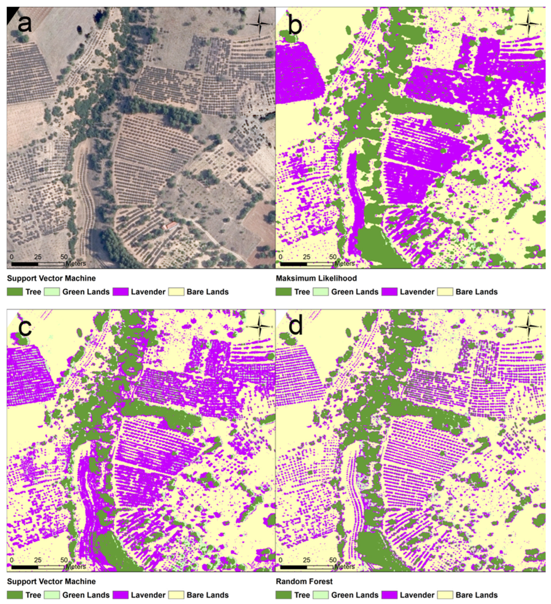
The designated training dataset was utilized with ML, RF, and SVM methods to perform three distinct classifications for the study area. Using these methods, raster imagery was classified into land-use classes of Trees, Green Lands, Lavenders, and Bare Lands to enable clear identification of lavender areas. Visual examination of the classification results revealed that the ML and SVM methods overestimated the size and distribution of lavender clusters, whereas the RF method provided classifications closely matching the actual lavender sizes. Due to the high contrast between Bare Land and Green Land classes compared to other classes, they were classified with high accuracy. However, in all three classification results, shadow areas surrounding trees were misclassified as lavender. To prevent these areas from negatively affecting classification accuracy, they were initially classified and excluded from the imagery using unsupervised classification techniques. Since there are no other black-colored regions in the study area except for shadows, this process effectively isolated shadows as a separate class.
During classification with SVM and RF algorithms, the Radial Basis Function (RBF) kernel was employed in SVM due to the complex structure of lavender plants. For the RF algorithm, a maximum tree depth of 80 and a maximum number of 250 trees were selected. These parameters were determined through extensive experimentation, selecting the values that yielded the best detection performance for lavender.
Given the large extent of the study area, a portion of the classified area is presented in the figure to visually compare the results obtained from ML, SVM, and RF methods. The classification results are given in Figure 5.
To determine and compare the results, the classified images were converted to polygons via raster to polygon tool. Upon examining the classification results, the ML method identified 8.4 km2 as the tree class, whereas the RF and SVM methods identified 3.41 km2 and 3.39 km2, respectively, for the same class. Regarding the lavender class, the ML method identified 1.53 km2, while the RF and SVM methods identified 6.46 km2 and 3.13 km2, respectively. The fact that the ML method classified significantly more trees and fewer lavender areas compared to the other methods suggests that many lavender plants were misclassified as trees. Since the study area predominantly consists of trees and lavender in terms of vegetation, these two classes are the most critical for influencing classification accuracy. While the RF and SVM methods yielded comparable results for the tree class, the RF method identified nearly twice as much lavender area as the SVM method. For the green and bare lands classes, the areas identified by all methods were generally consistent. The numerical values obtained do not provide direct information about classification accuracy; thus, visual examination and accuracy assessments are required to determine which method produces the most accurate classification. The classified area and their % coverages are summarized in Table 2.
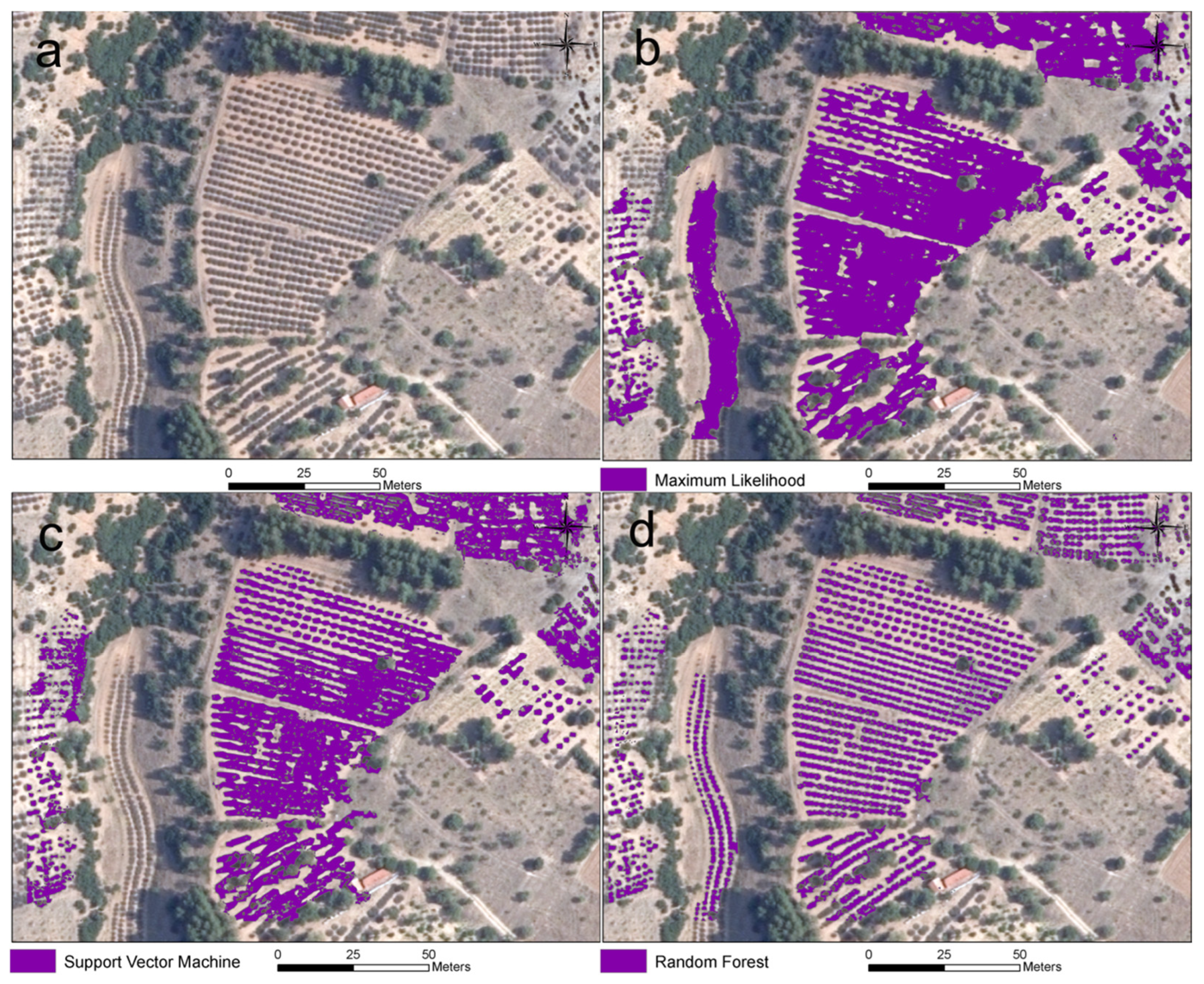
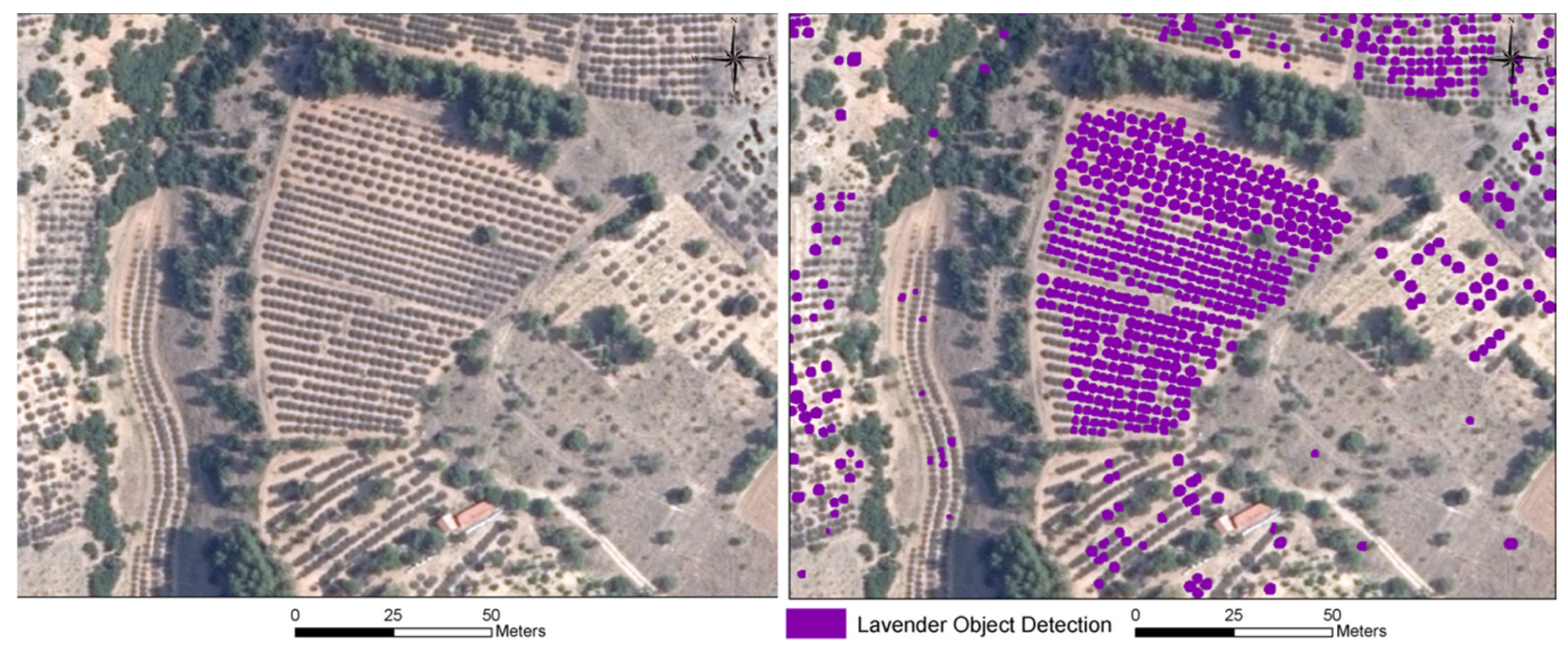
When the classification results are visually examined, it can be observed that classifications created separately according to ML, SVM, RF, and OD methods can detect lavenders. However, in the ML method, lavenders are determined in adjacent areas and tend to cluster in more scattered areas. In the SVM method, the clustering of lavenders is much less compared to the ML method, but lavenders are still determined in clustered areas, close to each other. Due to the importance of spatial values and quantity of lavenders, it has been observed that lavenders identified by ML and SVM methods cover much larger areas than they actually do and are determined in fewer numbers. In the RF method, lavenders are much more distinct and identified as a single object. Especially in combined and separate lavenders, the spatial value is very close to the exact lavender counts, but the number of lavenders is determined less due to the clustering of adjacent lavenders in a single class. Additionally, to assess whether the Random Forest (RF) method results were reliable and not influenced by overfitting, classification outcomes in areas without any sample data and on lavender types not included in the training samples were examined. It was found that lavenders in these regions were accurately detected, with no misclassified lavender areas observed. Therefore, the possibility of overfitting was ruled out. The results in a sample location were given in Figure 6.

3.2. Deep Learning Object Detection

In the Object Detection (OD) method, although lavenders are detected independently, the failure to detect these parts is observed because each of the adjacent lavenders forms a different clustering. Therefore, using any method alone does not fully ensure accuracy in terms of both spatial and numerical aspects due to the growth of lavenders both discretely and adjacently. However, since lavenders cannot be accurately detected numerically in terms of adjacent lavenders from all methods, ensuring spatial accuracy will be a much more accurate approach in detecting lavenders present. Therefore, taking advantage of the RF method’s inability to detect small lavenders and its accurate detection of adjacent lavenders spatially, despite determining larger areas in single lavenders, has been utilized in this study. Similarly, in the OD method, aiming to achieve the closest results to reality both spatially and numerically by using adjacent lavenders from the RF method and single lavenders from the OD method, where single lavenders are correctly identified but adjacent lavenders cannot be fully detected, is aimed. The results obtained with four different methods are shown in Figure 7.
Training of a deep learning method for OD method and detection of lavenders at the end of training was performed using ArcGIS PRO version 2.8.4. A total of 2612 training data were saved as tiles, each with a width of 75 × 75 pixels, using the RCNN Mask method, and metadata files were prepared. The batch size value representing the area around each training data to be learned was set to 4. The backbone model used was a pre-trained image classification network serving as a feature extractor, and specifically, the Resnet-50 model was employed for this study. The model underwent training for a total of 250 epochs, with the training values starting to converge after 150 epochs. During the training phase, the deep learning metrics stabilized after the 160th epoch, leading to early stopping of the process. Subsequently, object detection (OD) was performed on a lavender area with no sample data and exhibiting different shapes. Since lavenders in this region were detected satisfactorily, it was inferred that overfitting did not occur during deep learning.
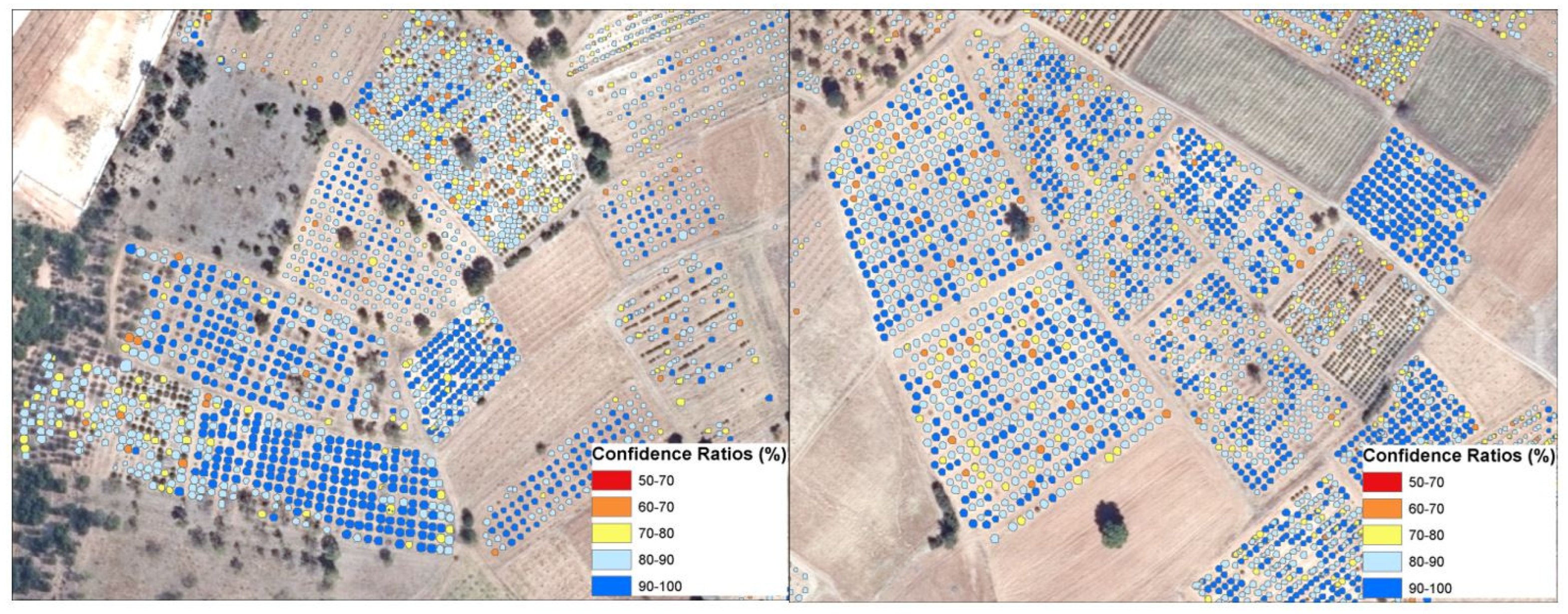
Using the trained model, object detection method was applied with a padding and batch size value of 8, a maximum overlap ratio of 0.1, and a threshold value of 0.5 for detecting lavenders based on confidence intervals. Consequently, lavenders with confidence values above 50% were detected, while those below this confidence threshold were discarded. The learning values of MaskRCNN method obtained for each lavender class and example representations of lavender types are provided in Table 3.
It is observed that the learning values for lavender types 1 and 2 are lower compared to other lavender types. This is because as lavender grows, their branches intertwine, and they are seen more as clusters of lavenders rather than independent lavenders. Consequently, each clustered lavender is perceived as a separate object, resulting in lower learning values. This deficiency has been addressed by comparing it with a dataset obtained from the RF method, where clustered lavender groups are more distinctly identified. Figure 8 illustrates the distribution of confidence values obtained for some regions within the study area.

3.3. Accuracy Assessments

A total of 6000 ground truth points belonging to four different classes, and the results are presented in Table 4. The overall accuracy value indicates the proportion of correctly classified ground truth points to all ground truth points, and it shows that the RF method achieves the most accurate classification with a value of 0.96, while the ML method obtains the lowest accuracy with 0.91. User and producer values have been examined within the scope of accuracy analysis, as they demonstrate the accuracy of individual classes. From the perspective of user accuracy, the lavender class achieves values of 0.90 and 0.95 for ML and SVM methods, respectively, while a value of 0.98 is calculated for the RF method. Thus, the RF method becomes the most accurate classification method for the lavender class. The main reason for this is the wider classification of lavenders in adjacent areas in the ML and SVM methods. Regarding producer accuracy, ML and SVM methods achieve a value of 0.95 for the lavender class, while the RF method determines the lavender class with an accuracy of 0.96. When the accuracy of other classes is examined, the tree class, which is highly likely to be confused with lavenders, achieves a considerably low accuracy value of 0.73 in the ML method. This means that some lavenders are classified as trees, and some trees are classified as lavenders. However, looking at the RF method, it is observed that they are detected with an accuracy of 0.93. In conclusion, considering the kappa index of all classifications, it is seen that the ML method performs classifications with an accuracy of 0.86, SVM with 0.89, and RF method with 0.94 accuracy. Since all accuracy indicators are high in RF analysis, the RF method’s classification result has been used in this study.
To evaluate the accuracy of lavenders detected via object detection (OD), it is necessary to examine which land use class the detected lavenders intersect with. For this purpose, the classified image obtained from the RF method with the highest classification accuracy was compared with the total of 82,353 lavender plants (both individual and clustered) detected via the OD method. Intersection was performed, and the results indicate that lavenders are most confused with the tree class in the classification method’s sensitivity analysis. While 78% of all detected lavenders are entirely lavender, 15% are identified as tree class. This is primarily because the variance of lavenders is very close to the variance of some tree shadows. Lavenders identified as agricultural or green areas make up only 7% of the total data. To remove lavenders identified as tree class from the dataset, since the region has a continuous forest structure and there are no forests among lavender fields, this process can be completed with high sensitivity. All detected lavenders falling within the masked forest boundary of the region were removed. Thus, the accuracy of the OD result was evaluated to be 93%. Objects identified as agricultural or green areas but detected as lavender are mainly due to small shrubs in agricultural areas being misclassified as small lavenders. This issue can be addressed by removing single lavenders from the dataset outside of clusters, as lavenders are typically planted in clusters rather than individually.

3.4. Result Lavender Map

Since the RF method provided the most accurate classification results, the RF results were combined with the OD results to generate the final lavender map. In this way, both clustered and isolated lavenders were obtained based on their sizes and numbers. To combine the results obtained from the RF and OD methods, union and erase overlay analyses have been used. These analyses were employed to delete the areas that were identified in common in both analyses, allowing for the detection of lavenders identified differently in each analysis. Thus, areas identified as adjacent lavenders by the RF method but not present in the OD method could be directly obtained. With the union analysis, the adjacent lavender areas from the RF method are combined with the single lavenders from the OD method, enabling the detection and classification of lavenders in the study area. The resulting product contains lavenders that are very close to the real value spatially but slightly fewer in number in terms of lavender count (Figure 9). In total 104,868 lavenders were detected as a result of the merger process.
The accuracy analysis of the final classification map was conducted using a total of 5469 known lavender points, obtained by combining 2612 lavender points used for training in the Object-Based (OD) method and 2857 lavender points from a set of 6000 ground truth points used for other classification methods. As a result of the analysis, it was determined that 5411 out of the 5469 known lavender points were correctly identified in the final classification map, corresponding to an overall accuracy of 98.9%. The 58 undetected lavender points were generally found to be associated with small lavender plants. While the highest lavender class accuracy achieved using individual classification methods was 98% with the Random Forest (RF) method, this value increased to 98.9% when the results were combined. This indicates that combining the results of the OD and RF methods enabled the identification of a greater number of existing lavender plants.
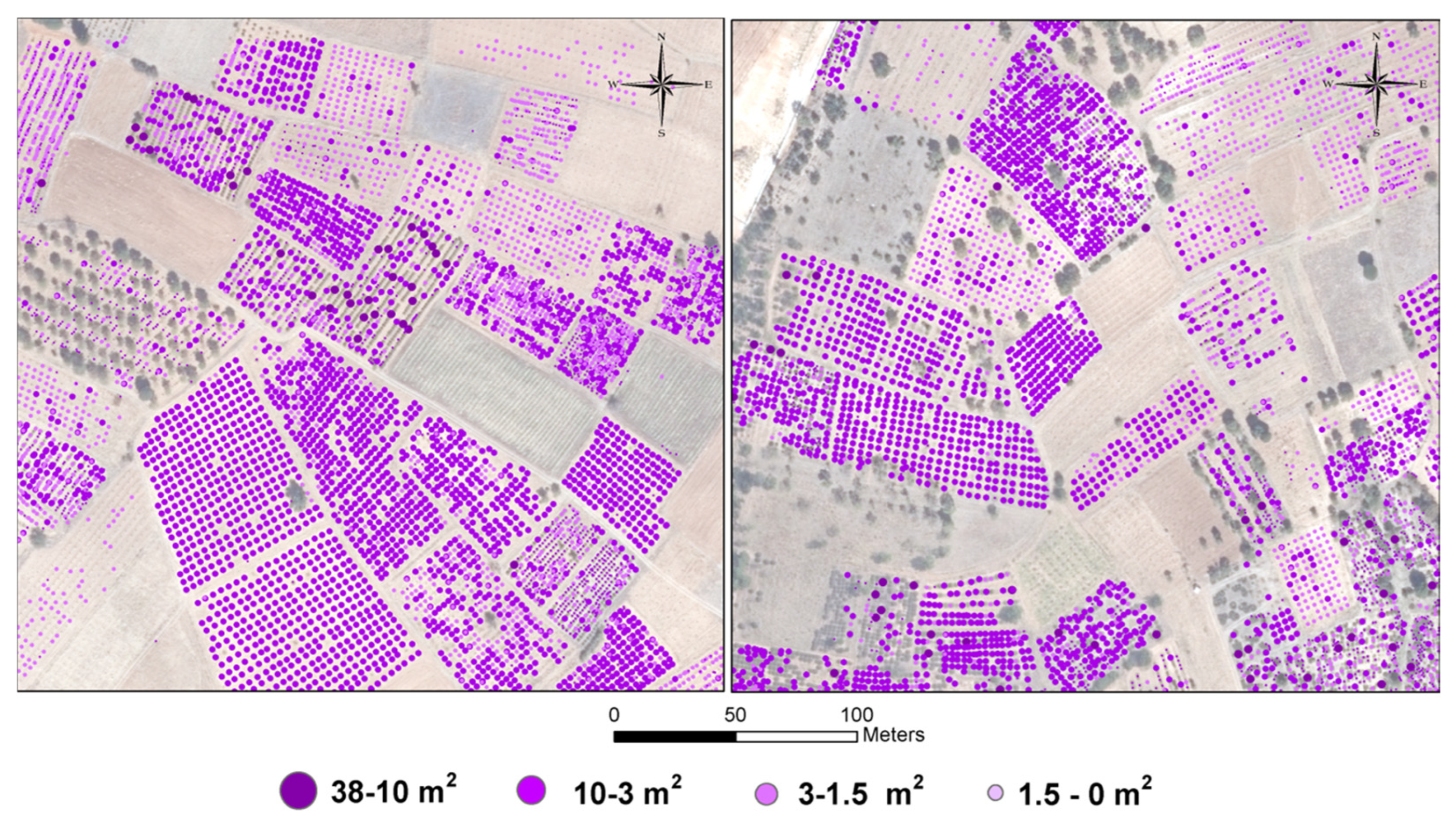
The sizes of lavenders were calculated based on the areas in the classified data. Therefore, both individually and collectively detected lavenders have an area value. Lavenders detected by object detection (OD) methods have been assigned area values directly as a result of the method, so their sizes have been determined based on their area values. Since lavenders were identified as areas directly by both classification and OD methods, centroid analysis was used to represent each lavender as an independent point. Additionally, area values were assigned to the centroids of each lavender, representing each lavender with both point and area values. Lavenders, ranging from the smallest 0.2 m2 to the largest 38 m2 in size, are represented according to their sizes in the classified image as shown in Figure 10.

3.5. Mapping Melliferous Potential of Lavenders

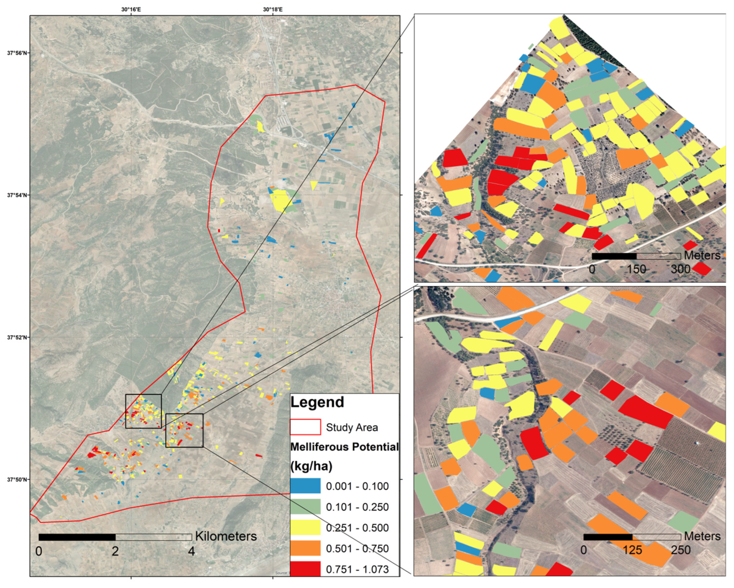
Once the lavender plants within the AOI were mapped, it was possible to attribute the value of the lavender melliferous potential to the identified lavender pixel. MPLP(x,y) is reported in Figure 11.
Lavender (Lavandula spp.) is considered a valuable melliferous plant due to its high nectar production and extended flowering period. However, its honey yield is relatively low compared to other species, such as Robinia pseudoacacia, which can produce up to 500–1000 kg/ha, while lavender typically yields only 100–150 kg/ha [52]. Furthermore, the spatial distribution and density of lavender plants significantly influence nectar availability; sparse plant arrangements can reduce foraging efficiency, thereby lowering honey yields. Considering Figure 12, although the theoretical melliferous potential of lavender is approximately 150 kg/ha, this value decreases considerably when corrected for the high internal variability within fields. Specifically, the potential yield drops to a range of 10–110 kg/ha. This finding underscores the critical role of plant vigor, health, and growth status in determining flower production and, consequently, nectar availability. This reduction occurs independently of adverse climatic conditions, which can further compromise nectar production. This result was expected since, as highlighted in Section 2.4.1, the potential production of the plants occurs only if the plants are in optimal conditions. Consequently, the generated maps are valid only as long as these conditions are met. Given these insights, mapping crop species suitable for melliferous production becomes important to support a beekeeping sector that is increasingly vulnerable to climate variability. Extreme weather events are already known to reduce, or even entirely damage, flowering and nectar production in many plant species [79,80].

3.6. Optimal Hive Placement to Maximize Lavender Honey Production

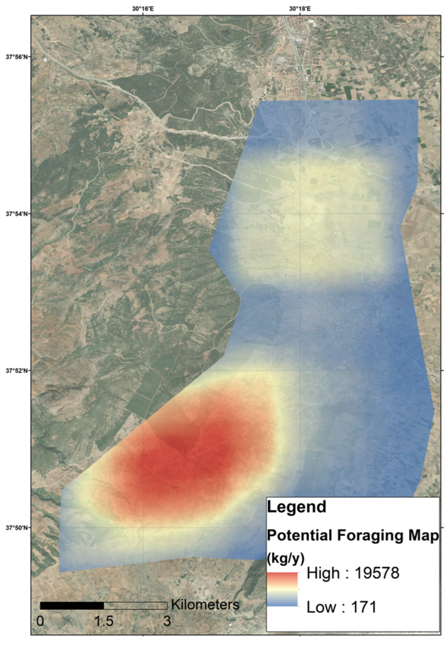
Once the MPLP(x, y) was generated and the fields with a significantly higher melliferous potential were identified, the potential bee foraging map was estimated at the pixel level to assess honey potential production in an apiary located within a specific pixel.
Considering Figure 12, the potential lavender honey yield that bees could collect within a 3 km buffer around an apiary was highlighted. The estimated values range from only a few kilograms to as much as 17,000 kg per year, representing the total nectar-producing potential of lavender crops at the pixel level within the defined buffer zone. The map shows high and low productivity areas. In particular, the southeastern region results to be suitable for lavender honey production, owing to the high concentration of lavender fields. A moderately favorable area is also observed in the northern part of the study area, while the western region shows significantly lower honey potential. Therefore, hive placement in the western zone is not recommended, as the distance from nectar sources may impede colony development.
It is important to note that the estimated honey potential does not directly reflect the actual quantity of honey that beekeepers can harvest. Real-world production is influenced by several additional factors, including environmental conditions and beekeeper management practices, which are not accounted in this analysis. Moreover, the lack of comparable studies in the literature and the absence of field validation with data from local beekeepers make it difficult to assess the accuracy of these estimates.
However, when comparing the findings of this study with existing literature, it becomes evident that few studies specifically address how managing apiary density can enhance honey production, particularly for lavender crops. One notable exception is [22], who explored the use of GIS to reduce competition among bees, potentially caused by local overcrowding. In contrast, the present work considers both foraging zones, distribution of melliferous plants and the specific number of plant available after the classification process, aiming to optimize beekeeping practices within AOI.
Most prior research, however, has focused on identifying favorable environmental conditions—such as vegetation type and water availability—for beekeeping and on generating suitability maps to guide honey production [1,4,81,82]. Nevertheless, no previous work has gone into such detail as to count the specific number of plants and thereby calibrate the potential honey yield.
Other studies have limited their assessments to spatial data and GIS applications for pollinator management and colony loss reduction. For example, [83] combined landscape metrics with crop maps to model bee foraging behavior and colony dynamics, while [84] analyzed relationships between plant species and bee foraging patterns using GIS. More recently, [85] identified priority areas for apiculture development with GIS, proposing maps of potentially productive zones based on local floral resources and plant species composition.
Future research should focus on validating model outputs through field observations and integrating additional variables to improve prediction reliability. Furthermore, it would be interesting to include, in the calculation of pixel-level melliferous potential value, the effect of the distance between the hive and the nectar source, in order to weight the summation proposed in this work and obtain more calibrated results.
In this study, validation against existing honey production data was not possible. Although the region possesses significant potential for lavender honey production, it is also a popular destination for lavender tourism, attracting many domestic and international visitors during the summer months. To prevent any negative impact on tourism, authorities have prohibited beekeepers from settling in the area. Currently, only five beekeepers operate in the region, while many others interested in producing lavender honey wish to establish themselves there. Due to the high demand and the recognized potential, this restriction is planned to be lifted in 2026, allowing beekeepers to settle in the region. Following the settlement of beekeepers in 2026, the production data obtained can be compared with the findings of this study to provide an additional validation of the results.
Despite these limitations, the model provides a valuable preliminary tool for guiding hive placement and apiary management. Beekeepers can use these insights to optimize hive distribution by targeting areas with the highest nectar availability. For example, in zones with low honey potential, reducing hive density or relocating hives to more productive areas may help prevent overpopulation and reduce competition for resources. Such strategic planning can enhance honey production efficiency while also supporting a sustainable balance between managed and wild pollinator populations.

4. Conclusions

In Turkey, beekeepers typically select their production sites based on personal experience, which leads to complexity and prevents a full assessment of regional potential. Furthermore, the lack of comprehensive knowledge about the total potential in study areas, such as the one in this research, hinders institutions and beekeepers from fully utilizing available resources. Therefore, studies like this are crucial for accurately determining potential and identifying optimal locations for beekeeper settlement, enabling sustainable and manageable honey production. Consequently, the potentials of monofloral honey types produced in Turkey—such as lavender, citrus, linden, and sunflower honey—can be determined using these methods. Particularly, the significant increase in citrus and sunflower cultivation in recent years, combined with climate change-induced droughts that reduce production capacity, make it essential for beekeepers to settle in these areas to maintain their colonies and production. In monofloral honey types, where pollen and nectar sources can be quantified as demonstrated in this study, it becomes possible to estimate the approximate honey yield, as well as the maximum number of colonies and beekeepers that can be sustainably established in a region. This approach enables the maximum number of beekeepers to utilize these resources effectively. Moreover, within the framework of climate change, this work contributes by enabling the beekeeping sector and individual beekeepers to constantly monitor vegetation and specific nectar plants in the landscape and surrounding environment (including limiting factors such as water availability), thereby allowing the generation of dynamic maps to identify the most productive areas for hive placement and supporting their annual honey production.
Additionally, due to the pollination role of bees, interdisciplinary studies involving the agriculture and horticulture sectors can be conducted to investigate both beekeeper settlement and the impact of pollination. Especially in fruit orchards such as citrus, apple, peach, plum, apricot, pomegranate, and pear, classification and deep learning techniques applied in this study can help determine suitable production sites for beekeepers and enhance pollination to increase yields for producers. Therefore, conducting such studies across all honey-producing plants and agricultural areas will contribute significantly to the optimal use of national resources and support rural development.

Author Contributions

Conceptualization, F.S. (Fatih Sari) and F.S. (Filippo Sarvia); methodology, F.S. (Fatih Sari) and F.S. (Filippo Sarvia); software, F.S. (Fatih Sari) and F.S. (Filippo Sarvia); validation, F.S. (Fatih Sari); formal analysis, F.S. (Fatih Sari) and F.S. (Filippo Sarvia); investigation, F.S. (Fatih Sari) and F.S. (Filippo Sarvia); resources, F.S. (Fatih Sari) and F.S. (Filippo Sarvia); data curation, F.S. (Fatih Sari); writing—original draft preparation, F.S. (Fatih Sari) and F.S. (Filippo Sarvia); writing—review and editing, F.S. (Fatih Sari) and F.S. (Filippo Sarvia); visualization, F.S. (Fatih Sari) and F.S. (Filippo Sarvia). All authors have read and agreed to the published version of the manuscript.

Funding

This research received no external funding.

Data Availability Statement

The data presented in this study are available on request from the corresponding author.

Conflicts of Interest

The authors declare no conflicts of interest.

References

  1. Maris, N.; Mansor, S.; Shafri, H. Apicultural Site Zonation Using GIS and Multi-Criteria Decision Analysis. J. Trop. Agric. Sci. 2008, 31, 147–162. [Google Scholar]
  2. Oldroyd, P.B.; Nanork, P. Conservation of Asian honey-bees. Apidologie 2009, 40, 296–312. [Google Scholar] [CrossRef]
  3. Estoque, R.C.; Murayama, Y. Suitability Analysis for Beekeeping Sites in La Union, Philippines, Using GIS and Multi-Criteria Evaluation Techniques. Res. J. Appl. Sci. 2010, 5, 242–253. [Google Scholar] [CrossRef]
  4. Estoque, R.C.; Murayama, Y. Suitability Analysis for Beekeeping Sites Integrating GIS & MCE Techniques. In Spatial Analysis and Modeling in Geographical Transformation Process; Springer: Dordrecht, The Netherlands, 2011; ISBN 978-94-007-0670-5. [Google Scholar]
  5. Damián, G.C. GIS-Based Optimal Localisation of Beekeeping in Rural Kenya. Master’s Thesis, Lund University, Lund, Sweden, 2016. [Google Scholar]
  6. Ministry of Agriculture and Forestry. Turkish Beekeeping Statistics. Available online: https://arastirma.tarimorman.gov.tr/tepge/Belgeler/PDF%20%C3%9Cr%C3%BCn%20Raporlar%C4%B1/2022%20%C3%9Cr%C3%BCn%20Raporlar%C4%B1/Ar%C4%B1c%C4%B1l%C4%B1k%20%C3%9Cr%C3%BCn%20Raporu%202022-351%20TEPGE.pdf (accessed on 7 July 2025).
  7. Doğaroğlu, M. Modern Arıcılık Teknikleri Kitabı; Doğa Arıcılık Tic.: Tekirdağ, Turkey, 2004; pp. 64, 65, 87–97. [Google Scholar]
  8. Pehlivan, T. Türkiyede Üretilen Bazı Monofloral Balların Antioksidan ve Antibakteriyel Özelliklerinin Belirlenmesi. Ph.D. Thesis, Mustafa Kemal Üniversitesi, Fen Bilimleri Enstitüsü, Antakya, Turkey, 2015. [Google Scholar]
  9. Gül, A. Türkiye’de Üretilen Bazı Monofolaral Bal Örneklerinin Biyokimyasal Özelliklerinin Belirlenmesi. Türk Tarım Gıda Bilim Ve Teknol. Derg. 2016, 4, 1123–1126. [Google Scholar] [CrossRef]
  10. Adam, K.L. Lavender Production, Products, Markets, and Entertainment Farms; Retrieved November; NCAT: Butte, MT, USA, 2006; Volume 5. [Google Scholar]
  11. Richardson, K. Beekeeping role in enhancing food security and environmental public health. Health Econ. Manag. Rev. 2023, 4, 69–79. [Google Scholar] [CrossRef]
  12. Yusuf, S.F.G.; Cishe, E.; Skenjana, N. Beekeeping and crop farming integration for sustaining beekeeping cooperative societies: A case study in Amathole District, South Africa. GeoJournal 2018, 83, 1035–1051. [Google Scholar] [CrossRef]
  13. Saunders, M.E.; Smith, T.J.; Rader, R. Bee conservation: Key role of managed bees. Science 2018, 360, 389. [Google Scholar] [CrossRef] [PubMed]
  14. Kozuharova, E.; Vereecken, N.J. Lavender production in SE Dobrudja–intensive agriculture impacts pollinators’ density and diversity. Euro-Mediterr. J. Environ. Integr. 2024, 9, 937–943. [Google Scholar] [CrossRef]
  15. Kolayli, S.; Can, Z.; Kara, Y.; Ozkok, A.; Ozmert Ergin, S.; Kemal, M.; Demir Kanbur, E. Physicochemical characteristics, phenolic components, and antioxidant capacities of lavender honey (Lavandula Spp.) from Isparta region of Türkiye. Chem. Biodivers. 2024, 21, e202400718. [Google Scholar] [CrossRef]
  16. Ergin, S.Ö. Antioxidant activity and physicochemical properties of lavender honey enriched with turmeric (Curcuma longa L.). J. Food Meas. Charact. 2025, 19, 1458–1468. [Google Scholar] [CrossRef]
  17. Rhodes, C.J. Pollinator decline–an ecological calamity in the making? Sci. Prog. 2018, 101, 121–160. [Google Scholar] [CrossRef] [PubMed]
  18. Le Conte, Y.; Navajas, M. Climate change: Impact on honey bee populations and diseases. Rev. Sci. Tech. Off. Int. Epizoot. 2008, 27, 499–510. [Google Scholar]
  19. Albacete, S.; Sancho, G.; Azpiazu, C.; Rodrigo, A.; Molowny-Horas, R.; Sgolastra, F.; Bosch, J. Bees exposed to climate change are more sensitive to pesticides. Glob. Change Biol. 2023, 29, 6248–6260. [Google Scholar] [CrossRef] [PubMed]
  20. Greenleaf, S.S.; Williams, N.M.; Winfree, R.; Kremen, C. Bee foraging ranges and their relationship to body size. Oecologia 2007, 153, 589–596. [Google Scholar] [CrossRef]
  21. Van der Steen, J.J.M. The foraging honey bee. BBKA News Br. Bee J. 2015, 2015, 43–46. [Google Scholar]
  22. Awad, A.M.; Owayss, A.A.; Iqbal, J.; Raweh, H.S.A.; Alqarni, A.S. GIS Approach for Determining the Optimum Spatiotemporal Plan for Beekeeping and Honey Production in Hot-Arid Subtropical Ecosystems. J. Econ. Entomol. 2019, 112, 1032–1042. [Google Scholar] [CrossRef] [PubMed]
  23. Vadnais, J.; Perez, L.; Coallier, N. Assessing foraging landscape quality in Quebec’s commercial beekeeping through remote sensing, machine learning, and survival analysis. J. Environ. Manag. 2005, 374, 124157. [Google Scholar] [CrossRef]
  24. Binboğa, Z.M.G.; Demirbaş, N. Türkiye’nin lavanta üretim ve diş ticaretinde ortaya çikan gelişmeler ve mevcut potansiyelin değerlendirilmesi için öneriler. In Proceedings of the Africa 3th International Conference on New Horizons in Sciences, Hurghada, Egypt, 22–25 September 2023. [Google Scholar]
  25. Bah, M.D.; Hafiane, A.; Canals, R. CRowNet: Deep network for crop row detection in UAV images. IEEE Access 2019, 8, 5189–5200. [Google Scholar] [CrossRef]
  26. Velusamy, P.; Rajendran, S.; Mahendran, R.K.; Naseer, S.; Shafiq, M.; Choi, J.G. Unmanned Aerial Vehicles (UAV) in precision agriculture: Applications and challenges. Energies 2021, 15, 217. [Google Scholar] [CrossRef]
  27. Bouguettaya, A.; Zarzour, H.; Kechida, A.; Taberkit, A.M. Deep learning techniques to classify agricultural crops through UAV imagery: A review. Neural Comput. Appl. 2022, 34, 9511–9536. [Google Scholar] [CrossRef]
  28. Shahi, T.B.; Xu, C.Y.; Neupane, A.; Guo, W. Recent advances in crop disease detection using UAV and deep learning techniques. Remote Sens. 2023, 15, 2450. [Google Scholar] [CrossRef]
  29. Richards, J.A. Supervised classification techniques. In Remote Sensing Digital Image Analysis; Springer: Cham, Switzerland, 2022; pp. 263–367. [Google Scholar]
  30. Kotsiantis, S.B.; Zaharakis, I.; Pintelas, P. Supervised machine learning: A review of classification techniques. Emerg. Artif. Intell. Appl. Comput. Eng. 2007, 160, 3–24. [Google Scholar]
  31. Statnikov, A.; Wang, L.; Aliferis, C.F. A comprehensive comparison of random forests and support vector machines for microarray-based cancer classification. BMC Bioinform. 2008, 9, 319. [Google Scholar] [CrossRef] [PubMed]
  32. Santafe, G.; Iñaki, I.; Jose, A.L. Dealing with the evaluation of supervised classification methods. Artif. Intell. Rev. 2015, 44, 467–508. [Google Scholar] [CrossRef]
  33. Prasanna, P.L.; Rao, D.R.; Meghana, Y.; Maithri, K.; Dhinesh, T. Analysis of supervised classification techniques. Int. J. Eng. Technol. 2017, 7, 283–285. [Google Scholar] [CrossRef]
  34. Ahmad, I.; Basheri, M.; Iqbal, M.J.; Rahim, A. Performance comparison of support vector machine, random forest, and extreme learning machine for intrusion detection. IEEE Access 2018, 6, 33789–33795. [Google Scholar] [CrossRef]
  35. Bangira, T.; Alfieri, S.M.; Menenti, M.; Van Niekerk, A. Comparing thresholding with machine learning classifiers for mapping complex water. Remote Sens. 2019, 11, 1351. [Google Scholar] [CrossRef]
  36. Shih, H.C.; Stow, D.A.; Tsai, Y.H. Guidance on and comparison of machine learning classifiers for Landsat-based land cover and land use mapping. Int. J. Remote Sens. 2019, 40, 1248–1274. [Google Scholar] [CrossRef]
  37. Sheykhmousa, M.; Mahdianpari, M.; Ghanbari, H.; Mohammadimanesh, H.; Ghamisi, P.; Homayouni, S. Support Vector Machine Versus Random Forest for Remote Sensing Image Classification: A Meta-Analysis and Systematic Review. IEEE J. Sel. Top. Appl. Earth Obs. Remote Sens. 2020, 13, 6308–6325. [Google Scholar] [CrossRef]
  38. Barghi, B.; Azadeh-Fard, N. Predicting risk of sepsis, comparison between machine learning methods: A case study of a Virginia hospital. Eur. J. Med. Res. 2002, 27, 213. [Google Scholar] [CrossRef] [PubMed] [PubMed Central]
  39. Gislason, P.O.; Benediktsson, J.A.; Sveinsson, J.R. Random forests for land cover classification. Pattern Recognit. Lett. 2006, 27, 294–300. [Google Scholar] [CrossRef]
  40. Cihlar, J.; Latifovic, R.; Beaubien, J. A comparison of clustering strategies for unsupervised classification. Can. J. Remote Sens. 2000, 26, 446–454. [Google Scholar]
  41. Chaovalit, P.; Zhou, L. Movie review mining: A comparison between supervised and unsupervised classification approaches. In Proceedings of the 38th Annual Hawaii International Conference on System Sciences, Big Island, HU, USA, 3–6 January 2005; p. 112c. [Google Scholar]
  42. Enderle, D.I.; Weih, R.C., Jr. Integrating supervised and unsupervised classification methods to develop a more accurate land cover classification. J. Ark. Acad. Sci. 2005, 59, 65–73. [Google Scholar]
  43. Richards, J.A. Clustering and unsupervised classification. In Remote Sensing Digital Image Analysis: An Introduction; Springer: Cham, Switzerland, 2013; pp. 319–341. [Google Scholar]
  44. Olaode, A.; Naghdy, G.; Todd, C. Unsupervised classification of images: A review. Int. J. Image Process. 2014, 8, 325–342. [Google Scholar]
  45. Zou, K.; Chen, Z.; Shi, Y.G.; Ye, J. Object Detection in 20 Years: A Survey. Proc. IEEE 2023, 111, 257–276. [Google Scholar] [CrossRef]
  46. Republic of Türkiye Ministry of Culture and Tourism Official Web Site. Available online: https://isparta.ktb.gov.tr/# (accessed on 16 November 2024).
  47. Isparta Valiliği Official Web Page. Available online: http://isparta.gov.tr/isparta-da-bal-ormanlarinin-sayisi-17ye-ulasti (accessed on 7 July 2025).
  48. Republic of Türkiye Ministry of Industry and Technology. Lavender Farming and Industry Feasibility Report 2020. Available online: https://baka.gov.tr/assets/upload/dosyalar/lavanta-tarimi-ve-endustrisi.pdf (accessed on 16 November 2024).
  49. Turkish Statistical Institute Official Web Site. Lavender Production Statistics. Available online: https://data.tuik.gov.tr/Bulten/Index?p=Bitkisel-Uretim-Istatistikleri-2022-45504 (accessed on 16 November 2024).
  50. Sarvia, F.; De Petris, S.; Borgogno-Mondino, E. Mapping melliferous potential in productive honey areas through spatial tools: Towards a rationalization of beekeeping. Ecol. Inform. 2023, 78, 102362. [Google Scholar] [CrossRef]
  51. Mačukanović-Jocić, M.; Jarić, S. The melliferous potential of apiflora of southwestern Vojvodina (Serbia). Arch. Biol. Sci. 2016, 68, 81–91. [Google Scholar] [CrossRef]
  52. Ricciardelli, D.; Albore, G.; Intoppa, F. Fiori e Api. In La flora Visitata dalle Api e Dagli Altri Apoidei in Europa; Edagricole-Edizioni Agricole della Calderini srl.: Bologna, Italy, 2000. [Google Scholar]
  53. Crane, E.; Walker, P.; Day, R. Directory of Important World Honey Sources; Ulutaş, K., Özkirim, A., Eds.; International Bee Research Association, Minnesota University: Minneapolis, MN, USA, 2018; pp. 30–35. [Google Scholar]
  54. Xiao, Y.; Tian, Z.; Yu, J.; Zhang, Y.; Liu, S.; Du, S.; Lan, X. A review of object detection based on deep learning. Multimed. Tools Appl. 2020, 79, 23729–23791. [Google Scholar] [CrossRef]
  55. Pathak, A.R.; Pandey, M.; Rautaray, S. Application of Deep Learning for Object Detection. Procedia Comput. Sci. 2018, 132, 1706–1717. [Google Scholar] [CrossRef]
  56. Songhui, M.; Mingming, S.; Chufeng, H. Objects detection and location based on mask RCNN and stereo vision. In Proceedings of the 2019 14th IEEE International Conference on Electronic Measurement & Instruments (ICEMI), Changsha, China, 1–3 November 2019. [Google Scholar]
  57. Delight, T.; Karunakaran, V. Deep Learning based Object Detection using Mask RCNN. In Proceedings of the 2021 6th International Conference on Communication and Electronics Systems (ICCES), Coimbatre, India, 8–10 July 2021; pp. 1684–1690. [Google Scholar] [CrossRef]
  58. Huang, C.; Davis, L.S.; Townshed, J.R.G. An assessment of support Vector Machines for Land cover classification. Int. J. Remote Sens. 2002, 23, 725–749. [Google Scholar]
  59. Mondal, A.; Kundu, S.; Chandniha, S.K.; Shukla, R.; Mishra, P.K. Comparison of support vector machine and maximum likelihood classification technique using satellite imagery. Int. J. Remote Sens. GIS 2012, 1, 116–123. [Google Scholar]
  60. Mustapha, M.R.; Lim, H.S.; Jafri, M.M. Comparison of neural network and maximum likelihood approaches in image classification. J. Appl. Sci. 2010, 10, 2847–2854. [Google Scholar] [CrossRef]
  61. Otukei, J.R.; Blaschke, T. Land cover change assessment using decision trees, support vector machines and maximum likelihood classification methods. Int. J. Appl. Earth Obs. Geoinf. 2010, 12, S27–S31. [Google Scholar] [CrossRef]
  62. Vapnik, W.N. An overview of statistical learning theory. IEEE Trans. Neural Netw. 1999, 10, 988–999. [Google Scholar] [CrossRef] [PubMed]
  63. Yang, N.; Li, S.; Liu, J.; Bia, F. Sensitivity of Support Vector Machine Classification to Various Training Features. TELKOMNIKA Indones. J. Electr. Eng. 2014, 12, 286–291. [Google Scholar] [CrossRef]
  64. Cervantes, J.; Garcia-Lamont, F.; Rodríguez-Mazahua, L.; Lopez, A. A comprehensive survey on support vector machine classification: Applications, challenges and trends. Neurocomputing 2020, 408, 189–215. [Google Scholar] [CrossRef]
  65. Vapnik, W.N.; Chervonenkis, A.Y. On the uniform convergence of the relative frequencies of events to their probabilities. Theory Probab. Its Appl. 1971, 17, 264–280. [Google Scholar] [CrossRef]
  66. Breiman, L. Random forests. Mach. Learn. 2001, 45, 5–32. [Google Scholar] [CrossRef]
  67. Khan, Z.; Gul, A.; Perperoglou, A.; Miftahuddin, M.; Mahmoud, O.; Adler, W.; Lausen, B. Ensemble of optimal trees, random forest and random projection ensemble classification. Adv. Data Anal. Classif. 2020, 14, 97–116. [Google Scholar] [CrossRef]
  68. Xu, Y.; Zhao, X.; Chen, Y.; Yang, Z. Research on a Mixed Gas Classification Method Based on Extreme Random Tree. Appl. Sci. 2019, 9, 1728. [Google Scholar] [CrossRef]
  69. Ali, J.; Khan, R.; Ahmad, N.; Maqsood, I. Random forests and decision trees. Int. J. Comput. Sci. Issues IJCSI 2012, 9, 272. [Google Scholar]
  70. Congalton, R.G. A review of assessing the accuracy of classifications of remotely sensed data. Remote Sens. Environ. 1991, 37, 35–46. [Google Scholar] [CrossRef]
  71. Ramsey, E.W.; Jensen, J.R. Remote sensing of mangrove wetlands: Relating canopy spectra to site-specific data. Photogramm. Eng. Remote Sens. 1996, 62, 939. [Google Scholar]
  72. Liu, C.; Fraizer, P.; Kumar, L. Comparative assessment of the measures of thematic classification accuracy. Remote Sens. Environ. 2007, 107, 606–616. [Google Scholar] [CrossRef]
  73. Fung, T.; LeDrew, E. The Determination of Optimal Threshold Levels for Change Detection Using Various Accuracy Indices. Photogramm. Eng. Remote Sens. 1988, 54, 1449–1454. [Google Scholar]
  74. Abd, H.A.A.R.; Alnajjar, H.A. Maximum Likelihood for Land-Use/Land-Cover Mapping and Change Detection Using Landsat Satellite Images: A Case Study South of Johor. Int. J. Comput. Eng. Res. 2013, 3, 26–33. [Google Scholar]
  75. Thoma, M. Analysis and optimization of convolutional neural network architectures. arXiv 2017, arXiv:1707.09725. [Google Scholar] [CrossRef]
  76. Al-Najjar, H.A.H.; Kalantar, B.; Pradhan, B.; Saeidi, V.; Halin, A.A.; Ueda, N.; Mansor, S. Land Cover Classification from fused DSM and UAV Images Using Convolutional Neural Networks. Remote Sens. 2012, 11, 1461. [Google Scholar] [CrossRef]
  77. Osborne, J.L.; Clark, S.J.; Morris, R.J.; Williams, I.H.; Riley, J.R.; Smith, A.D.; Edwards, A. A landscape-scale study of bumble bee foraging range and constancy, using harmonic radar. J. Appl. Ecol. 1999, 36, 519–533. [Google Scholar] [CrossRef]
  78. Gathmann, A.; Tscharntke, T. Foraging ranges of solitary bees. J. Anim. Ecol. 2002, 71, 757–764. [Google Scholar] [CrossRef]
  79. Takkis, K.; Tscheulin, T.; Tsalkatis, P.; Petanidou, T. Climate change reduces nectar secretion in two common Mediterranean plants. AoB Plants 2015, 7, plv111. [Google Scholar] [CrossRef] [PubMed]
  80. Descamps, C.; Quinet, M.; Jacquemart, A.L. Climate change–induced stress reduce quantity and alter composition of nectar and pollen from a bee-pollinated species (Borago officinalis, Boraginaceae). Front. Plant Sci. 2021, 12, 755843. [Google Scholar] [CrossRef] [PubMed]
  81. Zoccali, P.; Malacrinò, A.; Campolo, O.; Laudani, F.; Algeri, G.M.; Giunti, G.; Strano, C.P.; Benelli, G.; Palmeri, V. A novel GIS-based approach to assess beekeeping suitability of Mediterranean lands. Saudi J. Biol. Sci. 2017, 24, 1045–1050. [Google Scholar] [CrossRef] [PubMed]
  82. Abou-Shaara, H.F. Using geographical information system (GIS) and satellite remote sensing for understanding the impacts of land cover on apiculture over time. Int. J. Remote Sens. Appl. 2013, 3, 171–174. [Google Scholar] [CrossRef]
  83. Becher, M.A.; Grimm, V.; Thorbek, P.; Horn, J.; Kennedy, P.J.; Osborne, J.L. BEEHAVE: A systems model of honeybee colony dynamics and foraging to explore multifactorial causes of colony failure. J. Appl. Ecol. 2014, 51, 470–482. [Google Scholar] [CrossRef]
  84. Giannini, T.C.; Chapman, D.S.; Saraiva, A.M.; Alves-dos-Santos, I.; Biesmeijer, J.C. Improving species distribution models using biotic interactions: A case study of parasites, pollinators and plants. Ecography 2013, 36, 649–656. [Google Scholar] [CrossRef]
  85. Marnasidis, S.; Kantartzis, A.; Malesios, C.; Hatjina, F.; Arabatzis, G.; Verikouki, E. Mapping priority areas for apiculture development with the use of geographical information systems. Agriculture 2021, 11, 182. [Google Scholar] [CrossRef]
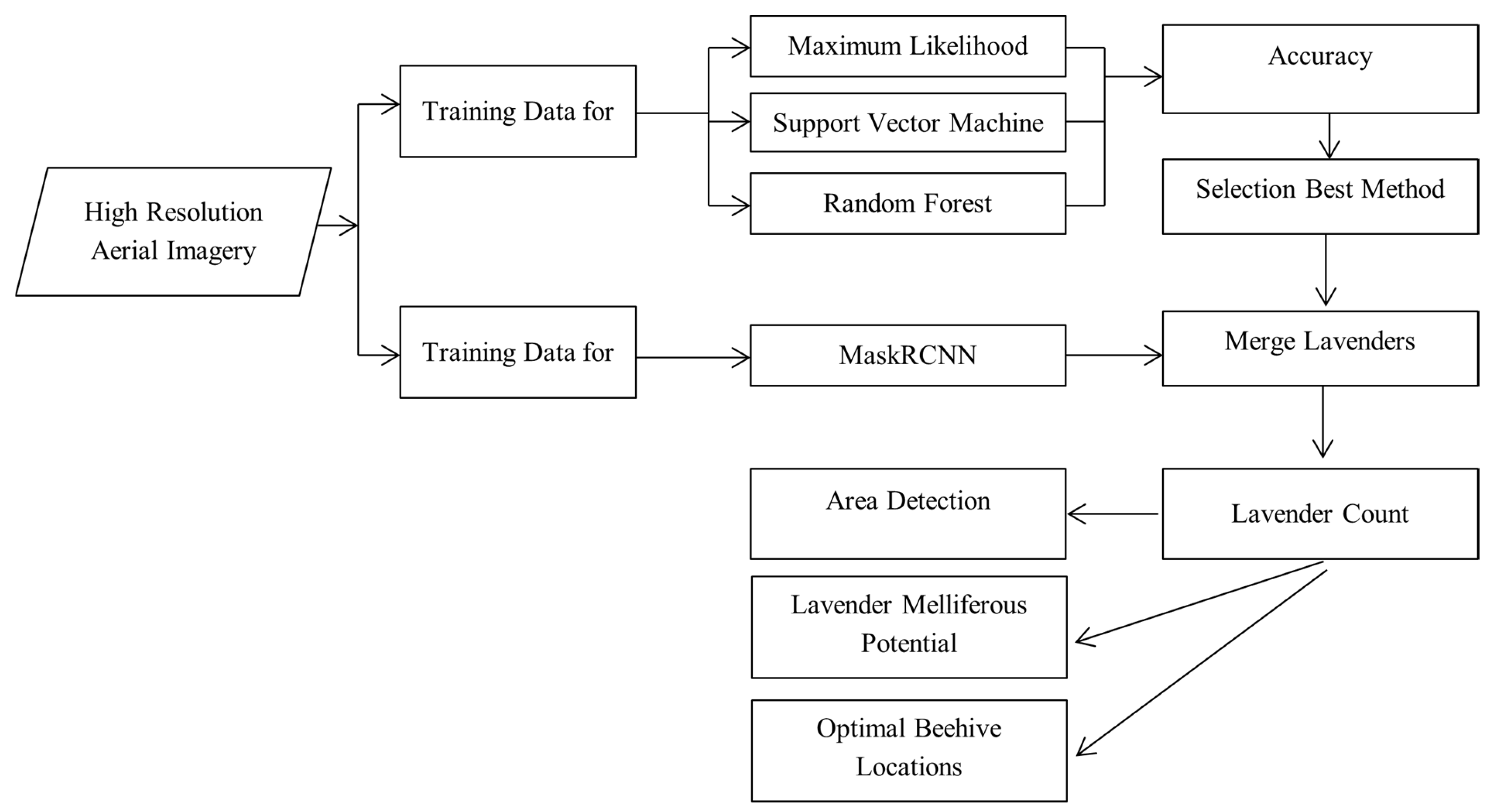
Figure 1. The implementation workflow of the study.
Earth 06 00107 g001
Figure 2. Study area boundaries of Keçiborlu, Kuyucak.
Earth 06 00107 g002
Figure 3. Statistics of Lavender Production in Turkey [49].
Earth 06 00107 g003
Figure 4. Training data for object detection and machine learning.
Earth 06 00107 g004
Figure 5. (a) Original Image, (b) ML, (c) SVM and (d) RF classification results for a sample area.
Earth 06 00107 g005
Figure 6. (a) Classified lavenders via (b) ML, (c) SVM and (d) RF classification methods for a sample area.
Earth 06 00107 g006
Figure 7. Detected lavenders via OD Method for a sample area.
Earth 06 00107 g007
Figure 8. Confidence values of the detected lavenders.
Earth 06 00107 g008
Figure 9. (a) original image, (b) OD results, (c) OD and RF results, (d) Merged lavenders.
Earth 06 00107 g009
Figure 10. Determined area values of lavenders.
Earth 06 00107 g010
Figure 11. Melliferous potential lavender map. Reference system is WGS84/UTM 32 N, EPSG: 32632.
Earth 06 00107 g011
Figure 12. Potential bees lavender foraging map. Reference system is WGS84/UTM 32 N, EPSG: 32632.
Earth 06 00107 g012
Table 1. Training sample counts for classification and deep learning.
Largest Lav.Large Lav.Medium Lav.Small Lav.Total
Deep Learning7157365466152612
TreesGreen FieldsBare LandsLavendersTotal
Classifications5863463018482081
Table 2. Classification results of classes.
MLRFSVM
ClassKm2%Km2%Km2%
Tree8.3927.83.4111.33.3911.2
Green Fields0.531.81.404.71.163.8
Lavender1.535.16.4621.43.1310.4
Bare Lands19.7365.418.9162.622.5074.6
Table 3. Specified parameters for deep learning process and lavender types.
Train Deep LearningObject Detection
Metadata format RCNN MaskPadding8
Batch Size4Threshold0.5
Backbone ModelResnet-50Max Overlap Ratio0.1
Chip Size75Batch Size8
Epochs250
Lavender TypeLearning RateSample Image
Lavender Type 1
(Typically, flowers are in full bloom and have a diameter of more than 1.5 m.)
0.75Earth 06 00107 i001
Lavender Type 2
(The flowers are in bloom and have a diameter of more than 1 m)
0.76Earth 06 00107 i002
Lavender Type 3
(Lavenders with a diameter of up to 0.75 m)
0.83Earth 06 00107 i003
Lavender Type 4
(Lavenders with a diameter of up to 0.50 m)
0.83Earth 06 00107 i004
Table 4. Accuracy assessment statistics of lavender detection.
Maximum LikelihoodSupport Vector MachineRandom Forest
TreeGrassLavenderAgri.TreeGrassLavenderAgri.TreeGrassLavenderAgri.
Error of Omission26.8224.235.022.9711.376.145.009.957.414.133.892.79
Producer Accuracy0.730.760.950.970.890.940.950.900.930.960.960.97
User Accuracy0.890.850.900.930.920.700.930.980.950.830.980.96
Overall Accuracy0.910.930.96
Observed
Agreement (P0)
0.910.930.96
Chance
Agreement (Pe)
0.320.340.35
Kappa0.860.890.94
Disclaimer/Publisher’s Note: The statements, opinions and data contained in all publications are solely those of the individual author(s) and contributor(s) and not of MDPI and/or the editor(s). MDPI and/or the editor(s) disclaim responsibility for any injury to people or property resulting from any ideas, methods, instructions or products referred to in the content.