Geospatial Data and Google Street View Images for Monitoring Kudzu Vines in Small and Dispersed Areas

Abstract

Comprehensive reviews of continuously vegetated areas to determine dispersed locations of invasive species require intensive use of computational resources. Furthermore, effective mechanisms aiding identification of locations of specific invasive species require approaches relying on geospatial indicators and ancillary images. This study develops a two-stage data workflow for the invasive species Kudzu vine (Pueraria montana) often found in small areas along roadsides. The INHABIT database from the United States Geological Survey (USGS) provided geospatial data of Kudzu vines and Google Street View (GSV) a set of images. Stage one built up a set of Kudzu images to be implemented in an object detection technique, You Only Look Once (YOLO v8s), for training, validating, and testing. Stage two defined a dataset of confirmed locations of Kudzu which was followed to retrieve images from GSV and analyzed with YOLO v8s. The effectiveness of the YOLO v8s model was assessed to determine the locations of Kudzu identified from georeferenced GSV images. This data workflow demonstrated that field observations can be virtually conducted by integrating geospatial data and GSV images; however, its potential is confined to the updated periodicity of GSV images or similar services.

1. Introduction

Remote sensing technologies have provided high resolution datasets providing the implementation of machine learning algorithms for exhaustive analyses of invasive species. Monitoring the spread of invasive species aims to develop protocols focused on biodiversity, ecosystem services, and nutrient cycles, among others [1,2]. However, invasive species propagation remains a concern, since dispersion occurs eventually due to anthropogenic activities altering soil, water, and/or endemic vegetation of ecosystems.

Weather, soil, or geomorphology geospatial information retrieved from remote sensing such as satellites, UAVs, and local stations comprise large amounts of data that serve to explain vegetation diversity [3]. These amounts of data require a great demand of computational resources for meaningful maps or statistical analyses aiming to identify invasive species in extensive areas [2]. A suitable option for identification of invasive species is the implementation of a data workflow addressing efficiency and accuracy [4]. Furthermore, the data workflow should consider the use of machine learning tools for overcoming the complexity of the processing tasks.

Some approaches for monitoring and managing invasive species through a geospatial data workflow have followed the species distribution modeling (SDM) or ecological niche models (ENMs) where relationships between known occurrences and environmental characteristics of invasive species can help identify potential regions of expansion. If SDM or ENMs are applied, then target areas with suitability for invasion establishment could be determined, as it was demonstrated in the works of R. Valavi et al. [5] and Callen and Miller [6]. While these commonly used models provide information on where species might be, which can be useful to inform development of watch lists or search activities, managers also require information on where species are currently found. Kudzu (Pueraria montana) is an exemplary case of an invasive species that requires a particular data workflow capable of analyzing extensive geographic areas while ensuring accurate and reliable detection. Kudzu is found across a large range which is still changing, and determining where it is found within that range demands an exhaustive search covering large areas, such as the Eastern United States [4,7,8,9].

To efficiently map a species’ current location across large areas, it is necessary to use data from imagery, such as Kudzu mapping using Sentinel-2 and AVIRIS [10]. Liang et al. [11] identified Kudzu using multispectral images and LiDAR data in one county in Tennessee, US. Their study proposed a two-step classification workflow to reduce computational requirements, which is crucial when analyzing large datasets. Similar studies dealing with multispectral imagery and LiDAR data combined with phenological characteristics [12,13] have been proposed for specific regions. Nonetheless, the opportunity exists for regional examinations of Kudzu due to the range of Kudzu in the conterminous US. Informing invasive plant management decisions requires a specific workflow that integrates automation and human intervention, ensuring broad spatial coverage while maintaining high-resolution analysis at the local scale.

Given these challenges, Google Street View (GSV) offers an alternative [14] that is scalable, cost-effective, and capable of providing high-resolution, temporally updated imagery along road networks worldwide [15]. GSV has been successfully used for plant species identification [16], including invasive alien plants [17], and holds potential for large-scale ecological studies [18]. Its continuously updated image library also allows for temporal analysis of changes in roadside vegetation. Thus, GSV imagery can verify GPS locations and be aligned to ecological models to maximize virtual monitoring supervision of Kudzu.

To achieve the goal of widespread application at a high precision and at the local level, we propose an efficient and accurate data workflow that utilizes georeferenced observations where Kudzu has been observed as the area of interest (AOI). Given that Kudzu distribution is closely associated with human activities and frequently encroaches upon areas near roads and buildings [19], we used the set of AOI for conducting a virtual roadside field campaign that retrieved high resolution images through the GSV application program interface (API), as it has been shown to be advantageous for roadside monitoring [14]. Then, identification of Kudzu in the GSV images was accomplished by means of a trained YOLOv8s object detection model based on convolutional neural networks (CNNs).

This work addresses the problem of automating invasive species monitoring by using publicly available, street-level imagery and machine learning. Its contributions are threefold. First, we conduct a retrieval of images to build a set of Kudzu images for training, validating, and testing an object detection model, particularly YOLOv8s. Second, we implement the use of geospatial data of historical observations aggregated by INHABIT [20] to determine small and dispersed AOIs where Kudzu can be found. Finally, we assess the performance of the workflow at identifying Kudzu from GSV images, to then determine the potential of scalability and implementation for future invasive species monitoring workflows.

1.1. CNNs Applied to Identification of Invasive Species

CNNs are a useful tool for identification of invasive plant species as image analyses requires deep learning [21]. CNN models reduce time-consuming and expensive work from experts in locating a target species so that management actions can be taken [22]. Convolution, Rectified Linear Unit (ReLU), pooling, striding, padding, and fully connected layers organized in specific patterns make the CNN architecture capable of learning and extracting features and kernels from complex pixel arrays [23]. Also, CNN models enable parameter sharing of a kernel applied across different parts of the image. Consequently, the CNN model reduces the total number of parameters in the network compared to traditional CNN architectures, leading to faster training and more efficient computation [24]. These benefits from CNNs aid automatic detection of significant features from images without the need of human supervision [25]. CNN models count on versatility and feasibility for invasive species identification, making them robust tools for image analysis [21,26,27], but challenges remain in determining the appropriate CNN architecture and ensuring a large enough image dataset for training, testing, and validation.

If a pre-trained CNN model is employed for transfer learning, it can facilitate the expansion of the image dataset by enabling efficient annotation or selection of additional relevant images. This approach may enhance model performance by using knowledge from existing models to improve feature extraction and classification accuracy, even when the original dataset is relatively small [22], relying on verified labeled images [28]. In this way, the training and testing phases of the CNN model will have better performance at identifying invasive species. However, an invasive species’ phenology and the species’ relationship with abiotic conditions, including soil and climate, will define its characteristics [29,30], which can be accounted for using a larger number of images from a range of those conditions. The challenge goes further, given that images may not be uniform with respect to aspects such as lighting, pose, distance of image key elements, background, and surrounding objects [23], which should be considered in the image dataset for adequate training and testing phases of a CNN model. Nonetheless, several of these issues are overcome if high-resolution images are used [29].

Researchers and practitioners implementing CNN architectures for identification of invasive species have relied on images from satellites [10,28,30,31], UAVs [27,32,33,34], LiDAR [11,35], or GSV [18]. In addition, others have relied on complementary resources to successfully identify a particular invasive species, for SDM [36], ENMs [37], or databases [4]. Our study found that an effective data workflow for Kudzu identification should rely on two stages in order to cover the conterminous United States. The first stage focuses on generating a dataset of Kudzu images for training CNNs which, in turn, are applied to identify Kudzu in high resolution images retrieved from GSV. The second stage retrieves locations of Kudzu from a database censing historical field observations, such as the one developed by Young et al. [4].

Various CNN approaches are suggested for object detection tasks. Some CNN architectures include OverFeat [38], Region Proposals [39], You Only Look Once (YOLO) [40], and Single Shot MultiBox Detector (SSD) [41], among others. Other object detection methods are non-neural approaches such as the Histogram of oriented gradients (HOG) features [42] or the Scale-invariant feature transform (SIFT) [43]. However, most plant detection studies utilize YOLO models, including versions like YOLOv2 [44], YOLOv4 [45], and YOLOv5 [46,47]. Given its balance of speed and accuracy, YOLOv8s was selected as the primary model for our workflow, as discussed in the following section.

1.2. Object Detection Using YOLO (You Only Look Once) and YOLOv8

This study used YOLOv8, introduced in 2023, which builds upon previous YOLO versions [48] with further enhancements such as the adoption of anchor-free detection, decoupled head architecture, and CSP layers [49]. The You Only Look Once (YOLO) algorithm is a widely used object detection method renowned for its speed and accuracy. It frames object detection as a single regression problem, predicting bounding boxes and class probabilities directly from full images in a single evaluation [40]. This approach differs from traditional methods, which apply classifiers to multiple parts of an image, making YOLO significantly faster [50,51].

In this study, we prioritized a model that balances speed, accuracy, and low computational resource requirements, which are essential for invasive species monitoring, where thousands of locations must be quickly analyzed to mitigate ecological disturbances. Several comparative studies [51,52,53,54] have shown that while Faster R-CNN achieves high detection accuracy, it does so at the cost of significantly higher inference times and memory usage due to its two-stage architecture, making it less suitable for real-time applications or deployment on low-resource devices. On the other hand, SSD offers a compromise between speed and accuracy but consistently underperforms in precision compared to YOLO variants, especially in complex or high-resolution imagery. YOLO models, particularly YOLOv3 and later versions, have demonstrated superior performance in real-time object detection tasks, with competitive accuracy and significantly faster processing speeds—up to eight times faster than Faster R-CNN in some cases. Given these factors, YOLO was chosen since it is particularly well-suited for our application involving the rapid and accurate identification of Kudzu from large-scale roadside imagery datasets.

Since its initial development, YOLO has undergone multiple variations, each introducing architectural improvements to enhance performance. YOLOv8, released in January 2023 by Ultralytics [55], introduces significant advancements over previous versions [48]. One key innovation is its anchor-free detection mechanism, simplifying predictions by focusing on object centers instead of predefined anchor boxes. This modification reduces computational overhead and improves detection adaptability [55]. Additionally, YOLOv8 incorporates advanced data augmentation techniques to enhance model robustness across diverse datasets [49].

The YOLOv8 series includes five model variants—YOLOv8n, YOLOv8s, YOLOv8m, YOLOv8l, and YOLOv8x—each offering a different balance between speed, accuracy, and computational complexity [55,56]. Additionally, YOLOv8 models are pre-trained on the COCO dataset, which contains 91 object categories [57]. In particular, the YOLOv8s model features a lightweight network structure, making it ideal for embedded devices and real-time applications while maintaining strong detection performance [58].

Applications of YOLO extend across various domains [59]. In agriculture, they are used for plant pests and disease identification [60], weed detection and quantification [61], and crop detection [62]. Within biodiversity conservation, YOLO facilitates monitoring animal behavior [63,64], identifying trees in urban environments [45,46], and detecting species in different ecosystems. These applications provide valuable insights into ecosystem health, supporting biodiversity conservation and invasive species management efforts.

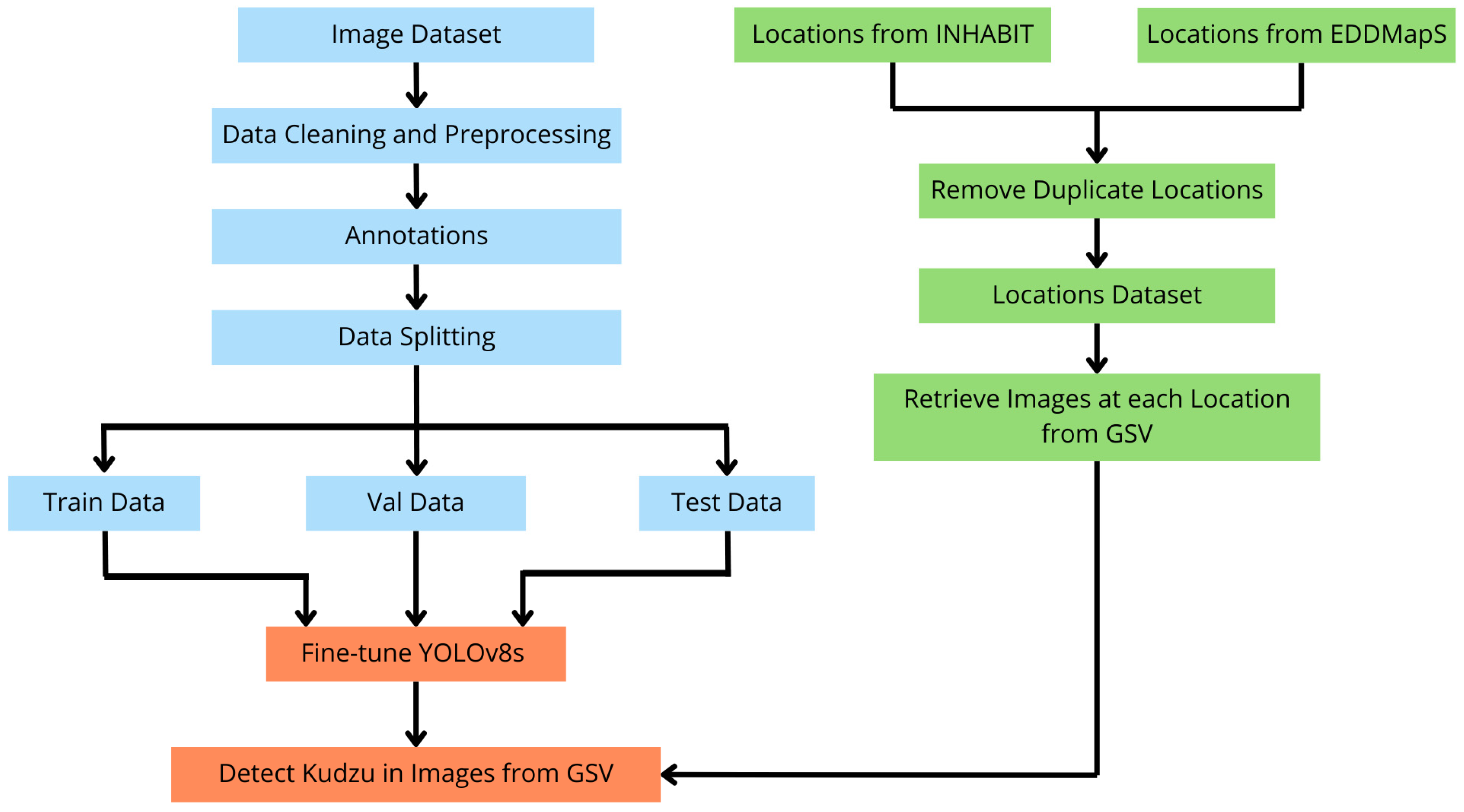
2. Materials and Methods

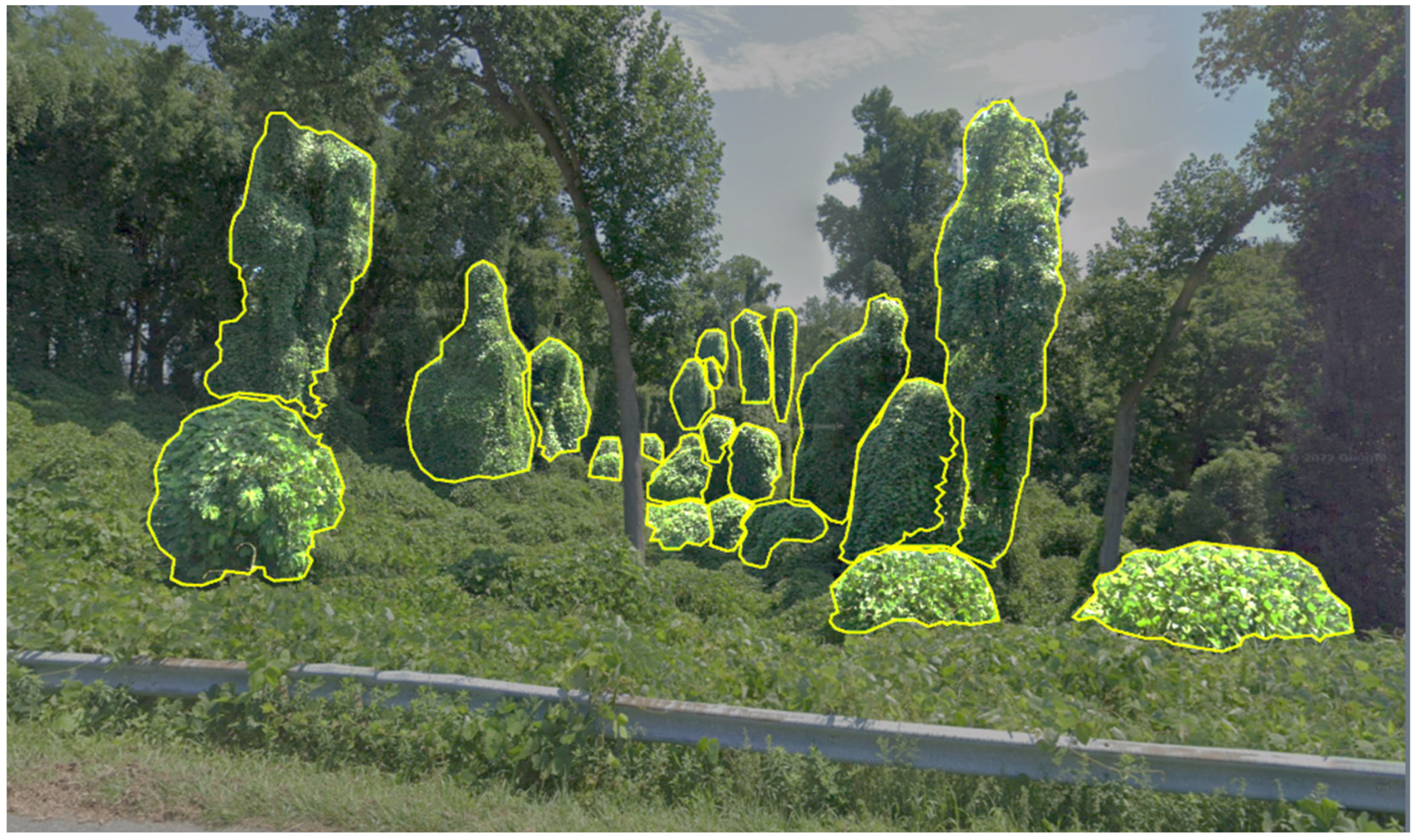
2.1. Definitions for Training, Validation, and Testing Kudzu Images

A training dataset for object detection consisted of images annotated with bounding boxes highlighting Kudzu plants. The collection process involved manually searching for locations containing Kudzu on Google Street View, ensuring a diverse set of visuals that accurately represent multiple camera angles and lighting. Then these images were manually labeled using Roboflow, an annotation tool with AI-assisted annotation to augment human labeling [65]. Figure 1 shows one of the images annotated with Roboflow.

To ensure uniform input dimensions for model training, all annotated images were verified to be 512 × 512 pixels using a center cropping method. Any images that lacked annotations were excluded from the dataset to retain only relevant data. Please note that dead Kudzu vegetation was a challenging factor since its visual properties such as color, texture, and shape change drastically. To augment the number of images, three variations of each training image were generated to enhance model robustness. These variations included random cropping with a zoom range from 0% to 15%, adjusting the hue between −20° and +20°, and changing brightness by ±15%, adding variety and simulating different real-world conditions.

The dataset for object detection comprised 252 images before augmentations. Augmentation increased the dataset to 540 images. Of these 540 images, 432 images were allocated using random sampling for training, while the remaining 20% were reserved for validation and testing, including 10% for each set. Several studies employing YOLO architectures have utilized varying dataset sizes, ranging from approximately 900 to 4500 images [44,45,46]. In contrast, this study prioritized a more restrictive dataset size, a practice that is effective in other computer vision tasks, such as image classification. Shahinfar et al. [66] suggest that datasets with approximately 150 to 500 images per class are sufficient to achieve reasonable classification accuracy. This approach aligns with previous CNN-based studies that utilized a similar number of training images [67,68]. In addition, the number of images for training, validation, and testing is often allocated with 70–80% of data for training and 20–30% for validation and testing, such as in a previous work by Gholamy et al. [69]. A similar study of deep learning (DL), by S. Ahmed et al. [61], also utilized 80% for training and 20% for validation and testing.

2.2. Geospatial Data

A dataset related to invasive species from the Fort Collins Science Center of the United States Geological Survey was used for this research work. In particular, we focused on aggregated occurrence data for Kudzu, used to develop habitat suitability models for the Invasive Species Habitat tool (INHABIT)—a web-based decision support tool of the United States Geological Service (USGS) [20]. The study area encompasses the conterminous United States, focusing primarily on the eastern and southeastern regions where Kudzu (Pueraria montana) is most prevalent. This area is characterized by a humid subtropical climate [70], extensive road networks, and a history of Kudzu invasion, particularly in states such as Georgia, Tennessee, Mississippi, and Alabama. The selection of this area was guided by the availability of comprehensive georeferenced Kudzu occurrence data from the INHABIT tool and the suitability of GSV coverage along major and minor roads. These factors ensure that the workflow is tested in regions with both high ecological relevance and sufficient imagery for model evaluation. The website provides information about GPS-confirmed locations based on historical observations. The GPS-confirmed locations from INHABIT were cross-referenced with those from the Kudzu Early Detection and Distribution Mapping System created by the Center for Invasive Species and Ecosystem Health at the University of Georgia [71]. Duplicate entries were removed, and the combined dataset comprised a total of 28,094 potential Kudzu locations.

Google Street View (GSV) Images

A set of GPS locations where Kudzu was found were used to retrieve images using GSV. This set of images had a resolution of 512 × 512 pixels and could capture roads out to 50 m from road edges, since Kudzu is often observed in locations along roadsides [29]. As a consequence, GSV images had variable pan, tilt, and zoom. Nonetheless, GSV images from roads captured features and characteristics of Kudzu which were needed for successful identification through object detection. In order to capture different angles, the GSV API was configured to save images covering the four cardinal directions (north, south, east, and west) at each GPS location, incrementing by four the number of downloaded images.

2.3. YOLOv8 for Kudzu Detection

The YOLOv8 model by Jocher et al. [55] from the Ultralytics library uses an anchor-free model with a decoupled head to independently process objectness, classification, and regression tasks. This design enhances detection performance by allowing each branch to specialize in its respective task. In the output layer, a sigmoid activation function is applied to the objectness score, indicating the likelihood of a bounding box containing an object, while the softmax function is used to calculate the probability distribution over different classes [48].

A custom dataset comprising annotated images of Kudzu plants was utilized to fine-tune a YOLOv8 small model (yolov8s.pt) using transfer learning. This approach facilitates the adaptation of the model to the Kudzu detection task while reducing the need for data [72]. Given its balance between speed and accuracy, YOLOv8s was selected for its efficiency in object detection, which addresses one of the requirements of this Kudzu identification project.

The YOLOv8s model was trained for 100 epochs using a batch size of 16 images. Training was conducted using the AdamW optimizer with an automatically determined learning rate (lr = 0.002) and a momentum of 0.9. The training process of the YOLOv8s model involved three loss functions: box loss, classification loss, and distribution focal loss (DFL). Box loss measures the accuracy of predicted bounding box locations, used to ensure precise localization of Kudzu plants in images. It was based on Complete Intersection over Union (CIoU) loss, which improves upon traditional IoU-based losses by addressing scale and aspect ratio discrepancies [56,73]. Classification loss was employed to ensure that detected objects were correctly identified. This was implemented using Binary Cross-Entropy (BCE) loss with logits, a stable loss function that integrates a sigmoid layer to enhance numerical performance [74]. Finally, DFL was utilized to refine bounding box predictions by better modeling spatial information and improving localization precision, particularly for challenging object instances [75], like Kudzu. These loss functions were assigned weights of 7.5, 0.5, and 1.5, respectively, optimizing the balance between localization accuracy and classification performance. Non-maximum suppression (NMS) was applied to filter overlapping predictions, ensuring that only the most confident detections were retained. The IoU threshold for object matching was set at 0.7, balancing precision and recall to improve performance. Iterative weight adjustments allowed the model to minimize detection errors and enhance its predictive capabilities.

Once the model was trained, it was integrated into the workflow to identify Kudzu in GSV images. The detection output comprised bounding boxes around detected Kudzu plants. Each detection was assigned a confidence score, representing the probability that the identified object was Kudzu. In summary, Figure 2 shows the full data workflow, from the training dataset to the model fine-tuning and the retrieval of GSV images.

2.4. Metrics of Evaluation of YOLOv8s Algorithm

The YOLOv8s model was validated to assess its generalization performance. The validation process involved running the trained model on unseen data from the same dataset used during training. The metrics included precision, recall, and mean average precision (mAP), which are widely recognized in object detection tasks [76]. This step ensured that our model could reliably identify “Kudzu” in diverse scenarios without overfitting to the training data.

The concept precision, also known as the positive predictive value, is the fraction of relevant instances among the retrieved instances. Also precision is important when the cost of false positives is high, as it indicates how reliable positive predictions are [77,78]. Mathematically, precision is expressed as follows [79]:

$$precision={\displaystyle \frac{TP}{TP+FP}}$$

(1)

where:

$TP$ = True positives (correctly identified Kudzu instances);

$FP$ = False positives (incorrectly identified Kudzu instances).

The concept recall measures the proportion of actual positives that are correctly identified by the model. It is calculated as the ratio of true positives to the sum of true positives and false negatives (missed actual positives) [78]. Mathematically, it is defined as follows [79]:

$$recall={\displaystyle \frac{TP}{TP+FN}}$$

(2)

where:

$FN$ = False negatives (missed Kudzu instances).

Studies on object detection highlight the mAP as an effective metric [80], as it provides insight into both classification accuracy and localization precision [61]. mAP evaluates the precision–recall tradeoff across different confidence thresholds. It is derived by first computing the average precision (AP) for each class, which represents the area under the precision–recall curve [81]:

$$AP={\int }_0^{1}precision\left(recall\right)d\left(recall\right)$$

(3)

The mAP is then calculated by averaging the AP values across all classes [76]:

$$mAP={\displaystyle \frac{1}{N}}{\sum }_{i=1}^N{AP}_i$$

(4)

where:

$N$ = Total number of classes.

One of the most frequently used thresholds is mAP@50, which evaluates mAP at a fixed IoU threshold of 0.5. This means a predicted bounding box must overlap by at least 50% with the ground-truth box to be classified as a correct detection. Due to its more tolerant criteria, mAP@50 generally yields higher values and serves as a widely adopted benchmark in object detection research. Another widely used evaluation metric is mAP@50–95, also known as mAP@COCO, which averages mAP scores across multiple IoU thresholds, ranging from 0.5 to 0.95 in increments of 0.05. This approach results in a stricter evaluation, as higher IoU thresholds demand more precise localization. Consequently, mAP@50–95 is considered a more rigorous metric, reflecting the model’s ability to accurately delineate object boundaries across various levels of overlap. While mAP@50 provides a general measure of detection accuracy, mAP@50–95 offers a more rigorous assessment. Together, these metrics provide a well-rounded assessment of the YOLOv8s model’s effectiveness in detecting Kudzu across various conditions.

2.5. Code Implementation

This project implemented a deep learning pipeline to detect Kudzu in GSV images. The environment set up included PyTorch (version 2.4.1 + cu118), OpenCV (version 4.10.0.84), Matplotlib (version 3.7.5), TorchVision (version 0.19.1 + cu118), Ultralytics (version 8.3.53 + cu118), Roboflow (version 1.1.50), and NumPy (version 1.24.4) for model development and image processing. Additionally, the standard Python 3.9 libraries os, time, math, shutil, json, subprocess, and imghdr were used to manage file operations and handle timing functionalities. For image visualization and evaluation, we used Pillow (version 10.4.0) and Scikit-learn (version 1.3.2). Further information is available at https://github.com/RojanoLab/KudzuDetection (accessed on 9 March 2025) and in Appendix A. The hardware used for YOLOv8s model training, validation, and testing as well as identification of Kudzu from GSV images was a Dell Precision 7920 workstation equipped with 1 GPU (NVIDIA RTX A6000, NVIDIA, Santa Clara, CA, USA); 52-core CPUs (Intel^® Xeon^® Platinum 8270; 2.70 GHz, Intel, Santa Clara, CA, USA), and 187 gigabytes of RAM.

3. Results

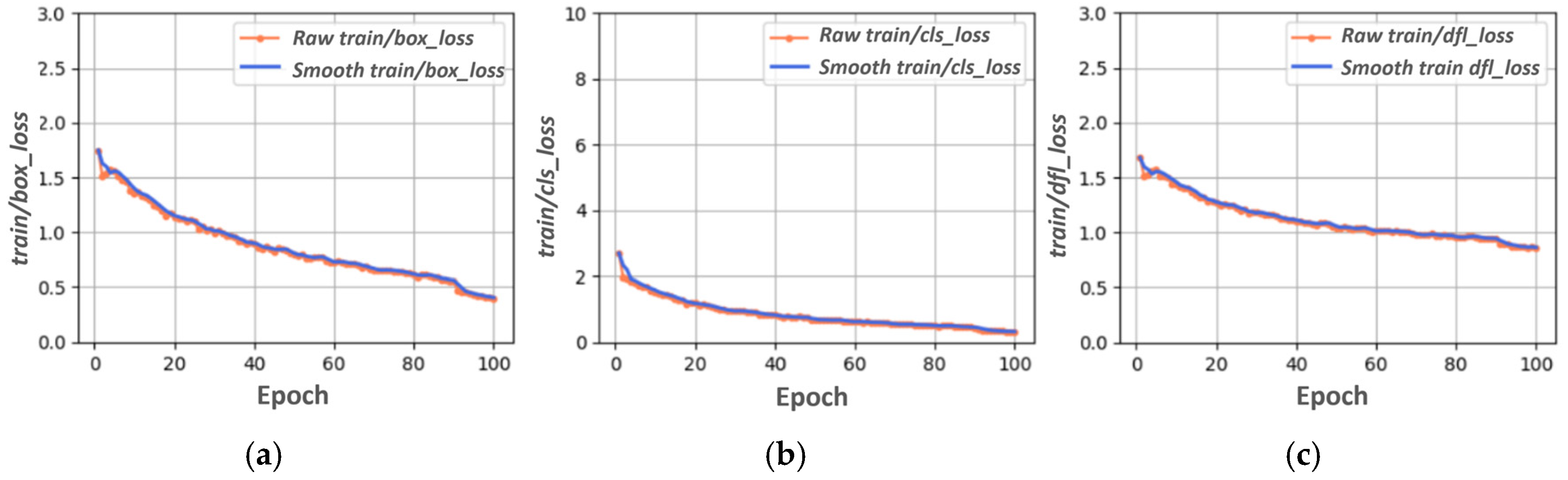
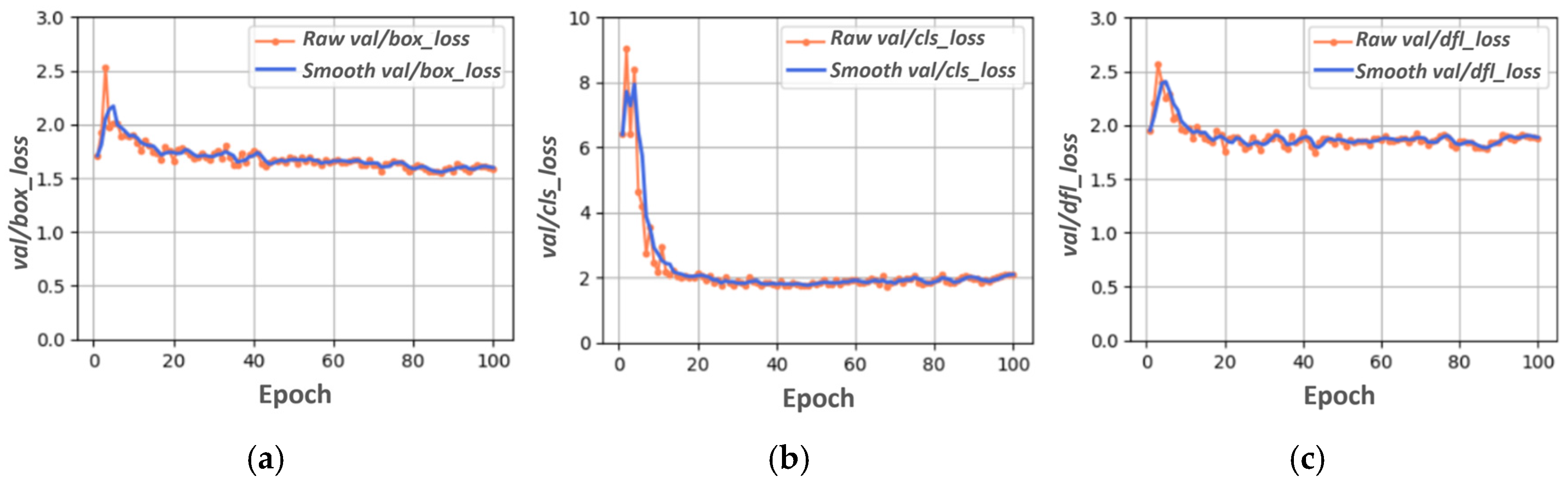
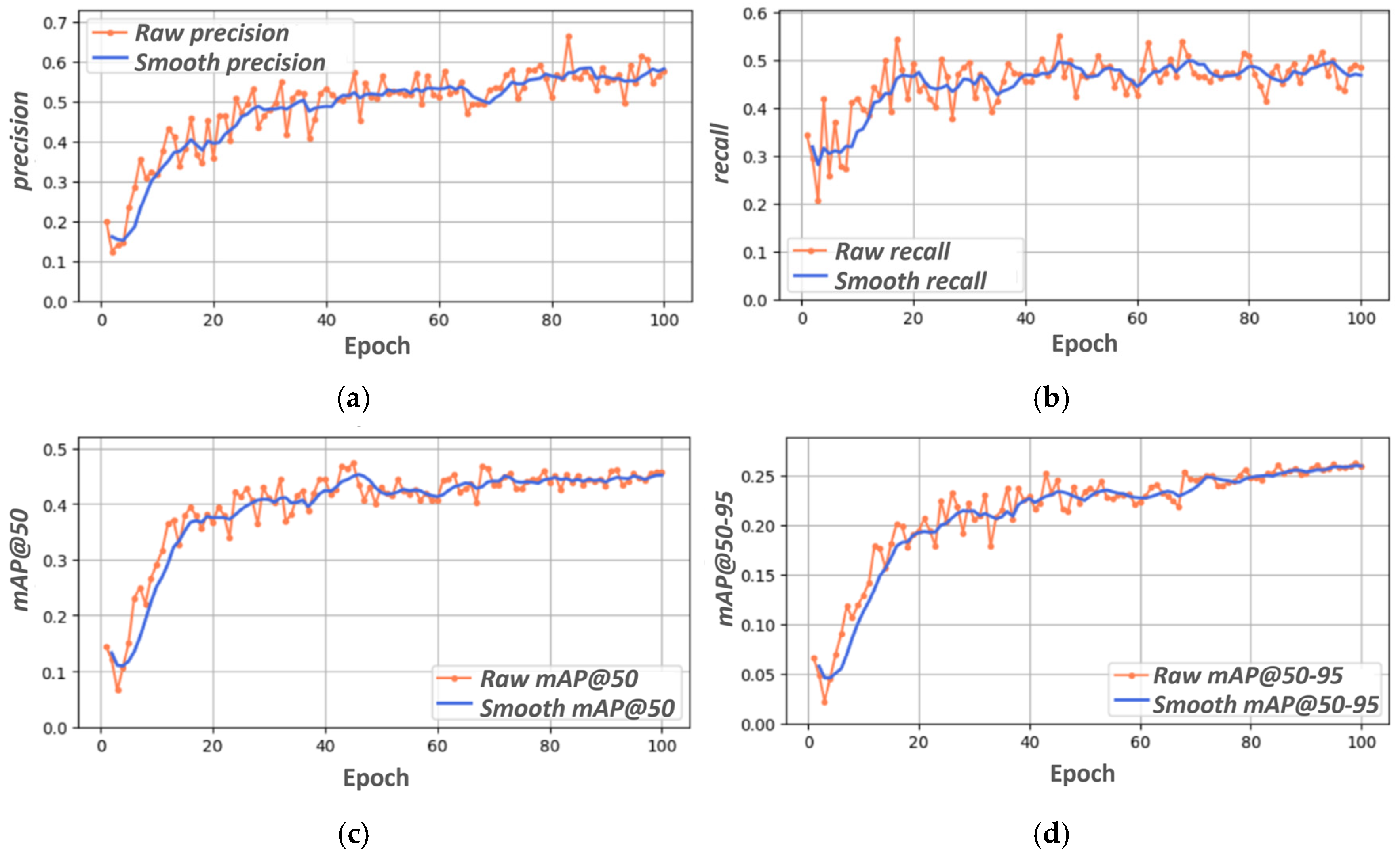
3.1. YOLOV8s Training, Validation, and Testing

Implementation of YOLOv8s for detecting Kudzu plants in GSV images produces promising results, showcasing both accuracy and speed, making it suitable for monitoring applications. Since YOLOv8 was originally trained on the COCO dataset, which includes 91 object categories [57], additional fine-tuning on a custom Kudzu dataset was necessary to enable effective detection. The training and validation metrics over 100 epochs was conducted covering the fine-tuning and also its learning progress.

Training metrics revealed a steady improvement in model performance, which can be seen in Figure 3. The box loss (Figure 3a) gradually decreases over epochs, indicating that our fine-tuned model was improving its ability to refine bounding boxes. The classification loss (Figure 3b) also steadily declines, suggesting enhanced classification performance as training progresses. Similarly, the distribution focal loss (DFL) (Figure 3c) reduces over time, implying improved bounding box predictions and convergence of the model.

In Figure 4, validation loss plots demonstrate the model’s generalization performance. The box loss (Figure 4a) starts with a high value but decreases over less than 20 epochs, eventually stabilizing with some fluctuations. This result suggests that while the model generalizes well, further fine-tuning might be necessary. The classification loss (Figure 4b) follows a similar trajectory, initially spiking before significantly reducing, mirroring the trend observed in the training loss. Likewise, the DFL loss (Figure 4c) decreases over time but stabilizes after 100 epochs, which could indicate potential areas for optimization. All three functions stabilize within a range of 1.5 to 2, which, while not approaching zero, remains acceptable given the challenge of precisely detecting bounding boxes in vegetation. This difficulty arises due to the lack of distinct edges, making exact localization inherently complex.

In terms of detection performance, the two plots in the top row of Figure 5 illustrate the precision and recall metrics. The precision (Figure 5a) steadily increases with fluctuations, indicating that the model is improving in correctly identifying objects while reducing false positives. The recall (Figure 5b) also exhibits an upward trend but with noticeable variability, suggesting there is still room for improvement in detecting all relevant instances. The bottom row depicts the mAP metrics at different thresholds. The mAP@50 (Figure 5c) shows a clear increasing trend, confirming that the model is improving its ability to detect objects with high intersection over union (IoU) thresholds. The mAP@50–95 (Figure 5d), a stricter metric, follows a similar pattern but at a slower rate, reflecting the model’s ability to detect objects with varying overlap thresholds.

The best performance of the YOLOv8s model on the test set is summarized in

Table 1. Values of best performance of the YOLOv8s model for each metric on the test set.

Metric	Value
precision	0.564
recall	0.488
mAP@50	0.458
mAP@50–95	0.263

. The model achieved high precision and recall, with a mAP at IoU threshold 0.5 (mAP@50) of 0.458 and a stricter mAP@50–95 of 0.263, indicating a robust detection capability under varying conditions.

Overall, YOLOv8s was effective in learning and generalizing to unseen data, making it a promising tool for Kudzu plant detection in GSV images. The observed trends, including decreasing losses and increasing precision, recall, and mAP values, confirm the model’s learning effectiveness. However, fluctuations in validation losses suggest that additional tuning could further enhance the model’s performance. These fluctuations may be attributed to several factors. First, the relatively small size of the dataset (432 annotated images) makes the model more sensitive to difficult or ambiguous samples. Prior work shows that models trained on fewer than 1000 images often perform poorly, with more false positives [47]. By comparison, YOLO studies typically use 900–4500 images [44,45,46,47], which reinforces the limitations faced here. Additionally, visual ambiguity in GSV imagery—such as lighting variability, occlusions, and instances where the Kudzu appears distant or only partially visible—can make consistent detection more challenging. This limitation has also been observed in similar studies [47]. Finally, the visual similarity between Kudzu and surrounding vegetation—especially since Kudzu often overtakes existing plant life [82]—can cause confusion in detection, as the model may struggle to distinguish Kudzu from the background in densely vegetated areas.

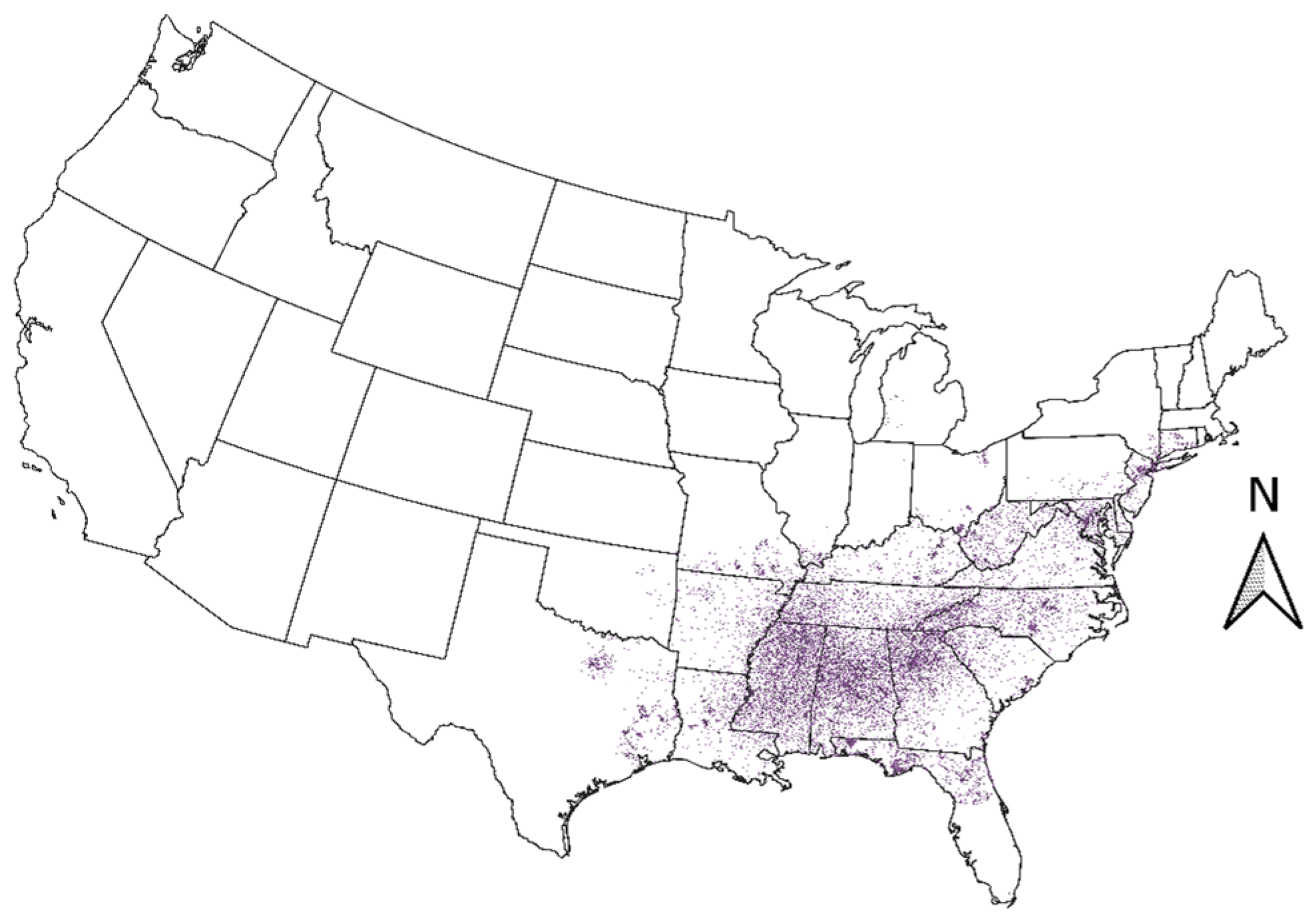
3.2. Geospatial Data for Kudzu in the Conterminous United States

Kudzu GPS locations (Figure 6), according to the latest report (accessed on January 2024), are displayed using QGIS [83]. It was found that Kudzu was more often found in the eastern side of the conterminous United States, with a high frequency of observations for the states of Georgia, Tennessee, Mississippi, and Alabama.

Kudzu Image Dataset Retrieval

GSV images corresponding to Kudzu locations were retrieved using the Google Maps Platform API, which provides metadata on Street View panoramas to determine image availability at specific locations. Only images with a status of ‘OK’ (available) were downloaded. Retrieved images exhibited variations in viewing angles, lighting conditions, and potential obstructions, including road barriers, surrounding vegetation, and unexpected obstacles. Additionally, the Kudzu was captured in different physiological growth stages (Figure 7). Out of the expected 112,376 images, only 41,956 were successfully downloaded, as the remaining 70,420 lacked available imagery at any of the four angles.

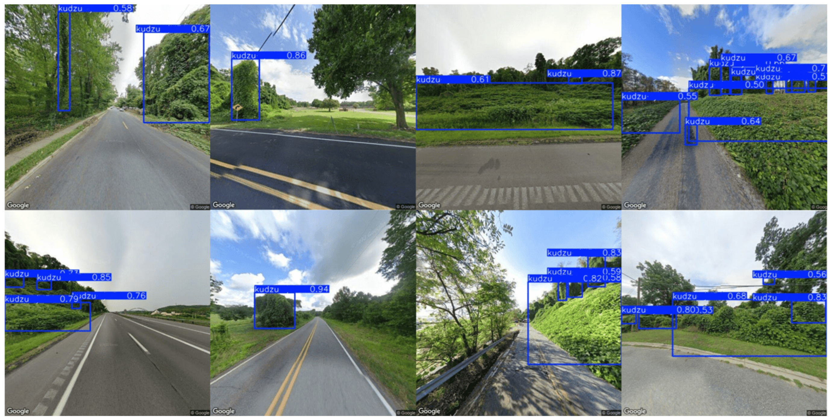
3.3. YOLOv8s Applied to GSV Images

Out of 41,956 GSV images, the YOLOv8s model identified Kudzu instances with a confidence score exceeding 50% in 11,028 images, which corresponded to 6321 GPS locations. We further found that Kudzu instances were available in one, two, three, and four directions in 3083, 2032, 943, and 263 GPS locations, respectively. As an example, Figure 8 displays eight of these Kudzu detections from various perspectives and environments, such as highways or vegetation-covered areas, even in diverse lighting and background conditions.

4. Discussion

Our proposed two-stage data workflow for detecting Kudzu using geospatial data and GSV images offers a scalable solution for invasive species detection, particularly in roadside environments, where traditional remote sensing methods may face limitations due to spatial resolution or computational demands.

One notable workflow capability is its efficiency in data acquisition and processing. The use of GSV images enables rapid and cost-effective data collection over large areas without requiring extensive field campaigns. This advantage stands out when compared to satellite- or UAV-based methods, which often involve significant costs and resources for data acquisition and preprocessing areas [10,27].

Our workflow also excels in its adaptability to small and dispersed areas. Unlike large-scale remote sensing approaches that often overlook small patches of invasive species [12,84], this workflow effectively targets localized roadside environments where Kudzu is commonly found. Additionally, this workflow benefits from the integration of geospatial data. By incorporating geospatial indicators from the INHABIT aggregated occurrence dataset, it ensures accurate historical observations that enable precise identification of AOI. This integration minimizes the risk of analyzing irrelevant regions, a challenge noted in broader-scale studies [11].

Despite its strengths, this workflow has several limitations. One is its dependence on the update of GSV images, as the success of this approach relies heavily on the periodicity and coverage of GSV updates. The Google Maps Platform does not provide a fixed update schedule for Street View [85], and imagery can range from a few months to several years old depending on location. Based on the capture dates of the images utilized in this study, the available imagery spans from 2007 to 2025, with 2023 and 2024 representing the years with the highest frequency of images. This highlights the variability in update frequency across different regions. The complete distribution of available imagery over the years can be found in Appendix B, Figure 1.

Approximately 70,420 images were unavailable due to missing imagery at specific GPS locations, limiting the comprehensiveness of the analysis at inaccessible locations. This challenge has also been reported in other studies utilizing GSV data for environmental monitoring [18]. Additionally, because the model is trained to recognize Kudzu based on its dense foliage, GSV imagery captured during the plant’s off-season—when it appears as bare stems—may result in missed detections. This highlights a temporal limitation tied to the timing of image capture.

While acknowledging the limitations of relying exclusively on GSV data, integrating alternative or complementary data sources presents significant practical challenges. For instance, UAV imagery, while offering ultra-high resolution, is constrained by limited spatial coverage, regulatory restrictions, and the logistical demands of operating flights. Sentinel-2 time-series data, although globally available and regularly updated, lacks the spatial resolution required to detect vegetation such as Kudzu along narrow roadsides, especially in small or dispersed patches. Finally, citizen science platforms depend heavily on voluntary participation and data validation, leading to uneven geographic coverage and limited control over data quality. Therefore, while these sources may be explored in specific contexts, their integration into a scalable and automated pipeline requires incorporation of additional computational tools.

Another limitation is the restricted dataset size used for training, which consisted of only 432 annotated images. This limited sample constrains the model’s ability to generalize across variable conditions, such as seasonal changes or extreme weather periods. Although data augmentation was applied to increase dataset variability, the relatively small size of the training set heightens the risk of overfitting. Future work should prioritize expanding the dataset to enhance robustness, as studies utilizing larger training sets have demonstrated improved generalization and performance [45,46]. However, it is important to note that many of those studies target broad vegetation types or multiple species simultaneously and often use pre-existing large datasets. In contrast, our study focuses specifically on Kudzu detection and required building a custom dataset—a common constraint in early-stage ecological monitoring research. Despite the limited dataset size, our workflow was designed to be scalable. Once the initial model is trained, it can be used to detect additional Kudzu instances, which can then be manually validated and added back into the training set. This iterative, snowball-style process allows for progressive dataset expansion and model improvement without requiring massive initial data collection efforts.

Moreover, while a fixed image resolution of 512 × 512 pixels in YOLOv8s enables faster processing [61], it may also lead to information loss. Downsizing images could make smaller Kudzu instances undetectable, presenting a challenge for accurate detection. Finally, our workflow’s reliance on static GSV imagery introduces a limitation in temporal analysis. GSV images do not allow for monitoring the growth or spread of Kudzu over time. In contrast, satellite-based methods, such as those utilizing Sentinel-2 or AVIRIS data, enable temporal analyses but compromise spatial resolution when focusing on small areas [10].

Compared to other methods for invasive species detection, this workflow balances efficiency and precision by targeting specific AOIs with high-resolution imagery while applying advanced object detection algorithms. Having demonstrated the feasibility of this pipeline, it can now be applied to other geographic areas and adapted for the detection and monitoring of additional species. Nevertheless, further research opportunities remain to be explored. First, expanding the dataset size and incorporating additional image sources, such as UAVs or satellite imagery, could enhance both the robustness and generalizability of the model. Second, addressing temporal limitations is essential to improve the workflow’s suitability for long-term monitoring efforts. Third, improving spatial coverage estimation is warranted, as GSV imagery typically provides perpendicular shots relative to the ground; however, terrain variability—including slopes and obstructions—can restrict the effective surface area captured in each image. Future studies may benefit from integrating GPS data with LiDAR or photogrammetry to more accurately quantify the ground area represented in each image. Additionally, enhancements to scanning protocols are recommended. Rather than relying exclusively on existing GSV images at fixed GPS coordinates, targeted field campaigns could be designed to systematically capture roadside imagery at regular intervals and angles along the road network, thereby ensuring more comprehensive coverage of the target areas. Collectively, these advancements would not only refine detection accuracy but also empower invasive species managers to prioritize interventions based on spatially explicit, time-stamped data.

5. Conclusions

This study presents a two-stage data workflow that integrates geospatial data and GSV imagery to efficiently and accurately detect Kudzu vines in small and dispersed areas, particularly along roadsides. Using historical observations aggregated by INHABIT to define AOIs and applying the YOLOv8s object detection model for image analysis, this approach becomes a potential resource for invasive species monitoring. Our results highlight the effectiveness of this workflow in addressing challenges associated with traditional remote sensing methods, such as high computational demands and limited resolution for small-scale detection. The YOLOv8s model achieved high precision and mean average precision (mAP), showcasing its ability to identify Kudzu under diverse environmental conditions. Additionally, the use of GSV images facilitated cost-effective data collection over large areas, making this approach scalable and adaptable for extensive monitoring efforts. However, this study also identifies several limitations that constrain its broader applicability. The reliance on GSV imagery introduces challenges related to incomplete geographic coverage and outdated imagery, limiting temporal analysis of Kudzu growth and spread. Furthermore, the relatively small training dataset restricts the model’s ability to generalize across varying environmental conditions, such as seasonal changes or extreme weather. While data augmentation partially mitigates this issue, larger and more diverse datasets are necessary to enhance model robustness. Future research should focus on addressing these limitations by expanding the dataset, incorporating diverse image sources, improving spatial and temporal coverage, and refining image acquisition protocols, which will further enhance the workflow’s accuracy and practical utility for invasive species monitoring and management.

References

1. Kohli, R.K. Alien—Plant Invasion in the Anthropocene How Does an Alien Plant Become. Anthr. Sci. 2024, 2, 177–179. [Google Scholar] [CrossRef]
2. Tonini, F.; Shoemaker, D.; Petrasova, A.; Harmon, B.; Petras, V.; Cobb, R.C.; Mitasova, H.; Meentemeyer, R.K. Tangible geospatial modeling for collaborative solutions to invasive species management. Environ. Model. Softw. 2017, 92, 176–188. [Google Scholar] [CrossRef]
3. Lee, J.G.; Kang, M. Geospatial Big Data: Challenges and Opportunities. Big Data Res. 2015, 2, 74–81. [Google Scholar] [CrossRef]
4. Young, N.E.; Jarnevich, C.S.; Sofaer, H.R.; Pearse, I.; Sullivan, J.; Engelstad, P.; Stohlgren, T.J. A modeling workflow that balances automation and human intervention to inform invasive plant management decisions at multiple spatial scales. PLoS ONE 2020, 15, e0229253. [Google Scholar] [CrossRef]
5. Valavi, R.; Guillera-Arroita, G.; Lahoz-Monfort, J.J.; Elith, J. Predictive performance of presence-only species distribution models: A benchmark study with reproducible code. Ecol. Monogr. 2022, 92, e01486. [Google Scholar] [CrossRef]
6. Callen, S.T.; Miller, A.J. Signatures of niche conservatism and niche shift in the North American kudzu (Pueraria montana) invasion. Divers. Distrib. 2015, 21, 853–863. [Google Scholar] [CrossRef]
7. Bradley, B.A.; Wilcove, D.S.; Oppenheimer, M. Climate change increases risk of plant invasion in the Eastern United States. Biol. Invasions 2010, 12, 1855–1872. [Google Scholar] [CrossRef]
8. Evans, A.E.; Jarnevich, C.S.; Beaury, E.M.; Engelstad, P.S.; Teich, N.B.; LaRoe, J.M.; Bradley, B.A. Shifting hotspots: Climate change projected to drive contractions and expansions of invasive plant abundance habitats. Divers. Distrib. 2024, 30, 41–54. [Google Scholar] [CrossRef]
9. Hoffberg, S.L.; Mauricio, R. The persistence of invasive populations of kudzu near the northern periphery of its range in New York City determined from historical data. J. Torrey Bot. Soc. 2016, 143, 437–442. [Google Scholar] [CrossRef]
10. Jensen, T.; Hass, F.S.; Akbar, M.S.; Petersen, P.H.; Arsanjani, J.J. Employing machine learning for detection of invasive species using sentinel-2 and aviris data: The case of Kudzu in the United States. Sustainability 2020, 12, 3544. [Google Scholar] [CrossRef]
11. Liang, W.; Abidi, M.; Carrasco, L.; McNelis, J.; Tran, L.; Li, Y.; Grant, J. Mapping vegetation at species level with high-resolution multispectral and lidar data over a large spatial area: A case study with Kudzu. Remote Sens. 2020, 12, 609. [Google Scholar] [CrossRef]
12. Meyer, M.d.F.; Gonçalves, J.A.; Cunha, J.F.R.; Ramos, S.C.d.C.e.S.; Bio, A.M.F. Application of a Multispectral UAS to Assess the Cover and Biomass of the Invasive Dune Species Carpobrotus edulis. Remote Sens. 2023, 15, 2411. [Google Scholar] [CrossRef]
13. Xu, Z.; Hu, H.; Wang, T.; Zhao, Y.; Zhou, C.; Xu, H.; Mao, X. Identification of growth years of Kudzu root by hyperspectral imaging combined with spectral–spatial feature tokenization transformer. Comput. Electron. Agric. 2023, 214, 108332. [Google Scholar] [CrossRef]
14. Kotowska, D.; Pärt, T.; Żmihorski, M. Evaluating Google Street View for tracking invasive alien plants along roads. Ecol. Indic. 2021, 121, 107020. [Google Scholar] [CrossRef]
15. Nesse, K.; Airt, L. How Useful Is GSV As an Environmental Observation Tool? An Analysis of the Evidence So Far. SSRN Electron. J. 2017. [Google Scholar] [CrossRef]
16. Rousselet, J.; Imbert, C.-E.; Dekri, A.; Garcia, J.; Goussard, F.; Vincent, B.; Denux, O.; Robinet, C.; Dorkeld, F.; Roques, A.; et al. Assessing Species Distribution Using Google Street View: A Pilot Study with the Pine Processionary Moth. PLoS ONE 2013, 8, e74918. [Google Scholar] [CrossRef] [PubMed]
17. Pardo-Primoy, D.; Fagúndez, J. Assessment of the distribution and recent spread of the invasive grass Cortaderia selloana in Industrial Sites in Galicia, NW Spain. Flora 2019, 259, 151465. [Google Scholar] [CrossRef]
18. Perrett, A.; Pollard, H.; Barnes, C.; Schofield, M.; Qie, L.; Bosilj, P.; Brown, J.M. DeepVerge: Classification of roadside verge biodiversity and conservation potential. Comput. Environ. Urban Syst. 2023, 102, 101968. [Google Scholar] [CrossRef]
19. Shen, M.; Tang, M.; Jiao, W.; Li, Y. Kudzu invasion and its influential factors in the southeastern United States. Int. J. Appl. Earth Obs. Geoinf. 2024, 130, 103872. [Google Scholar] [CrossRef]
20. Jarnevich, C.S.; LaRoe, J.; Engelstad, P.; Hays, B.; Henderson, G.; Williams, D.; Shadwell, K.; Pearse, I.S.; Prevey, J.S.; Sofaer, H.R. INHABIT Species Potential Distribution Across the Contiguous United States; Version 3.0; U.S. Geological Survey Data Release; U.S. Geological Survey: Reston, VA, USA, 2023. [CrossRef]
21. Zaka, M.M.; Samat, A. Advances in Remote Sensing and Machine Learning Methods for Invasive Plants Study: A Comprehensive Review. Remote Sens. 2024, 16, 3781. [Google Scholar] [CrossRef]
22. Kaya, A.; Seydi, A.; Catal, C.; Yalin, H.; Temucin, H. Analysis of transfer learning for deep neural network based plant classification models. Comput. Electron. Agric. 2019, 158, 20–29. [Google Scholar] [CrossRef]
23. Lecun, Y.; Bengio, Y.; Hinton, G. Deep learning. Nature 2015, 521, 436–444. [Google Scholar] [CrossRef] [PubMed]
24. Wang, H.; Czerminski, R.; Jamieson, A.C. Neural Networks and Deep Learning. In The Machine Age of Customer Insight; Emerald Publishing Limited: Leeds, UK, 2021; pp. 91–101. [Google Scholar] [CrossRef]
25. Alzubaidi, L.; Zhang, J.; Humaidi, A.J.; Al-Dujaili, A.; Duan, Y.; Al-Shamma, O.; Santamaría, J.; Fadhel, M.A.; Al-Amidie, M.; Farhan, L. Review of deep learning: Concepts, CNN architectures, challenges, applications, future directions. J. Big Data 2021, 8, 53. [Google Scholar] [CrossRef]
26. Cohen, J.G.; Lewis, M.J. Development of an Automated Monitoring Platform for Invasive Plants in a Rare Great Lakes Ecosystem Using Uncrewed Aerial Systems and Convolutional Neural Networks. In Proceedings of the 2020 International Conference on Unmanned Aircraft Systems (ICUAS), Athens, Greece, 1–4 September 2020; pp. 1553–1564. [Google Scholar] [CrossRef]
27. Kattenborn, T.; Eichel, J.; Schmidtlein, S.; Wiser, S.; Burrows, L.; Fassnacht, F.E. Convolutional Neural Networks accurately predict cover fractions of plant species and communities in Unmanned Aerial Vehicle imagery. Remote Sens. Ecol. Conserv. 2020, 6, 472–486. [Google Scholar] [CrossRef]
28. Kun, X.; Wei, W.; Sun, Y.; Wang, Y.; Xin, Q. Mapping fine-spatial-resolution vegetation spring phenology from individual Landsat images using a convolutional neural network. Int. J. Remote Sens. 2023, 44, 3059–3081. [Google Scholar] [CrossRef]
29. Shen, M.; Tang, M.; Li, Y. Phenology and spectral unmixing-based invasive kudzu mapping: A case study in knox county, tennessee. Remote Sens. 2021, 13, 4551. [Google Scholar] [CrossRef]
30. Zhou, X.; Xin, Q.; Dai, Y.; Li, W. A deep-learning-based experiment for benchmarking the performance of global terrestrial vegetation phenology models. Glonal Ecol. Biogeogr. 2021, 30, 2178–2199. [Google Scholar] [CrossRef]
31. Lake, T.A.; Runquist, R.D.B.; Moeller, D.A. Deep learning detects invasive plant species across complex landscapes using Worldview-2 and Planetscope satellite imagery. Remote Sens. Ecol. Conserv. 2022, 8, 875–889. [Google Scholar] [CrossRef]
32. Kattenborn, T.; Leitloff, J.; Schiefer, F.; Hinz, S. Review on Convolutional Neural Networks (CNN) in vegetation remote sensing. ISPRS J. Photogramm. Remote Sens. 2021, 173, 24–49. [Google Scholar] [CrossRef]
33. Tang, F.; Zhang, D.; Zhao, X. Efficiently deep learning for monitoring Ipomoea cairica (L.) sweets in the wild. Math. Biosci. Eng. 2021, 18, 1121–1135. [Google Scholar] [CrossRef]
34. Qiao, X.; Li, Y.-Z.; Su, G.-Y.; Tian, H.-K.; Zhang, S.; Sun, Z.-Y.; Yang, L.; Wan, F.-H.; Qian, W.-Q. MmNet: Identifying Mikania micrantha Kunth in the wild via a deep Convolutional Neural Network. J. Integr. Agric. 2020, 19, 1292–1300. [Google Scholar] [CrossRef]
35. Zhong, H.; Zhang, Z.; Liu, H.; Wu, J.; Lin, W. Individual Tree Species Identification for Complex Coniferous and Broad-Leaved Mixed Forests Based on Deep Learning Combined with UAV LiDAR Data and RGB Images. Forests 2024, 15, 293. [Google Scholar] [CrossRef]
36. Deneu, B.; Servajean, M.; Bonnet, P.; Botella, C.; Munoz, F.; Joly, A. Convolutional neural networks improve species distribution modelling by capturing the spatial structure of the environment. PLoS Comput. Biol. 2021, 17, e1008856. [Google Scholar] [CrossRef] [PubMed]
37. Botella, C.; Joly, A.; Bonnet, P. Species distribution modeling based on the automated identification of citizen observations. Appl. Plant Sci. 2018, 6, e1029. [Google Scholar] [CrossRef]
38. Sermanet, P.; Eigen, D.; Zhang, X.; Mathieu, M.; Fergus, R.; LeCun, Y. OverFeat: Integrated Recognition, Localization and Detection using Convolutional Networks. In Proceedings of the 2nd International Conference on Learning Representations, ICLR 2014—Conference Track Proceedings, Banff, AB, Canada, 14–16 April 2013. [Google Scholar]
39. Ren, S.; He, K.; Girshick, R.; Sun, J. Faster R-CNN: Towards Real-Time Object Detection with Region Proposal Networks. IEEE Trans. Pattern Anal. Mach. Intell. 2015, 39, 1137–1149. [Google Scholar] [CrossRef]
40. Redmon, J.; Divvala, S.; Girshick, R.; Farhadi, A. You Only Look Once: Unified, Real-Time Object Detection. In Proceedings of the IEEE Computer Society Conference on Computer Vision and Pattern Recognition, Las Vegas, NV, USA, 27–30 June 2016; pp. 779–788. [Google Scholar] [CrossRef]
41. Liu, W.; Anguelov, D.; Erhan, D.; Szegedy, C.; Reed, S.; Fu, C.Y.; Berg, A.C. SSD: Single Shot MultiBox Detector. In Proceedings of the European Conference on Computer Vision, Amsterdam, The Netherlands, 11–14 October 2016. [Google Scholar] [CrossRef]
42. Dalal, N.; Triggs, B. Histograms of oriented gradients for human detection. In Proceedings of the Computer Vision and Pattern Recognition, San Diego, CA, USA, 20–26 June 2005; pp. 886–893. [Google Scholar] [CrossRef]
43. Lowe, D.G. Object recognition from local scale-invariant features. In Proceedings of the IEEE International Conference on Computer Vision, Kerkyra, Greece, 20–27 September 1999; Volume 2, pp. 1150–1157. [Google Scholar] [CrossRef]
44. Zhen, T. Integrating Deep Learning and Google Street View for Novel Weed Mapping. Master’s Thesis, UC Davis, Davis, CA, USA, 2022. Available online: https://escholarship.org/uc/item/8pd05123 (accessed on 20 January 2025).
45. Salahin, S.M.T.U.; Mehnaz, F.; Zaman, A.; Barua, K.; Mahbub, D.M.S. Detecting and Mapping of Roadside Trees from Google Street View. SSRN Electron. J. 2024. [Google Scholar] [CrossRef]
46. Velasquez-Camacho, L.; Etxegarai, M.; de-Miguel, S. Implementing Deep Learning algorithms for urban tree detection and geolocation with high-resolution aerial, satellite, and ground-level images. Comput. Environ. Urban Syst. 2023, 105, 102025. [Google Scholar] [CrossRef]
47. Gautam, D.; Mawardi, Z.; Elliott, L.; Loewensteiner, D.; Whiteside, T.; Brooks, S. Detection of Invasive Species (Siam Weed) Using Drone-Based Imaging and YOLO Deep Learning Model. Remote Sens. 2025, 17, 120. [Google Scholar] [CrossRef]
48. Terven, J.; Córdova-Esparza, D.M.; Romero-González, J.A. A Comprehensive Review of YOLO Architectures in Computer Vision: From YOLOv1 to YOLOv8 and YOLO-NAS. Mach. Learn. Knowl. Extr. 2023, 5, 1680–1716. [Google Scholar] [CrossRef]
49. Yaseen, M. What Is YOLOv8: An In-Depth Exploration of the Internal Features of the Next-Generation Object Detector. arXiv 2024, arXiv:2408.15857. Available online: http://arxiv.org/abs/2408.15857 (accessed on 25 February 2025).
50. Haritha, I.V.S.L.; Harshini, M.; Patil, S.; Philip, J. Real Time Object Detection using YOLO Algorithm. In Proceedings of the 6th International Conference on Electronics, Communication and Aerospace Technology, ICECA 2022—Proceedings, Coimbatore, India, 1–3 December 2022; pp. 1465–1468. [Google Scholar] [CrossRef]
51. Aboyomi, D.D.; Daniel, C. A Comparative Analysis of Modern Object Detection Algorithms: YOLO vs. SSD vs. Faster R-CNN. ITEJ Inf. Technol. Eng. J. 2023, 8, 96–106. [Google Scholar] [CrossRef]
52. Li, M.; Zhang, Z.; Lei, L.; Wang, X.; Guo, X. Agricultural Greenhouses Detection in High-Resolution Satellite Images Based on Convolutional Neural Networks: Comparison of Faster R-CNN, YOLO v3 and SSD. Sensors 2020, 20, 4938. [Google Scholar] [CrossRef]
53. Tan, L.; Huangfu, T.; Wu, L.; Chen, W. Comparison of YOLO v3, Faster R-CNN, and SSD for Real-Time Pill Identification. Preprint 2021. Available online: https://www.researchsquare.com/article/rs-668895/v1 (accessed on 22 April 2025).
54. Sanchez, S.A.; Romero, H.J.; Morales, A.D. A review: Comparison of performance metrics of pretrained models for object detection using the TensorFlow framework. IOP Conf. Ser. Mater. Sci. Eng. 2020, 844, 012024. [Google Scholar] [CrossRef]
55. Jocher, G.; Qiu, J.; Chaurasia, A. Ultralytics YOLO; Version 8.0.0; Ultralytics: Frederick, MD, USA, 2023. [Google Scholar]
56. Li, R.; He, Y.; Li, Y.; Qin, W.; Abbas, A.; Ji, R.; Li, S.; Wu, Y.; Sun, X.; Yang, J. Identification of cotton pest and disease based on CFNet-VoV-GCSP-LSKNet-YOLOv8s: A new era of precision agriculture. Front. Plant Sci. 2024, 15, 1348402. [Google Scholar] [CrossRef] [PubMed]
57. Lin, T.-Y.; Maire, M.; Belongie, S.; Hays, J.; Perona, P.; Ramanan, D.; Dollár, P.; Zitnick, C.L. Microsoft COCO: Common Objects in Context. In Computer Vision—ECCV 2014: 13th European Conference, Zurich, Switzerland, 6–12 September 2014, Proceedings, Part V; Springer: Cham, Switzerland; pp. 740–755. [CrossRef]
58. Wang, G.; Chen, Y.; An, P.; Hong, H.; Hu, J.; Huang, T. UAV-YOLOv8: A Small-Object-Detection Model Based on Improved YOLOv8 for UAV Aerial Photography Scenarios. Sensors 2023, 23, 7190. [Google Scholar] [CrossRef] [PubMed]
59. Abdullah, A.; Amran, G.A.; Tahmid, S.M.A.; Alabrah, A.; AL-Bakhrani, A.A.; Ali, A. A Deep-Learning-Based Model for the Detection of Diseased Tomato Leaves. Agronomy 2024, 14, 1593. [Google Scholar] [CrossRef]
60. Wang, Y.; Yi, C.; Huang, T.; Liu, J. Research on Intelligent Recognition for Plant Pests and Diseases Based on Improved YOLOv8 Model. Appl. Sci. 2024, 14, 5353. [Google Scholar] [CrossRef]
61. Ahmed, S.; Revolinski, S.R.; Maughan, P.W.; Savic, M.; Kalin, J.; Burke, I.C. Deep learning–based detection and quantification of weed seed mixtures. Weed Sci. 2024, 72, 655–663. [Google Scholar] [CrossRef]
62. Diao, Z.; Ma, S.; Zhang, D.; Zhang, J.; Guo, P.; He, Z.; Zhao, S.; Zhang, B. Algorithm for Corn Crop Row Recognition during Different Growth Stages Based on ST-YOLOv8s Network. Agronomy 2024, 14, 1466. [Google Scholar] [CrossRef]
63. Venverloo, T.; Duarte, F. Towards real-time monitoring of insect species populations. Sci. Rep. 2024, 14, 18727. [Google Scholar] [CrossRef] [PubMed]
64. Kathir, M.; Balaji, V.; Ashwini, K. Animal Intrusion Detection Using Yolo V8. In Proceedings of the 2024 10th International Conference on Advanced Computing and Communication Systems (ICACCS), Coimbatore, India, 14–15 March 2024; Volume 1, pp. 206–211. [Google Scholar] [CrossRef]
65. Dwyer, B.; Nelson, J.; Hansen, T. Roboflow, Version 1.0. 2024. Available online: https://roboflow.com (accessed on 25 February 2025).
66. Shahinfar, S.; Meek, P.; Falzon, G. ‘How many images do I need?’ Understanding how sample size per class affects deep learning model performance metrics for balanced designs in autonomous wildlife monitoring. Ecol. Inform. 2020, 57, 101085. [Google Scholar] [CrossRef]
67. Bullock, J.; Cuesta-Lazaro, C.; Quera-Bofarull, A. XNet: A convolutional neural network (CNN) implementation for medical X-Ray image segmentation suitable for small datasets. In Proceedings of the SPIE 10953, Medical Imaging 2019: Biomedical Applications in Molecular, Structural, and Functional Imaging, San Diego, CA, USA, 19–21 February 2019. [Google Scholar] [CrossRef]
68. Foroughi, F.; Chen, Z.; Wang, J. A CNN-Based System for Mobile Robot Navigation in Indoor Environments via Visual Localization with a Small Dataset. World Electr. Veh. J. 2021, 12, 134. [Google Scholar] [CrossRef]
69. Gholamy, A.; Kreinovich, V.; Kosheleva, O. Why 70/30 or 80/20 Relation Between Training and Testing Sets: A Pedagogical Explanation. Departmental Technical Reports (CS). 2018. Available online: https://scholarworks.utep.edu/cs_techrep/1209 (accessed on 25 February 2025).
70. Zhao, Y.; Zou, Y.; Wang, L.; Su, R.; He, Q.; Jiang, K.; Chen, B.; Xing, Y.; Liu, T.; Zhang, H.; et al. Tropical Rainforest Successional Processes can Facilitate Successfully Recovery of Extremely Degraded Tropical Forest Ecosystems Following Intensive Mining Operations. Front. Environ. Sci. 2021, 9, 701210. [Google Scholar] [CrossRef]
71. EDDMapS. Early Detection & Distribution Mapping System. The University of Georgia—Center for Invasive Species and Ecosystem Health. Available online: http://www.eddmaps.org/ (accessed on 25 February 2025).
72. Ali, A.H.; Abdulazeez, A.M. Transfer Learning in Machine Learning: A Review of Methods and Applications. Indones. J. Comput. Sci. 2024, 13, 4227–4259. [Google Scholar] [CrossRef]
73. Zhang, Y.F.; Ren, W.; Zhang, Z.; Jia, Z.; Wang, L.; Tan, T. Focal and Efficient IOU Loss for Accurate Bounding Box Regression. Neurocomputing 2021, 506, 146–157. [Google Scholar] [CrossRef]
74. Charoenphakdee, N.; Vongkulbhisal, J.; Chairatanakul, N.; Sugiyama, M. On Focal Loss for Class-Posterior Probability Estimation: A Theoretical Perspective. In Proceedings of the IEEE Computer Society Conference on Computer Vision and Pattern Recognition, Seattle, WA, USA, 14–19 June 2020; pp. 5198–5207. [Google Scholar] [CrossRef]
75. Li, X.; Lv, C.; Wang, W.; Li, G.; Yang, L.; Yang, J. Generalized Focal Loss: Towards Efficient Representation Learning for Dense Object Detection. IEEE Trans. Pattern Anal. Mach. Intell. 2023, 45, 3139–3153. [Google Scholar] [CrossRef]
76. Maxwell, A.E.; Warner, T.A.; Guillén, L.A. Accuracy Assessment in Convolutional Neural Network-Based Deep Learning Remote Sensing Studies—Part 1: Literature Review. Remote Sens. 2021, 13, 2450. [Google Scholar] [CrossRef]
77. Ozenne, B.; Subtil, F.; Maucort-Boulch, D. The precision--recall curve overcame the optimism of the receiver operating characteristic curve in rare diseases. J. Clin. Epidemiol. 2015, 68, 855–859. [Google Scholar] [CrossRef]
78. Powers, D.M.W. Evaluation: From Precision, Recall and F-Measure to ROC, Informedness, Markedness and Correlation. arxiv 2020, arXiv:2010.16061. Available online: https://arxiv.org/abs/2010.16061v1 (accessed on 25 February 2025).
79. Olson, D.L.; Delen, D. Advanced data mining techniques. In Advanced Data Mining Techniques; Springer Nature: Dordrecht, The Netherlands, 2008; pp. 1–180. [Google Scholar] [CrossRef]
80. Sobti, A.; Arora, C.; Balakrishnan, M. Object Detection in Real-Time Systems: Going beyond Precision. In Proceedings of the 2018 IEEE Winter Conference on Applications of Computer Vision, WACV 2018, Lake Tahoe, NV, USA, 12–15 March 2018; pp. 1020–1028. [Google Scholar] [CrossRef]
81. Khow, Z.J.; Tan, Y.F.; Karim, H.A.; Rashid, H.A.A. Improved YOLOv8 Model for a Comprehensive Approach to Object Detection and Distance Estimation. IEEE Access 2024, 12, 63754–63767. [Google Scholar] [CrossRef]
82. Loewenstein, N.J.; Enloe, S.F.; Everest, J.W.; Miller, J.H.; Ball, D.M.; Patterson, M.G. History and Use of Kudzu in the Southeastern United States—Alabama Cooperative Extension System. System ACE. Available online: https://www.aces.edu/blog/topics/forestry-wildlife/the-history-and-use-of-kudzu-in-the-southeastern-united-states/ (accessed on 15 April 2025).
83. QGIS. 2024. Available online: http://qgis.org (accessed on 22 April 2025).
84. Jarnevich, C.S.; Young, N.E.; Thomas, C.C.; Grissom, P.; Backer, D.; Frid, L. Assessing ecological uncertainty and simulation model sensitivity to evaluate an invasive plant species’ potential impacts to the landscape. Sci. Rep. 2020, 10, 19069. [Google Scholar] [CrossRef] [PubMed]
85. Streetview Request and Response|Street View Static API|Google for Developers. Available online: https://developers.google.com/maps/documentation/streetview/request-streetview (accessed on 11 March 2025).
Figure 1. Labeled image used for training: yellow outlines indicate bounding boxes drawn around Kudzu, forming part of the labeled dataset for model training.
Earth 06 00040 g001
Figure 2. Data workflow for Kudzu detection with YOLOv8s. Blue boxes represent the image dataset preparation and model training pipeline mentioned in Section 2.1. Green boxes indicate the location sourcing and image retrieval process explained in Section 2.2. Orange boxes represent the model fine-tuning and application to Google Street View (GSV) images, which can be found in Section 2.3.
Earth 06 00040 g002
Figure 3. Training metrics of the YOLOv8s model: (a) box loss (train/box_loss), (b) classification loss (train/cls_loss), and (c) distribution focal loss (train/dfl_loss).
Earth 06 00040 g003
Figure 4. Validation losses of the YOLO model over 100 epochs: (a) box loss (val/box_loss), (b) classification loss (val/cls_loss), and (c) distribution focal loss (val/dfl_loss).
Earth 06 00040 g004
Figure 5. Model evaluation metrics of the YOLOv8s model over 100 epochs including (a) precision, (b) recall, (c) mean average precision calculated at an intersection over union threshold of 0.50 (mAP@50), and (d) mean average precision calculated at varying intersection over union thresholds, ranging from 0.50 to 0.95 (mAP@50–95). The x-axis showcases the 100 epochs, indicating the progress of the model during training. The y-axis represents the improvement in performance metrics with each epoch, providing insights into the model’s performance throughout the training process.
Earth 06 00040 g005
Figure 6. GPS locations of Kudzu (Pueraria montana) for the conterminous United States. Each purple dot represents a reported Kudzu observation.
Earth 06 00040 g006
Figure 7. Set of Google Street View images showing angles and lightning to capture Kudzu, including physiological stages with immersed neighboring vegetation.
Earth 06 00040 g007
Figure 8. Series of Google Street View images with bounding boxes detecting the Kudzu plant. The images illustrate various locations where Kudzu is identified with blue bounding boxes. Each bounding box is annotated with the label of Kudzu and the confidence score, indicating the model’s certainty in its classification.
Earth 06 00040 g008