Abstract
The Cheremskyi Nature Reserve, situated in the Volyn region of Ukraine, constitutes a pivotal element of the European ecological network, distinguished by its distinctive mosaic of peatlands, bogs, and floodplain forests. This study utilizes Sentinel-2 satellite imagery and the Google Earth Engine (GEE) to assess the spatiotemporal patterns of various vegetation indices (NDVI, EVI, SAVI, MSAVI, GNDVI, NDRE, NDWI) from 2017 to 2024. The study aims to select the most suitable combination of vegetation spectral indices for future research. The analysis reveals significant negative trends in NDVI, SAVI, MSAVI, GNDVI, and NDRE, indicating a decline in vegetation health, while NDWI shows a positive trend, suggesting an increased vegetation water content. Correlation analysis underscores robust interrelationships among the indices, with NDVI and SAVI identified as the most significant through random forest feature importance analysis. Principal component analysis (PCA) further elucidates the primary axes of variability, emphasizing the complex interplay between vegetation greenness and moisture content. The findings underscore the utility of multi-index analyses in enhancing predictive capabilities for ecosystem monitoring and support targeted conservation strategies for the sustainable management of the Cheremskyi Nature Reserve.
1. Introduction
The wetlands and peatlands of Ukrainian Polissya are a key component of the European ecological network, forming unique landscapes that combine forests, bogs, floodplain meadows, and shallow lakes. This region, which stretches across northern Ukraine, is part of the larger Polissya natural complex, which covers the territories of Ukraine, Belarus, Russia, and Poland. The Ukrainian Polissya region is characterized by a high concentration of peat bogs [1], which have accumulated organic matter over thousands of years, making them important carbon reservoirs and an element of global climate regulation. Peatlands also maintain the hydrological balance of the region by acting as natural sponges that absorb excess moisture during floods and gradually release it during droughts [2,3].
Over the past decades, these ecosystems have undergone significant anthropogenic transformations, in particular due to large-scale drainage for agriculture, peat extraction [4], and forestry. According to environmental organizations [5], more than 60% of Ukraine’s peatlands are already drained or degraded, leading to the release of CO2, reduced biodiversity and increased fire risks.
The Cheremskyi Nature Reserve [6], located in the Volyn region, is one of the few refugia with almost intact peatlands typical of the Polissya region. Its ecosystems include lowland and upland bogs, transitional bogs, and adjacent forests, creating a mosaic of environments with high ecological specificity. However, even this area faces threats from climate change (more frequent droughts) and the transboundary impact of drainage systems.
Current research on the wetlands of Ukrainian Polissya remains fragmented [7], focusing mainly on local biotic inventories [8,9,10], while a comprehensive analysis of hydroecological changes using satellite technologies is limited [11].
Remote sensing has emerged as a pivotal technology for assessing wetland health and dynamics, offering spatially explicit, cost-effective, and non-invasive solutions [12,13,14,15,16]. In this context, multispectral indices derived from satellite imagery have become indispensable for quantifying vegetation vitality, water availability, and soil moisture—key parameters for understanding wetland ecosystem functioning.
The Sentinel-2 mission [17], with its high spatial (10–20 m) and temporal (5-day revisit) resolution, provides effective opportunities for monitoring fine-scale changes in heterogeneous wetland environments. Coupled with cloud-based platforms such as Google Earth Engine (GEE) [18], which enables efficient processing of large geospatial datasets, Sentinel-2 imagery facilitates the derivation of spectral indices, like the normalized difference vegetation index (NDVI), enhanced vegetation index (EVI), soil-adjusted vegetation moisture index (SAVI), modified soil-adjusted vegetation moisture index (MSAVI), green normalized difference vegetation index (GNDVI), modified normalized difference water index (MNDWI), normalized difference red-edge index (NDRE), and normalized difference water index (NDWI). These vegetation indices collectively capture the ecological gradients inherent to wetlands, from open water bodies to emergent vegetation and saturated soils.
Despite their widespread application, the interrelationships and synergies between these indices in wetland contexts remain underexplored.
Various studies have shown [19,20,21] that wetlands in different parts of the world require an individual approach to selecting the optimal combinations of spectral indices for their effective study. Furthermore, the Cheremskyi Nature Reserve—a protected wetland of international importance in Ukraine, characterized by its mosaic of marshes, peatlands, and floodplain forests—has yet to be comprehensively analyzed using modern remote sensing approaches. This research gap limits the ability to develop targeted conservation strategies for such ecologically sensitive regions.
This study aims to:
- assess the spatial and temporal patterns of NDVI, EVI, SAVI, MSAVI, GNDVI, NDRE, and NDWI within the Cheremsky Nature Reserve using Sentinel-2 data processed in GEE;
- investigate the relationships between these indices to identify the main drivers of wetland variability;
- investigate which of the indices are most appropriate for the studies of Ukrainian Polissya wetlands.
By integrating multi-index analyses with advanced geospatial tools, this work seeks to advance methodological frameworks for wetland assessment while providing actionable insights for the sustainable management of the Cheremskyi Nature Reserve and analogous ecosystems in Ukrainian Polissya.
2. Materials and Methods
2.1. Study Region
Cheremsky Nature Reserve is the only nature reserve in the Volyn region and one of the northernmost in Ukraine. It was established by Presidential Decree No. 1234 of 19 December 2001 [22] on the basis of the Cheremsky Reserve of national importance with an area of 903 hectares and its protection zone, as well as 3 reserves of local importance: the ornithological reserve ‘Suzanka tract’, the general zoological reserve ‘Karasynsky’ and the botanical reserve ‘Karasynsky spruce-1’. The total area of the reserve is 2975.7 hectares, of which forests account for 64.5% and marshes for 33.7%.
The Cheremsky Nature Reserve is located in the north-eastern part of the Volyn region, in the Manevychi district (formerly Kamin-Kashyrskyi), between 51°51′ and 51°58′ N latitude and between 25°51′ and 25°60′ E longitude, within Western Polissya in the the Kamin-Kashyrskyi administrative district of the Volyn region on the border with the Rivne region, approximately 6 km north of the village Zamostia (Figure 1).
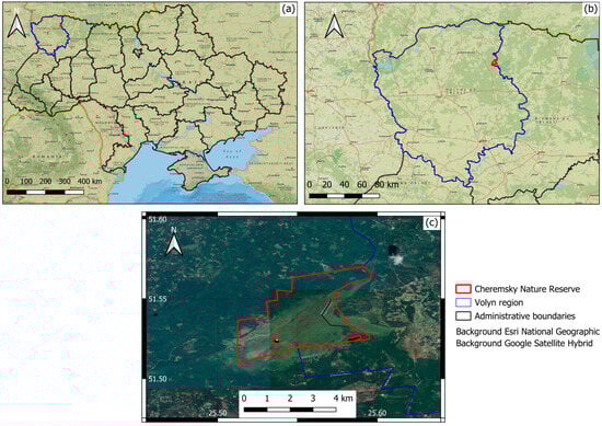
Figure 1.
(a) Location of the research object on the territory of Ukraine; (b) Location of the research object within the Volyn region; (c) Boundaries of the Cheremsky Nature Reserve.
The main goal of the Cheremsky Nature Reserve is to preserve the typical and unique natural complex of Western Polissya, which has important environmental, aesthetic, educational, historical, and cultural significance. In accordance with Article 16 of the Law of Ukraine On the Nature Reserve Fund, any economic activity and other activities that contradict the purpose of the reserve, disrupt the natural development of processes and phenomena, or pose a threat of harmful impact on its natural complexes or objects are prohibited on the territory of nature reserves, namely: construction of structures, roads not related to the activities of the reserves, making fires, arranging recreation areas, passage or driveway of unauthorized persons, or flying of aircraft and helicopters below 2000 m above the reserve. All types of forest management, harvesting of fodder and medicinal herbs, catching and killing of wild animals, hunting, fishing, and all types of excursions, except for walking tours, are prohibited. The reserve is remote from settlements, and there are no power lines or paved roads on its territory. The territory of the Cheremsky Nature Reserve is a fully protected area created for the purpose of preserving ecosystems in perpetuity.
The reserve is a natural-territorial complex where unbroken forests with a unique eumesotrophic (transitional, highly waterlogged) sedge–sphagnum bog Cheremske have been preserved, which is hardly disturbed by anthropogenic activity.
According to the physical and geographical zoning of the Volyn region, the territory of the Cheremsky Nature Reserve is the Novochervyshchansky district of the Verkhneprypiatsky sub-region of the Volyn Polissya oblast of the Polissya province of the mixed forest zone [23,24]. The physical and geographical features of the territory are determined by the geological structure, where the main role is played by chalk deposits, the peculiarity of anthropogenic deposits, the spread of glacial relief forms, and the presence of karst formations.
In geomorphological terms, the territory of the Cheremsky Nature Reserve belongs to the Volyn accumulative water-glacial plain with a fluvio-glacial gently undulating surface of the Dnipro glaciation. This is the Povorski-Manevychi end-morain geomorphological region of Volyn Polissya (on denudational Cretaceous and Paleogene basement). The peculiarity of the Cheremsky Nature Reserve’s geomorphological position is that its territory is located on the border of the Verkhneprypiatska lowland and the Volyn moraine ridge. This plain is composed of end-moraine deposits of the maximum stage of the Dnipro glaciation and is characterized by a peculiar hilly ridge relief [25].
The most common landforms are aeolian dunes and ramparts, glacial moraine hills, water-glacial landforms (kams, ozy), karst-suffusion sinkholes, water-glacial depressions, and depressions (lake hollows, marsh depressions, and cryogenic saucers). It should also be noted that the Cheremsky marsh complex, stretching from southwest to northeast with an eastern spur to the Veselukha River, is a relict fluvio-glacial foreland [25].
The Cheremsky bog is one of the largest and best-preserved bogs in Europe, which in 2016, was designated as a wetland of international importance under number 2272, as confirmed by the Ramsar Convention certificate [6]. It is especially important for the conservation of migratory birds that stop here for rest or nesting. The unique eumesotrophic sedge–sphagnum bog covers an area of almost 1300 hectares, with peat thickness of more than 10 m, and is a kind of freshwater storage reservoir with moderate runoff. It is the core of the Cheremsky Nature Reserve. In the post-glacial period (5–8 thousand years ago), the present Cheremsky marshland was a flowing lake, which eventually became overgrown, but 2 areas of open water mirror remained on its territory: Cheremske Lake (7.7 hectares), 7.6 m deep, and Redichi Lake (11 hectares), 4.5 m deep.
The study area is located within a zone of intensive water exchange and excessive moisture. The aquifer, situated at a shallow depth beneath the water table, exerts a significant influence on the occurrence of waterlogging. The hydrogeological structure is closely related to the Quaternary sediments and is determined by fluvioglacial, lake-bog, and marsh sediments.
The lithological and genetic complexes of water-resistant rocks have led to the division of groundwater into three distinct types [26]:
- groundwater of modern bog deposits;
- groundwater of upper Quaternary alluvial deposits;
- groundwater of middle Quaternary lake-alluvial deposits;
The first type of groundwater is pervasive, and its boundary coincides with the contour of the marshes. The rocks have been identified as peat, which is characterized by its water-resistant properties. The thickness of the aquifer ranges from 0.3 to 6 m. The aquifer is fed by atmospheric and groundwater sources. It is important to note that the areas of feeding and distribution do not coincide. The water level fluctuates with the seasons. During the summer months, when precipitation levels are at their lowest, the water level is recorded at depths of up to 0.5 m. Conversely, during the wet season, the water level rises to between 0.1 and 0.3 m above the daily surface.
The second type exhibits a general planar distribution. The aquifer is comprised of sands and partially sandy loams. The aquifer is estimated to be between 5 and 15 m thick and is underlain by alluvial formations of middle Quaternary lake-alluvial deposits, represented by sands, loams, and sandy loams. The absence of aged waterstops in the sole is indicative of the hydraulic connection of this horizon with the underlying one. The aquifer is sustained by atmospheric water, and the zones of feeding and distribution coincide. The water level exhibits seasonal fluctuations. In periods of reduced water levels, the water table is maintained at a depth of 0.5–1.5 m, while in elevated regions, it may exceed 1.5 m. During wet seasons, the water level approaches the daytime surface.
The third type of groundwater is distributed at a depth of approximately 28 m. Sands and sandy loams act as water-resistant rocks. Furthermore, loams have been identified as playing a significant role in local water resistance. The thickness of the water-resistant layer is 9–18 m. The water-resistant layer is sustained by infiltration from overlying horizons. The feeding area typically coincides with the spreading area. The absence of aged waterstops in the anthropogenic strata leads to the formation of a single aquifer complex of Quaternary sediments, as opposed to multiple aquifer complexes.
The hydrogeological features and geological structure of the area are instrumental in determining the nature and physical and geographical properties of the ecosystems, including the significant waterlogging of the territory, the humus-poor soils, and the diversity of ecotopes.
More than 760 species of vascular plants grow on the territory of the wetland [27], and 25% of all rare plants of Ukrainian Polissya are concentrated here. Fifty-seven species are listed in the Red Book of Ukraine. Thanks to the pod grass communities, the Cheremsky marsh was not drained, and in 1978, a nature reserve was created, and later, a nature reserve. Three species are included in the European Red List, namely: Ukrainian goat’s-eye (Tragopogon ucrainicus), Ukrainian hawthorn (Crataegus ucrainica), and Lithuanian smelter (Silene lithuanica). Five species are listed in Appendix I of the Bern Convention and fourteen in Appendix II of CITES.
2.2. Datasets
COPERNICUS/S2_SR_HARMONIZED is a dataset available through the Google Earth Engine that provides harmonized Sentinel-2 surface reflectance data [28]. The data comes from the Sentinel-2 satellites, which are part of the Copernicus program of the European Space Agency (ESA) [17]. Surface reflectance (SR) indicates that the data have been processed to remove atmospheric effects, providing more accurate measurements of the Earth’s surface reflectance. The dataset has been ‘harmonized’, meaning that data from different Sentinel-2 orbits have been brought to a consistent standard. This reduces the differences between images captured at different times or from different orbits, making it easier to analyze time series. The data are available at spatial resolutions of 10, 20, and 60 m, depending on the band. The dataset includes 13 Sentinel-2 spectral bands, from visible to short-wave infrared. In our work, we used median composite images (Table 1) for the period from 1 June to 31 August for 2017–2024.

Table 1.
Number of Sentinel 2 images used to create composites by year.
In this study, a temporal filter was applied to obtain imagery over a period of eight years (1 July–31 August for 2017–2024). Furthermore, a selection criterion was applied to identify images exhibiting less than 10% cloud contamination, given the deleterious effect that cloud-contaminated imagery has on analysis outcomes. The application of these criteria resulted in the availability of 533 images. The remaining cloudy pixels were masked out using a cloud-masking function, termed masksS2clouds, which relies on the QA60 band (i.e., the quality flag) used to identify clouds and cirrus. The final stage entailed the generation of a composite image devoid of cloud contamination by utilizing the median composite function within the Google Earth Engine (GEE). This process also enabled the elimination of pixels exhibiting extreme values, thus ensuring the removal of any residual artefacts. The resultant composite image was composed of pixels with minimal or no cloud cover.
2.3. Methodology
Based on the obtained composite images for the study area, random points were generated for the calculation and subsequent overlay of spectral indices for a certain time period.
2.3.1. Vegetation Indexes
The well-known and extensively utilized NDVI (normalized difference vegetation index) [29] is a straightforward yet powerful tool for measuring green vegetation. It balances the scattering of green leaves in near infra-red wavelengths with the absorption of chlorophyll in red wavelengths. NDVI values range from −1 to 1. Negative NDVI values (close to −1) indicate water. Values near zero (−0.1 to 0.1) usually represent barren areas, like rock, sand, or snow. Low, positive values (around 0.2 to 0.4) correspond to shrubs and grasslands, while high values denote temperate and tropical rainforests (Table 2).
Table 2.
Spectral indexes.
The enhanced vegetation index (EVI) [30] is a valuable tool for monitoring vegetation, especially in areas with dense canopy cover. The EVI is designed to enhance the vegetation signal by correcting for soil background signals and atmospheric influences. In areas of dense canopy cover, where the leaf area index (LAI) is high, the blue wavelengths can be used to improve the accuracy of NDVI, as it corrects for soil background signals and atmospheric influences. The range of values for EVI is −1 to 1, with healthy vegetation generally around 0.20–0.80 (Table 2).
The stability of NDVI products derived empirically has been demonstrated to be susceptible to variations in soil color, moisture, and saturation effects resulting from vegetation density. In an effort to enhance NDVI’s precision and reliability, article [31] described a novel soil-adjusted vegetation index that considers variations in red and near-infrared extinction through the vegetation canopy. This index is based on a transformation technique that aims at minimizing the influence of soil brightness from spectral vegetation indices involving red and near-infrared (NIR) wavelengths (Table 2).
The modified soil-adjusted vegetation index (MSAVI) has been devised [32] to serve as a substitute for the NDVI and NDRE when these indices are inadequate in supplying precise data due to factors such as insufficient vegetation or a paucity of chlorophyll in the plant tissue. During the germination and leaf development stages, a significant amount of bare soil is often present between seedlings. Conventionally, NDVI and NDRE have been interpreted as poor vegetative indicators in such contexts. In such instances, the MSAVI proves to be a valuable asset. “SA” in MSAVI denotes “soil-adjusted”, thereby highlighting the pivotal feature of this vegetation index. It has been demonstrated that MSAVI mitigates the impact of underlying soil characteristics on the calculation of vegetation density within the field context (Table 2).
GNDVI (green normalized difference vegetation index) has been defined [33] as an indicator of plant “greenness” or photosynthetic activity. It is a chlorophyll index that is employed at the later stages of development, as it saturates at a later point in time than NDVI. It is one of the most widely used vegetation indices in determining water and nitrogen uptake in the crop canopy. GNDVI exhibits heightened sensitivity to chlorophyll variation within the crop when compared with NDVI, and it attains a higher saturation point. It is particularly well-suited for applications in crops with dense canopies or in later stages of development, while NDVI is more suitable for estimating crop vigor in earlier stages (Table 2).
NDRE (normalized difference red-edge index) has been demonstrated [34] to be a superior indicator of vegetation health and vigor in comparison to NDVI for vegetation in the mid to late season stages that have accumulated high levels of chlorophyll in their leaves. This is attributable to the fact that red-edge light is more translucent to leaves than red light, and as a result, it is less likely to be completely absorbed by a canopy. Chlorophyll exhibits its maximal absorption in the red waveband; consequently, red light does not penetrate beyond a few leaf layers. Conversely, light in the green and red-edge regions can penetrate a leaf much more deeply than blue or red light. As a result, a pure red-edge waveband exhibits greater sensitivity to medium to high levels of chlorophyll content and, consequently, leaf nitrogen than a broad waveband that encompasses blue light, red light, or a mixture of visible and NIR light. This characteristic renders NDRE more suitable for intensive management applications throughout the growing season, as NDVI frequently exhibits a decline in sensitivity after plants attain a substantial level of leaf cover or chlorophyll content (Table 2).
In the context of monitoring vegetation in areas affected by drought, it is recommended to employ the NDWI (normalized difference water index) index proposed by Gao [35], which utilizes NIR and SWIR. The SWIR reflectance in this index is indicative of changes in both the vegetation water content and the spongy mesophyll structure in vegetation canopies. The NIR reflectance is influenced by the leaf internal structure and leaf dry matter content but not by water content. The integration of NIR and SWIR data effectively eliminates variations induced by the leaf internal structure and leaf dry matter content, thereby enhancing the accuracy of retrieving the vegetation water content [36]. This index has been employed in studies exploring water content at the single leaf level [36] as well as at the canopy/satellite level [37,38].
2.3.2. Correlation Analysis
Determining how different indices relate to each other helps to understand which ones can be interchangeable or complementary in analyzing vegetation cover, water balance, and other environmental parameters. Identification of strong correlations can help reduce the number of indices that need to be used in the analysis, which simplifies the data processing process and reduces computational costs. Correlation analysis helps to determine which indices have the greatest impact on changes in vegetation, water balance, or other environmental parameters, which is important for decision-making in agriculture, ecology, and natural resource management. Correlation analysis can detect anomalies or errors in the data, which allows for additional verification and validation of the collected information.
2.3.3. K-Means Point Classification
K-means classification is a popular clustering algorithm [39,40] in machine learning that belongs to unsupervised methods. It groups objects into k clusters based on the similarity of their characteristics. To determine the optimal number of clusters, it is proposed to calculate the average silhouette coefficient s(i) (1). The best value of s(i) is the one that maximizes the average silhouette coefficient.
where a(i)—the average distance from point i to all other points in the same cluster; b(i)—the average distance from point i to all points in the nearest neighboring cluster.
The elbow method (2) is a widely utilized approach for ascertaining the optimal number of clusters in clustering, particularly in the context of the K-means algorithm [41]. SSE (sum of squared errors) is a metric that quantifies the total distance between data points and their respective cluster centroids. SSE is calculated as the sum of the squared distances from each point to the nearest centroid. The underlying principle of this method is to identify the point on the SSE graph where the rate of decrease in SSE begins to exhibit a substantial decline. This point is referred to as the “elbow” on the graph. The optimal number of clusters is identified as the value of K at which the SSE graph exhibits a notable bend, indicating that the addition of new clusters does not result in a substantial decrease in SSE. The algorithm for minimizing the sum of squares of distances (within-cluster sum of squares, WCSS) is defined by:
where μi—the center of the Ci cluster.
2.3.4. Random Forest Feature Importance
Random forest [41] is a sophisticated machine learning algorithm that can be utilized for both classification and regression tasks. It integrates multiple decision trees to enhance the precision of predictions and manage noisy or incomplete data. A salient benefit of Random forest is its capacity to ascertain the relative importance of various features present within a dataset. The utilization of a bar chart is a viable method for the visualization of feature importance, thereby facilitating the acquisition of insights into the relative importance of each feature.
2.3.5. Principal Component Analysis (PCA)
Principal component analysis (PCA) is a data dimensionality reduction method [41] used to identify the main components that explain the largest part of the variation in the data. The procedure entails the transformation of the original variables into new variables, designated as principal components. These principal components are defined as linear combinations of the original variables, and they are also known as orthogonal components, meaning that they are uncorrelated with each other. The application of PCA enables the identification of the components that account for the maximum proportion of the observed variation in the data. The first component captures the maximum variation, the second component captures the second largest part, and so on. PCA facilitates the reduction of variables while preserving the majority of the information contained in the data.
Spectral indices, such as NDVI, EVI, SAVI, MSAVI, GNDVI, NDRE, and NDWI, exhibit significant intercorrelation. PCA facilitates the reduction of variables while preserving the essential information. The application of PCA facilitates the visualization of data in fewer dimensions, thereby enhancing the analysis and interpretation of the data. PCA facilitates the identification of the primary factors that influence the variation in the data. This ability to discern underlying mechanisms is crucial for understanding phenomena, such as vegetation health, water balance, and other environmental parameters.
The methodology used is described in the following flowchart (Figure 2).
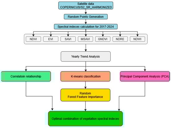
Figure 2.
Methodology flowchart.
3. Results
3.1. Trend Analysis and Correlation Relationship
The majority of the indices employed to evaluate the condition of vegetation (NDVI, SAVI, MSAVI, GNDVI, NDRE) demonstrate a negative trend during the period 2017–2024 (Figure 3). This suggests a probable decline in the overall condition of vegetation or the emergence of unfavorable changes within the designated area under analysis. The most significant declines are observed in NDVI and GNDVI, suggesting a potential decrease in green biomass or a decline in photosynthetic activity of vegetation. The potential causes of such negative trends encompass a wide range of factors, including but not limited to climate change (e.g., droughts, temperature changes), plant diseases, or other environmental stressors. Conversely, the EVI demonstrates virtually no trend. The EVI is designed to minimize atmospheric influence and signal saturation, and its stability may indicate that changes occurring in other indices or that the EVI is less sensitive to these changes in the context of the area and object of study may be more visible.
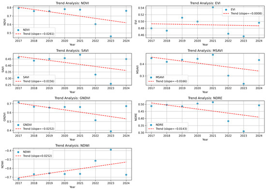
Figure 3.
Trend analysis of the median values of the NDVI, EVI, SAVI, MSAVI, GNDVI, NDRE, and NDWI indices for the period 2017–2024.
The indices NDVI, EVI, SAVI, MSAVI, GNDVI, and NDRE are typically used to reflect vegetation condition, photosynthetic activity, and chlorophyll concentration. A decrease in these indices may be indicative of a decline in biomass, plant stress, or alterations in cover composition. Excessive humidity and/or waterlogging have been identified as a potential contributing factor to such stress.
Conversely, the NDWI index, which is employed to evaluate water content, demonstrates a favorable trend. An increase in the NDWI may indicate an increase in the moisture content of the vegetation. Further research is required to determine the impact of climate on the NDWI using archived hydrometeorological data. It is imperative to ascertain whether this represents a genuine increase in water resources or a response to other alterations. Subsequent research endeavors are planned to address these inquiries.
Based on the obtained spectral indices for the period from 2017 to 2024, we have obtained the following relation (Figure 4). The matrix of correlation relationships for the entire period of observation is presented in Table 3.
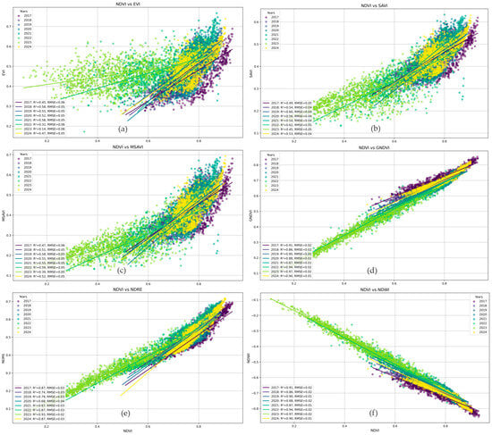
Figure 4.
Relations for 2017–2024 between NDVI and: (a) EVI; (b) SAVI; (c) MSAVI; (d) GNDVI; (e) NDRE; and (f) NDWI.
Table 3.
The correlation matrix between the spectral indexes for the years 2017–2024.
The correlation analysis shows high positive correlations between NDVI and GNDVI (0.98), as both indices are based on normalized difference, but GNDVI uses green and NIR bands, while NDVI uses red and NIR bands. A high correlation indicates that these indices are interchangeable and reflect very similar vegetation characteristics.
The high positive correlation between NDVI and NDRE (0.93) indicates that NDRE is sensitive to the chlorophyll content, especially in dense vegetation. The high correlation with NDVI shows that both indices reflect the overall condition of the vegetation, although NDRE is more sensitive to variations in chlorophyll. There is a high positive correlation between NDVI and SAVI (0.86) and MSAVI (0.83), which are indices that try to minimize the influence of soil background on vegetation measurements. The high correlation with NDVI shows that even when corrected for soil, they are still highly correlated with the overall NDVI vegetation index. The very high positive correlation with SAVI and MSAVI (0.99) is not surprising, as both indices are “soil-corrected” versions of NDVI, and therefore, their behavior is almost identical. The high positive correlation of GNDVI and NDRE (0.91) confirms their similar sensitivity to vegetation condition, although GNDVI is more general and NDRE is more sensitive to chlorophyll.
The high negative correlation between NDVI and NDWI (−0.98) is due to the fact that NDWI is an index that reflects the water content of vegetation. The negative correlation with NDVI is logical: greener vegetation (high NDVI) is usually associated with less water stress (and possibly higher water content), although this is a simplistic assumption and the relationship is complex. The perfect negative correlation of GNDVI and NDWI (−1.00) is very unusual and suspicious. It may indicate a very specific situation where these two indices are perfectly inversely related. This requires further verification and research. The high negative correlation of NDRE and NDWI (−0.91), similar to NDVI and NDWI, confirms the inverse relationship between vegetation condition and water index. The high negative correlation of SAVI and NDWI (−0.84) and MSAVI and NDWI (−0.80), similar to NDVI and NDWI, given that SAVI and MSAVI are already corrected for soil, the correlation still remains strongly negative with the water index.
The moderate correlation of EVI with NDVI (0.47), SAVI (0.72), MSAVI (0.77), GNDVI (0.39), and NDRE (0.44) can be explained by the fact that EVI (enhanced vegetation index) is designed to reduce the influence of atmosphere and soil, as well as to improve sensitivity to high biomass, where NDVI can “saturate”. The moderate correlation with the other indices, especially NDVI and GNDVI, may indicate that EVI does capture more detailed information more related to canopy structure and/or leaf area index (LAI) than just overall “greenness” and may be more sensitive to the specific conditions in this dataset.
3.2. K-Means Clustering and Feature Importance
Prior to initiating the K-Means clustering process, the number of classes was estimated through the application of the elbow method and the silhouette analysis (Table 4). The outcomes of this analysis yielded an SSE of 169.834 and a silhouette score of 0.408, indicating that the optimal number of clusters (K) is three (Figure 5).
Table 4.
Results of determining the optimal number of clusters.
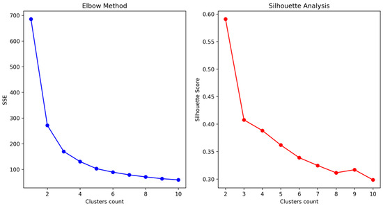
Figure 5.
Results of application of the elbow method and the silhouette analysis.
The distribution of points according to the classification class is shown in Figure 6. The distribution of the number of points by classification classes by year is shown in Figure 7.
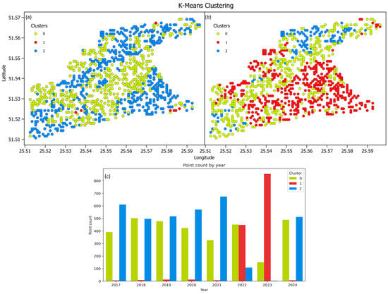
Figure 6.
Results of K-Means clustering using K = 3, (a) using median values of indexes for 2017–2024, (b) using values for 2022, and (c) annual distribution of points by clusters.
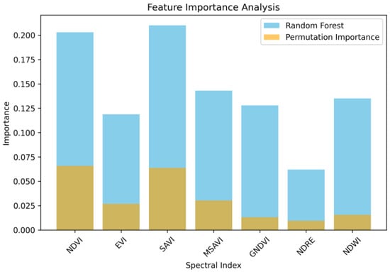
Figure 7.
Random forest feature importance analysis and permutation importance.
Visual interpretation allows us to establish that in 2022–2023 the number of points corresponding to class 1-open water, was significantly higher compared to the median values for all years. This can explain the significant increase in the values of the NDVI index and the decrease in the rest of the indices.
The evaluation of the accuracy of feature importance in a random forest model using permutation importance is a critical step in ascertaining the reliability of the feature ranking results. Permutation importance has been demonstrated to be a potent and accessible approach to assessing the impact of individual features on the model’s precision.
The random forest model, an ensemble of decision trees, inherently provides an estimate of the importance of the features utilized in constructing the trees. This “built-in” feature importance, frequently referred to as mean decrease impurity or Gini importance for classification and mean decrease accuracy for regression, is calculated based on the extent to which each feature reduces impurity or enhances accuracy at each branch in the forest.
Permutation importance, also known as “mean decrease accuracy” in the context of random forest, is an alternative method of evaluating feature importance that tries to circumvent some of the limitations of embedded importance [42,43]. This method involves training a random forest model on the entire dataset, subsequently measuring the baseline accuracy, thereby establishing a reference accuracy. Subsequently, for each feature, the values in the validation or test dataset are shuffled. Concurrently, the values of all other features remain constant. This process, known as “shuffling,” disrupts the original relationship between a specific feature and the target variable while preserving the distribution of feature values. The key idea is that if a particular feature is important for making accurate predictions, disrupting its values should significantly degrade the model’s performance when compared to the baseline. Conversely, if shuffling a feature does not change the accuracy much, then that feature likely contributed little to the predictions.
Subsequent to this process, the accuracy of the trained model on this modified dataset is re-evaluated. The permutation importance of a feature (PI) is calculated as the difference between the baseline accuracy (BA) and the accuracy after shuffling (SA) (3).
The results of the random forest feature importance analysis and permutation importance can be observed in Figure 7.
The analysis of the results clearly shows that the NDVI and SAVI adjusted for soil influence are the most significant in our study.
Principal Component Analysis (PCA)
The impact of spectral indices on principal components (PCA) was analyzed for the entire set of spectral index values obtained for the period 2017–2024. The ensuing findings are presented in graphical form in Figure 8.
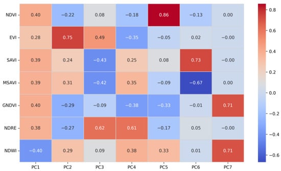
Figure 8.
Impact of spectral indices on principal components (PCA).
The results of the principal component analysis (PCA) demonstrate the structure of the principal components of variation in the set of vegetation indices under consideration. Through the analysis of component loadings, we can discern the indices that exert the most significant influence on each principal component (PC) and elucidate the potential representation of these components.
It is evident that PC1 primarily exemplifies the primary axis of variability, thereby delineating the extent of the vegetation’s overall “greenness” (vegetation indices) in relation to its moisture content (NDWI). High PC1 values can indicate areas with dense vegetation and low water content, or vice versa. This may be the predominant gradient characterizing the bogs under study, particularly reflecting a gradient from dry to wetter areas or from dense to sparse vegetation.
PC2 demonstrates a notable correlation with EVI, suggesting its potential to differentiate EVI from other general vegetation indices. The positive loadings for MSAVI, SAVI, and NDWI may suggest that PC2 also reflects certain aspects that EVI shares with these indices, potentially related to canopy structure or water response, distinct from the underlying “greenness” characterized by NDVI and GNDVI. The contrasting nature of the loadings for NDVI, GNDVI, and NDRE, which are negative, in relation to the predominantly positive EVI, underscores the distinct information provided by these indices.
The third principal component, PC3, is predominantly influenced by NDRE, with a modest contribution from EVI. The negative loadings observed for SAVI and MSAVI suggest that PC3 may reflect an aspect that is more effectively captured by NDRE and EVI compared to the soil-adjusted indices. This phenomenon may be attributed to vegetation characteristics, such as chlorophyll content or structural features, which NDRE is more sensitive to.
PC4 demonstrates a notable correlation with NDRE, exhibiting a positive association with NDWI and soil-adjusted indices (MSAVI, SAVI) and a negative correlation with EVI. This observation may signify an aspect pertaining to the interaction between water content and the structural characteristics of vegetation that NDRE is capable of extracting.
PC5 is predominantly influenced by NDVI, exhibiting a positive correlation with NDWI and a negative correlation with GNDVI. The separation of NDVI and GNDVI in PC5 is particularly noteworthy, given the strong correlation between these variables in the original correlation matrix. This observation may signify the presence of subtle variations in variability that become evident in the reduced PCA dimensional space.
PC6 exhibits a pronounced distinction between SAVI and MSAVI. Given the soil adjustment of both indices and their high correlation, this component likely reflects subtle differences in the methods by which these indices correct for soil effects and their specific sensitivity to varying soil or vegetation conditions.
The PC7 index is predominantly influenced by two indices: GNDVI and NDWI. Furthermore, the loadings for GNDVI and NDWI are almost identical in absolute value and sign (both positive and around 0.707). The contributions of all other indices to PC7 are negligible, as evidenced by their insignificant loadings.
4. Discussion
The present study set out to analyze the spatial and temporal changes in spectral indices in order to assess the state of marshes. The study was conducted on the example of the Cheremskyi Nature Reserve in Volyn Region. The analysis revealed several important patterns. For the period from 2017 to 2024, the majority of indices reflecting vegetation status (NDVI, SAVI, MSAVI, GNDVI, NDRE) exhibited negative trends, suggesting a potential deterioration in the ecosystem’s overall condition, particularly a decline in greenness, photosynthetic activity, and plant biomass. Conversely, the positive trend of NDWI signifies an augmentation in water content, which may be attributable to both an increase in humidity in the bogs and alterations in the composition of the vegetation cover. This observation aligns with the results reported in other studies, which also documented changes in spectral characteristics during the monitoring of marshes across various regions [12,19,21].
An analysis of the vegetation trend graphs reveals a general tendency towards the deterioration of vegetation conditions, as indicated by a decline in NDVI, SAVI, MSAVI, GNDVI, and NDRE, and an increase in potential water content, as indicated by a rise in NDWI, in the designated area from 2017 to 2024. The correlation analysis demonstrated a high degree of positive correlation between NDVI, GNDVI, SAVI, MSAVI, and NDRE, indicating their shared capacity to serve as indicators of the plant condition, despite variations in the utilization of distinct spectral bands. For instance, the high correlation coefficient between NDVI and GNDVI (≈0.98) confirms their interchangeability, while the inverse correlation with NDWI (down to −0.98) indicates the specificity of measuring water balance with these indices. The outcomes of this study are consistent with those reported by Taddeo et al. [21] and Li et al. [19], who attributed analogous relationships to the impact of hydrological conditions on the dynamics of vegetation cover in marsh ecosystems. In this context, it is especially worth paying attention to the latest specialized water indices for the multispectral systems Landsat-8, 9 and Sentinel-2, such as SMBWI (Sentinel multi-band water index) [44] and WIW (water in wetlands) [45] with overall accuracy of water maps > 96.5% and up to 94%, respectively. The positive trend in NDWI suggests an increase in vegetation water content, which may be indicative of improved water availability or changes in vegetation types. However, the high negative correlation between NDWI and other vegetation indices (NDVI, GNDVI, NDRE) underscores the complex relationship between vegetation health and water content. This necessitates further investigation to disentangle the effects of water stress and other environmental factors on vegetation dynamics.
The application of clustering methods (K-Means) and the analysis of the importance of features using random forest (using permutation importance) allowed the researchers to reveal the heterogeneity of bogs in terms of vegetation and water regime. The identification of three distinct clusters lends further credence to the notion that bogs can be categorized into multiple types, each exhibiting distinctive spectral characteristics. This finding is consistent with the conclusions of analogous classical studies [39,40]. A comparison of the data obtained with other works on the classification and monitoring of bogs (e.g., Kumar and Singh [41]) confirms the feasibility of using integrated approaches that combine the analysis of spectral indices with modern machine learning methods.
Principal component analysis (PCA) was utilized to identify the primary axes of variation in the dataset under investigation. PC1, which favorably reflects the contrast between vegetation greenness (NDVI, GNDVI) and water balance (NDWI), is a key axis characteristic of bogs, where hydrology and plant condition have a significant impact on ecological function. This approach has been previously employed in other studies to identify the primary factors influencing the variability of bogs [21,24].
EVI and NDRE are accentuated in PC2, PC3, and PC4, signifying that they offer distinctive information that differs from general indices such as NDVI and GNDVI. When seeking to discern more nuanced aspects of vegetation health, canopy structure, or chlorophyll content, it is recommended to consider EVI and NDRE.
While NDVI and GNDVI exhibit strong correlations, they demonstrate independent variability in the higher PCs, particularly PC5. In many instances, utilizing a single index, typically NDVI due to its familiarity, might suffice. However, in scenarios where maximum sensitivity is paramount, employing both indices or basing decisions on their respective PC loadings might be justified.
The disparities between SAVI and MSAVI in PC6 suggest that, despite their shared classification as soil-adjusted indices, they may exhibit sensitivity to varying soil types or levels of vegetation cover. Consequently, for studies centered on soil impacts, the analysis of the disparities between SAVI and MSAVI as presented by PC6 may prove beneficial.
The NDWI, on the other hand, exhibits distinct behavior (often contrary to vegetation indices), which is rational given its measurement of a distinct environmental variable, water content.
5. Recommendations
In order to achieve a comprehensive wetland monitoring, it is recommended to prioritize the following vegetation indices:
- Both indices NDVI or GNDVI are strongly represented in PC1 and reflect the overall vegetation condition (”greenness“). Given their high correlation, the selection of one index over the other can be made to reduce redundancy. While NDVI is more conventional and extensively utilized, GNDVI might be preferable if sensitivity to the green spectrum is a salient factor.
- NDWI is paramount for monitoring the water content and is distinctly emphasized in PC1 and PC7. Its inclusion is imperative in the assessment of the hydrological condition of bogs.
- EVI is presented in PC2 and PC3, providing additional information on vegetation canopy structure and biomass. It is less sensitive to atmospheric and soil effects than NDVI. The incorporation of EVI can enhance our comprehension of the structural characteristics of wetland vegetation.
- NDRE exerts a substantial influence on PC3 and PC4, underscoring its significance in evaluating chlorophyll content and vegetation health, particularly in dense stands. The utilization of NDRE can facilitate the discernment of alterations in the physiological state of wetland vegetation.
A particularly promising area of research is the combination of synthetic aperture radar (SAR, e.g., Sentinel-1) data with Sentinel-2 optical imagery. This approach will provide additional information on surface moisture, vegetation structure, and flooding, which will help improve the quality of classification and forecasting of changes in marsh ecosystems [14,20].
The further implementation of deep learning algorithms for processing multispectral and radar data can achieve higher accuracy in recognizing different types of marshes, as well as identify complex nonlinear relationships between environmental indicators. Long-term monitoring, incorporating considerations of both climate and anthropogenic impacts, is imperative.
It is recommended that the time range of the analysis be extended and that additional parameters, including temperature, precipitation, and solar radiation intensity, be incorporated to enhance comprehension of the impact of climate change on the state of the wetlands. The utilization of field measurements to verify satellite data will enhance the reliability of the results.
The creation of composite indices or multi-index models that take into account the interaction of different spectral parameters will allow for a more comprehensive characterization of ecosystem processes in wetlands and the development of effective early warning tools for degradation.
In summary, the findings of this study underscore the necessity for a comprehensive multi-index approach to the monitoring of wetlands and highlight the importance of further research aimed at integrating heterogeneous data and applying modern analytical methods to understand the processes occurring in these fragile ecosystems [1,12,19,20,21]. The implementation of these measures will facilitate the development of more effective strategies for the conservation and sustainable utilization of wetland biodiversity, a critical consideration in the context of global climate change and increasing anthropogenic pressure.
Author Contributions
Conceptualization, O.M.; methodology, O.M.; software, O.M.; validation, O.M.; formal analysis, O.M.; investigation, O.M.; resources, O.M.; data curation, O.M.; writing—original draft preparation, O.M. and A.B.; writing—review and editing, O.M. and A.B.; visualization, O.M.; supervision, A.B.; project administration, A.B.; funding acquisition, A.B. All authors have read and agreed to the published version of the manuscript.
Funding
This research was funded by Deutscher Akademischer Austauschdienst in program Future Ukraine: Research Grants for Ukrainian Master’s students and researchers, 2024/2025 (57755101). APC was funded by the Technical University of Applied Sciences Würzburg-Schweinfurt, 97070 Würzburg, Germany.
Data Availability Statement
The data used to support the findings of this study are available from the corresponding author upon request.
Acknowledgments
The author thanks the reviewers for reading and reviewing this manuscript.
Conflicts of Interest
The authors declare no conflicts of interest.
References
- Kulish, I.; Kaplenko, H.; Martyniuk, U.; Semchuk, I.; Kravtsiv, I.; Dorosh, M.; Chemerys, V. Harnessing the Resource Potential of Wetlands:The Environmental Context. Ukr. J. Ecol. 2021, 11, 117–123. [Google Scholar]
- Frolking, S.; Talbot, J.; Jones, M.C.; Treat, C.C.; Kauffman, J.B.; Tuittila, E.S.; Roulet, N. Peatlands in the Earth’s 21st Century Climate System. Environ. Rev. 2011, 19, 371–396. [Google Scholar] [CrossRef]
- Harenda, K.M.; Lamentowicz, M.; Samson, M.; Chojnicki, B.H. The Role of Peatlands and Their Carbon Storage Function in the Context of Climate Change. In Interdisciplinary Approaches for Sustainable Development Goals; GeoPlanet: Earth and Planetary Sciences; Springer: Cham, Switzerland, 2018; pp. 169–187. [Google Scholar] [CrossRef]
- Convention on Wetlands. Global Guidelines for Peatland Rewetting and Restoration; Secretariat of the Convention on Wetlands: Gland, Switzerland, 2021. [Google Scholar]
- Ukraine Needs Peatland Management Reform: Appeal to the Government and the Ministry of Environmental Protection|WWF. Available online: https://www.wwf.mg/en/?16768916/Ukraina-potrebuye-reformy-povodzhennya-torfovyshchamy-zvernennya-do-Uriadu-ta-Ministerstva-zakhystu-dovkillya (accessed on 13 March 2025).
- Cheremske Bog|Ramsar Sites Information Service. Available online: https://rsis.ramsar.org/ris/2272 (accessed on 10 March 2025).
- Solovey, T. Wetlands of the Volhynian Polissia (Western Ukraine): Classification, Natural Conditions of Distribution and Spatial Difference. Geol. Q. 2019, 63, 139–149. [Google Scholar] [CrossRef]
- Konishchuk, V.V.; Skakalska, O.I. Drosera in Ukraine: Ecological, Сhorological Specifics and Phytosozonomical Characteristics. Biosyst. Divers. 2019, 27, 3–15. [Google Scholar] [CrossRef]
- Martyniuk, V.; Korbutiak, V.; Hopchak, I.; Pryshchepa, A.; Zubkovych, I.; Shuliakovska, A. Landscape and Limnology Monitoring of Reservoirs in Cheremskyi Nature Reserve. In Proceedings of the 16th International Conference Monitoring of Geological Processes and Ecological Condition of the Environment, Kyiv, Ukraine, 15–18 November 2022; Volume 2022, pp. 1–6. [Google Scholar] [CrossRef]
- Danylyk, I.; Sosnovska, S.; Kuzyarin, O.; Kuzmishyna, I.; Kotsun, L. Monitoring of Rare Vascular Plant Populations in Cheremskyi Nature Reserve (Volyn Region, Ukraine). Notes Curr. Biol. 2018, 8, 40–48. [Google Scholar] [CrossRef]
- Trofymenko, P.; Zatserkovnyi, V.; Kartak, V.; Trofimenko, N.; Karas, I.; Borysov, F. Development of GIS for Assessment of Soil Potential of Polissya of Ukraine. In Proceedings of the International Conference of Young Professionals «GeoTerrace-2020», Lviv, Ukraine, 7–9 December 2020; Volume 2020, pp. 1–5. [Google Scholar] [CrossRef]
- Zhang, S.; Na, X.; Kong, B.; Wang, Z.; Jiang, H.; Yu, H.; Zhao, Z.; Li, X.; Liu, C.; Dale, P. Identifying Wetland Change in China’s Sanjiang Plain Using Remote Sensing. Wetlands 2009, 29, 302–313. [Google Scholar] [CrossRef]
- Frohn, R.C.; Reif, M.; Lane, C.; Autrey, B. Satellite Remote Sensing of Isolated Wetlands Using Object-Oriented Classification of Landsat-7 Data. Wetlands 2009, 29, 931–941. [Google Scholar] [CrossRef]
- Ozesmi, S.L.; Bauer, M.E. Satellite Remote Sensing of Wetlands. Wetl. Ecol. Manag. 2002, 10, 381–402. [Google Scholar] [CrossRef]
- Kaplan, G.; Avdan, U. Monthly Analysis of Wetlands Dynamics Using Remote Sensing Data. ISPRS Int. J. Geo-Inf. 2018, 7, 411. [Google Scholar] [CrossRef]
- Sun, T.; Lin, W.; Chen, G.; Guo, P.; Zeng, Y. Wetland Ecosystem Health Assessment through Integrating Remote Sensing and Inventory Data with an Assessment Model for the Hangzhou Bay, China. Sci. Total Environ. 2016, 566–567, 627–640. [Google Scholar] [CrossRef]
- Sentinel-2-Sentinel Online. Available online: https://sentinels.copernicus.eu/copernicus/sentinel-2 (accessed on 13 March 2025).
- Gorelick, N.; Hancher, M.; Dixon, M.; Ilyushchenko, S.; Thau, D.; Moore, R. Google Earth Engine: Planetary-Scale Geospatial Analysis for Everyone. Remote Sens. Environ. 2017, 202, 18–27. [Google Scholar] [CrossRef]
- Li, L.; Vrieling, A.; Skidmore, A.; Wang, T.; Muñoz, A.R.; Turak, E. Evaluation of MODIS Spectral Indices for Monitoring Hydrological Dynamics of a Small, Seasonally-Flooded Wetland in Southern Spain. Wetlands 2015, 35, 851–864. [Google Scholar] [CrossRef]
- Amani, M.; Salehi, B.; Mahdavi, S.; Brisco, B. Spectral Analysis of Wetlands Using Multi-Source Optical Satellite Imagery. ISPRS J. Photogramm. Remote Sens. 2018, 144, 119–136. [Google Scholar] [CrossRef]
- Taddeo, S.; Dronova, I.; Depsky, N. Spectral Vegetation Indices of Wetland Greenness: Responses to Vegetation Structure, Composition, and Spatial Distribution. Remote Sens. Environ. 2019, 234, 111467. [Google Scholar] [CrossRef]
- УКАЗ ПРЕЗИДЕНТА УКРАЇНИ №1234/2001—Офіційне Інтернет-Представництвo Президента України. Available online: https://www.president.gov.ua/documents/12342001-213 (accessed on 13 March 2025).
- Martyniuk, V.; Korbutiak, V.; Hopchak, I.; Kovalchuk, I.; Zubkovych, I. Methodology for Assessing the Geoecological State of Landscape-Lake Systems and Their Cartographic Modelling (Case Study of Lake Bile, Rivne Nature Reserve, Ukraine). Baltica 2023, 36, 13–29. [Google Scholar] [CrossRef]
- Kovalchuk, I.P.; Martyniuk, V.A. Methodology and Experience of Landscape-Limnological Research into Lake-Basin Systems of Ukraine. Geogr. Nat. Resour. 2015, 36, 305–312. [Google Scholar] [CrossRef]
- Pavlovska, T.S.; Kovalchuk, I.P. Geomorphology: Textbook for Students of Higher Education Institutions; VezhaDruk: Lutsk, Ukraine, 2022. [Google Scholar]
- Onishchuk, V.V. Estimation of Difersity Ecosystems Cheremskyi Natural Reserve on the Basis of Cartographical Modelling. Ph.D. Thesis, Kyiv National Taras Shevchenko University, Kyiv, Ukraine, 2006. [Google Scholar]
- Boyarin, M.V.; Savchuk, L.A. Ecological Description of Rare Species of Plants of Cheremskyi Nature Reserve Included in International Red Lists. Man Environ. Issues Neoecol. 2017, 1–2, 77–85. [Google Scholar] [CrossRef]
- Harmonized Sentinel-2 MSI: MultiSpectral Instrument, Level-2A (SR)|Earth Engine Data Catalog|Google for Developers. Available online: https://developers.google.com/earth-engine/datasets/catalog/COPERNICUS_S2_SR_HARMONIZED#terms-of-use (accessed on 13 March 2025).
- Crippen, R.E. Calculating the Vegetation Index Faster. Remote Sens. Environ. 1990, 34, 71–73. [Google Scholar] [CrossRef]
- Huete, A.; Didan, K.; Miura, T.; Rodriguez, E.P.; Gao, X.; Ferreira, L.G. Overview of the Radiometric and Biophysical Performance of the MODIS Vegetation Indices. Remote Sens. Environ. 2002, 83, 195–213. [Google Scholar] [CrossRef]
- Huete, A.R. A Soil-Adjusted Vegetation Index (SAVI). Remote Sens. Environ. 1988, 25, 295–309. [Google Scholar] [CrossRef]
- Qi, J.; Chehbouni, A.; Huete, A.R.; Kerr, Y.H.; Sorooshian, S. A Modified Soil Adjusted Vegetation Index. Remote Sens. Environ. 1994, 48, 119–126. [Google Scholar] [CrossRef]
- Barnes, E.; Clarke, T.R.; Richards, S.E.; Colaizzi, P.; Haberland, J.; Kostrzewski, M.; Waller, P.; Choi, C.; Riley, E.; Thompson, T.L. Coincident Detection of Crop Water Stress, Nitrogen Status, and Canopy Density Using Ground Based Multispectral Data. In Proceedings of the Fifth International Conference on Precision Agriculture, Bloomington, MN, USA, 16–19 July 2000. [Google Scholar]
- Gitelson, A.; Merzlyak, M.N. Quantitative Estimation of Chlorophyll-a Using Reflectance Spectra: Experiments with Autumn Chestnut and Maple Leaves. J. Photochem. Photobiol. B Biol. 1994, 22, 247–252. [Google Scholar] [CrossRef]
- Gao, B.C. NDWI—A Normalized Difference Water Index for Remote Sensing of Vegetation Liquid Water from Space. Remote Sens. Environ. 1996, 58, 257–266. [Google Scholar] [CrossRef]
- Ceccato, P.; Flasse, S.; Tarantola, S.; Jacquemoud, S.; Grégoire, J.M. Detecting Vegetation Leaf Water Content Using Reflectance in the Optical Domain. Remote Sens. Environ. 2001, 77, 22–33. [Google Scholar] [CrossRef]
- Serrano, J.; Shahidian, S.; da Silva, J.M. Evaluation of Normalized Difference Water Index as a Tool for Monitoring Pasture Seasonal and Inter-Annual Variability in a Mediterranean Agro-Silvo-Pastoral System. Water 2019, 11, 62. [Google Scholar] [CrossRef]
- Dennison, P.E.; Roberts, D.A.; Peterson, S.H.; Rechel, J. Use of Normalized Difference Water Index for Monitoring Live Fuel Moisture. Int. J. Remote Sens. 2005, 26, 1035–1042. [Google Scholar] [CrossRef]
- McCool, M.; Robison, A.D.; Reinders, J. K-Means Clustering. In Structured Parallel Programming; Elsevier: Amsterdam, The Netherlands, 2012. [Google Scholar]
- Melnyk, O.; Manko, P.; Brunn, A. Remote Sensing Methods for Estimating Tree Species of Forests in the Volyn Region, Ukraine. Front. For. Glob. Change 2023, 6, 5. [Google Scholar] [CrossRef]
- Umargono, E.; Suseno, J.E.; Vincensius Gunawan, S. K-Means Clustering Optimization Using the Elbow Method and Early Centroid Determination Based on Mean and Median Formula. In Proceedings of the 2nd International Seminar on Science and Technology (ISSTEC 2019), Yogyakarta, Indonesia, 25–26 November 2019. [Google Scholar] [CrossRef]
- Altmann, A.; Toloşi, L.; Sander, O.; Lengauer, T. Permutation Importance: A Corrected Feature Importance Measure. Bioinformatics 2010, 26, 1340–1347. [Google Scholar] [CrossRef]
- Loh, W.Y. Classification and Regression Trees. Wiley Interdiscip. Rev. Data Min. Knowl. Discov. 2011, 1, 14–23. [Google Scholar] [CrossRef]
- Su, Z.; Xiang, L.; Steffen, H.; Jia, L.; Deng, F.; Wang, W.; Hu, K.; Guo, J.; Nong, A.; Cui, H.; et al. A New and Robust Index for Water Body Extraction from Sentinel-2 Imagery. Remote Sens. 2024, 16, 2749. [Google Scholar] [CrossRef]
- Lefebvre, G.; Davranche, A.; Willm, L.; Campagna, J.; Redmond, L.; Merle, C.; Guelmami, A.; Poulin, B. Introducing WIW for Detecting the Presence of Water in Wetlands with Landsat and Sentinel Satellites. Remote Sens. 2019, 11, 2210. [Google Scholar] [CrossRef]
Disclaimer/Publisher’s Note: The statements, opinions and data contained in all publications are solely those of the individual author(s) and contributor(s) and not of MDPI and/or the editor(s). MDPI and/or the editor(s) disclaim responsibility for any injury to people or property resulting from any ideas, methods, instructions or products referred to in the content. |
© 2025 by the authors. Licensee MDPI, Basel, Switzerland. This article is an open access article distributed under the terms and conditions of the Creative Commons Attribution (CC BY) license (https://creativecommons.org/licenses/by/4.0/).