Quantum Tensor DBMS and Quantum Gantt Charts: Towards Exponentially Faster Earth Data Engineering

Abstract

Earth data is essential for global environmental studies. Many Earth data types are naturally modeled by multidimensional arrays (tensors). Array (Tensor) DBMSs strive to be the best systems for tensor-related workloads and can be especially helpful for Earth data engineering, which takes up to 80% of Earth data science. We present a new quantum Array (Tensor) DBMS data model and new quantum approaches that rely on the upcoming quantum memory and demonstrate exponential speedups when applied to many of the toughest Array (Tensor) DBMS challenges stipulated by classical computing and real-world Earth data use-cases. We also propose new types of charts: Quantum Gantt (QGantt) Charts and Quantum Network Diagrams (QND). QGantt charts clearly illustrate how multiple operations occur simultaneously across different data items and what are the input/output data dependencies between these operations. Unlike traditional Gantt charts, which typically track project timelines and resources, QGantt charts integrate specific data items and operations over time. A Quantum Network Diagram combines several QGantt charts to show dependencies between multistage operations, including their inputs/outputs. By using a static format, QGantt charts and Quantum Network Diagrams allow users to explore complex processes at their own pace, which can be beneficial for educational and R&D purposes.

1. Introduction

Earth data is essential for understanding global environmental changes. However, researchers and practitioners typically spend up to 80% of their time on data engineering, including data collection, organization, management, cleaning, transformation, and other issues to make data usable for subsequent modeling, analysis, ML/AI, and other purposes [1,2]. In addition, Earth data science faces ever increasing Earth data volumes. For example, ECMWF (European Centre for Medium-Range Weather Forecasts) stores 510 PB and ingests 287 TB/day [3] while about 203 TiB of products from Sentinels, a family of European satellite missions, are disseminated daily with total downloads of $80.5$ PiB/year [4]. Therefore, the scalability and performance of Earth data engineering tools are essential for enabling faster hypothesis testing and valuable insight discovery.

An important observation is that a multidimensional array (tensor) is a natural representation for a wide variety of Earth data types: diverse grids, meshes, swaths, and other constructs [5,6]. At the same time, a multidimensional array (tensor) is a native data model of Array (Tensor) DBMSs (Data Base Management Systems) [7,8,9] and a natural choice for fundamental datasets in countless domains: physics [7,10,11], geo-, bio-informatics [12,13,14,15], climate science [5,6,16,17], medicine [18,19,20], astronomy [21,22,23,24], e-commerce [25,26,27], and machine learning [28,29,30,31], to name a few.

Big Earth Data is one of the traditional and well-developed areas of Array (Tensor) DBMS applications [17,32,33,34], inspiring and attracting large multi-disciplinary teams building Cloud solutions and Earth Data Cubes using Array (Tensor) DBMSs  [35,36,37]. Array (Tensor) DBMSs have “natural affinity for remote sensing and geospatial data” [33], which are crucial for global ecological studies. Array (Tensor) DBMSs operate on personal computers, in the Cloud [32], and are even placed into satellite platforms for on-board processing of Big Earth Data [38]. Array (Tensor) DBMSs are also utilized in Precision Agriculture (e.g., detect pests, manage vegetation cycles, predict crop yield) [39,40,41], Forest Monitoring [42,43], Urban Planning [44,45], Water Management [46,47], Air Quality Control [48,49], and other environmental applications based on Big Earth Data [50,51,52,53].

Array (Tensor) DBMSs are relatively young systems that are gaining increasing attention and aim to be the best for tensor-oriented workloads related to storage [7,12,54,55,56], dissemination [9,57], management [58,59,60], processing [61], visualization [62,63,64], and even physical world simulations [65,66]. Array (Tensor) DBMSs address the challenges of big array storage, dissemination, management, processing, visualization, and diverse simulations [7,12,57,61,66]. We elaborate on the naming of Array (Tensor) DBMSs in Section 4.2.

Big array data is a primary source driving recent energy and excitement in array-oriented R&D: ChronosDB [17,57], SciDB [67], TileDB [56], ArrayStore [24], Google Earth Engine [68,69], SAGA  [70], EarthServer  [71], DataCube  [34], GeoTrellis  [72], Dask  [73], Microsoft Planetary Computer  [74], and other array systems appeared within just around a decade [13,17,28]. Impressive array-focused efforts are not surprising. For example, Google Earth Engine alone provides over 90 PB of data [75].

Efficient big array data management is challenging, so array R&D is blossoming with specialized, array-tailored techniques. Considerable effort was devoted to array storage layouts and compression schemes to improve I/O and compute time [9,14,54,56,67,76,77]. Arrays are also often stored out-db, so the problem is complicated by the need to optimize in-situ queries that use arrays in their native formats [17,70,78,79,80,81]. Indexing techniques, array joins, and tunable queries also pose challenging problems that can result in long runtimes [12,59,82]. Similarly, important array operations, including top-k queries, view maintenance, and caching use optimization heuristics [58,60,83]. Demanding applications like fast interactive visualization [57,63,64] and machine learning [28,29,30] directly impact user experience if not optimized quickly and properly. Array (Tensor) DBMSs can run simulations, but must explore diverse scenarios to derive realistic statistics [65,66]. The majority of efforts are directed towards reducing runtime, memory footprint, and other quantitative performance indicators. However, Array (Tensor) DBMSs face fundamental limitations that prevent further dramatic speedups using classical computing.

Quantum Computing is becoming a game-changer with its rapid development. Quantum computers are readily accessible via commercial Clouds of Microsoft [84], Amazon [85], IBM [86], Google [87], and others. Such a computer has about 64–1200 qubits (and up to 5000 annealing qubits) [88,89,90,91,92]. This year D-Wave deployed its quantum computer exceeding 1000 qubits [92] while IBM targets a $100,000$ qubit computer within just 10 years [93]. Of course, quantum computers are incomplete, but future breakthroughs are undeniable. For example, quantum memory is not yet widely available, but we can rely on its predicted properties to start designing a full-fledged Quantum Array (Tensor) DBMS early.

The central logical part of a DBMS is how it can operate on data. Quantum Random Access Memory (QRAM) and Random Access Quantum Memory (RAQM) store classical and quantum data respectively. QRAM and RAQM are realistic, under active development, and expected to appear in quantum machines. Quantum memory is directly focused on array I/O and promises unprecedented capabilities to Quantum Array (Tensor) DBMSs.

We take the unique opportunity and pioneer the synergy of quantum computing, quantum memory, and Array (Tensor) DBMSs to start shaping a Quantum Array (Tensor) DBMS that will run, after light touches, on the upcoming real-world hardware. We demonstrate that challenging Array (Tensor) DBMS problems can be naturally or intrinsically optimized due to inherent quantum parallelism. We show how to design an array (tensor) data model and array (tensor) techniques that, with respective quantum memory, demonstrate exponential speedups compared to their classical counterparts by providing strict formal definitions of quantum array (tensor) operations.

Since the foundations of quantum computing [94,95] and first promising algorithms [96,97,98], great progress has been made in Quantum Fourier Transform [99,100], Swarm Intelligence [101,102], Graph Algorithms [103,104], Machine Learning [105,106], and many other areas [107,108,109,110,111,112]. However, quantum efforts related to database management systems are yet scarce and include schema matching [113], machine learning [106,114], searching [115,116], query optimization [117,118,119], and transaction scheduling [120].

We are the first to use quantum computing for Array (Tensor) DBMSs, covering a large number of acute challenges and uncertainties, holistically describing our Quantum Array (Tensor) DBMS approaches. Hence, the problem (challenge) is how to efficiently utilize quantum memory and quantum computing in Quantum Array (Tensor) DBMSs? Similarly, how to efficiently tackle classical Array (Tensor) DBMS challenges using quantum memory and quantum computing? We make the first steps and present the first solutions to challenges of designing efficient operations for Quantum Array (Tensor) DBMSs. Quantum memory and quantum computing are extremely helpful for tackling Array (Tensor) DBMS challenges: quantum memory is array-tailored and it seems to be an excellent tool for Array (Tensor) DBMSs. However, quantum memory and computing have their own limitations thus posing new challenges for Quantum Array (Tensor) DBMSs. Hence, we also discuss how to tackle these new challenges as well.

As the “quantum” perspective is attractive, the role of a holistic and insightful architecture covering key Quantum Array (Tensor) DBMS aspects and its future applications in Earth science is indispensable. It can increase awareness about the promising and exciting R&D direction, attract new researchers, as well as inspire future work. It is also a strong motivation for sustainable and focused development towards gaining practical benefits from Array (Tensor) DBMSs. Earth science and global ecological studies, as a consequence, can significantly benefit from Quantum Array (Tensor) DBMS in terms of faster Earth data engineering, enabling an improved user experience via accelerated hypothesis testing and knowledge discovery for understanding global environmental changes.

The article is structured as follows. First, we recall important quantum computing theory, including quantum memory and quantum visualization techniques, Section 2. Next, we present our novel type of charts for quantum computing: QGantt charts in Section 3. Afterwards, we introduce our algorithms for core quantum array (tensor) operations and their applications to Earth data engineering, Section 4. Along the way, we showcase the benefits of using quantum computing for array operations, flourished with QGantt charts to form a better intuition and demonstrate the power of QGantt charts. Section 5 presents Quantum Network Diagrams (QNDs), additional Quantum Array (Tensor) DBMS techniques, and alternative ways to visualize QGantt charts and QNDs. Section 6 provides challenges and opportunities with an R&D roadmap for developing Quantum Array (Tensor) DBMSs and their applications. We finish with concluding remarks in Section 7.

2. Quantum Computing: Preliminaries

“If [quantum theory] is correct, it signifies the end of physics as a science” —Albert Einstein, Nobel laureate [121]

We showcase fundamental capabilities, peculiarities, and limitations of quantum computing relevant to Array (Tensor) DBMSs. Please, refer to Figure 1 and Table 1 for the summary of notations.

2.1. Mathematical Model

Qubit is the basic unit of information in quantum computing. A pure qubit state can be modeled as a point on the Bloch sphere or as a unit column vector ${\left[\begin{array}{cc}\alpha & \beta \end{array}\right]}^T$, denoted by $\left|q\right.〉$ in the Dirac notation, Figure 1. A mixed qubit state is a statistical ensemble of pure states, a point inside the Bloch sphere.

Figure 1. Bloch sphere and a geometrical visualization of qubit $\left|q\right.〉=\alpha \left|0\right.〉+\beta \left|1\right.〉=cos(\theta /2)\left|0\right.〉+e^{i\phi }sin(\theta /2)\left|1\right.〉$, where ${\left|\alpha \right|}^2+{\left|\beta \right|}^2=1$, $\alpha ,\beta \in \mathbb{C}$, $(\left|0\right.〉,\left|1\right.〉)$ form a computational basis, $\phi \in [0,2\pi ]$ and $\theta \in [0,\pi ]$, so $\theta$ is halved in computations.

Figure 1. Bloch sphere and a geometrical visualization of qubit $\left|q\right.〉=\alpha \left|0\right.〉+\beta \left|1\right.〉=cos(\theta /2)\left|0\right.〉+e^{i\phi }sin(\theta /2)\left|1\right.〉$, where ${\left|\alpha \right|}^2+{\left|\beta \right|}^2=1$, $\alpha ,\beta \in \mathbb{C}$, $(\left|0\right.〉,\left|1\right.〉)$ form a computational basis, $\phi \in [0,2\pi ]$ and $\theta \in [0,\pi ]$, so $\theta$ is halved in computations.

States $\left|0\right.〉$ and $\left|1\right.〉$ correspond to classical 0 and 1 bit states. Any other pure state is called a superposition of $\left|0\right.〉$ and $\left|1\right.〉$, yielding more states compared to a classical bit, but not infinite: too close points can be indistinguishable in practice, Figure 1.

For a pure qubit state, measurement and all unitary transformations are valid operations. Measurement destroys the superposition and yields 0 or 1 with probabilities of ${\left|\alpha \right|}^2$ and ${\left|\beta \right|}^2$ respectively. It is impossible to get $\alpha$ or $\beta$, or to copy them for an arbitrary, unknown $\left|q\right.〉$ (no-cloning theorem) [122].

For example, consider applying the Hadamard operator H to $\left|0\right.〉$, Table 1 and Figure 1:

$$H\left|0\right.〉=H\left[\begin{array}{c}1\\ 0\end{array}\right]={\displaystyle \frac{1}{\sqrt{2}}}\left[\begin{array}{cc}1& 1\\ 1& -1\end{array}\right]\left[\begin{array}{c}1\\ 0\end{array}\right]={\displaystyle \frac{1}{\sqrt{2}}}\left[\begin{array}{c}1\\ 1\end{array}\right]=\left|+\right.〉$$

Now, $\alpha =\beta =1/\sqrt{2}$ for $\left|+\right.〉$. Hence, classical 0 or 1 with equal probability of $1/2$ will result from the measurement of $\left|+\right.〉$. This is a basic quantum random number generation algorithm with a relatively strong source of entropy. Notations $\left|+\right.〉$ and $\left|-\right.〉$ are reserved for $H\left|0\right.〉$ and $H\left|1\right.〉$ respectively.

A quantum transformation must be reversible, so a unitary matrix U defines a unitary operation iff $U^{†}U=U{U}^{†}=\mathbb{I}$, so $U^{-1}=U^{†}$. A universal set of quantum operators (gates) is able not only to approximate any valid transformation (e.g., rotation or reflection of $\left|q\right.〉$, Figure 1) with a finite set of gates, but to construct a circuit that cannot be simulated in polynomial time on a probabilistic classical computer (Gottesman–Knill theorem) [123].

One of the popular universal quantum gate sets is $\{\mathrm{CNOT},H,T\}$. CNOT (Controlled NOT) operates on 2 qubits. It flips the second qubit (the controlled qubit) iff the first qubit (the control qubit) is $\left|1\right.〉$. Pauli operators X, Y, Z rotate $\left|q\right.〉$ by $\pi$ around $\widehat{x},\widehat{y},\widehat{z}$ resp., Figure 1.

A quantum register $\left|r\right.〉$ consists of n qubits. The power of quantum parallelism becomes apparent when operation U is applied to all $2^n$ possible bit combinations simultaneously: $U^{\otimes n}{H}^{\otimes n}{\left|0\right.〉}^{\otimes n}=\left|r\right.〉$. Here, $H^{\otimes n}{\left|0\right.〉}^{\otimes n}$ yields a superposition of $2^n$ values:

$${\displaystyle \frac{1}{\sqrt{2^n}}}(\left|0\right.〉+\left|1\right.〉+\left|2\right.〉+\left|3\right.〉+\cdots +\left|2^n-1\right.〉)$$

where q in $\left|q\right.〉$ can be a decimal number, Table 1. For example, for $n=4$ the decimal form $\left|3_{10}\right.〉$ equals to the binary form $\left|{0011}_2\right.〉=\left|0\right.〉\left|0\right.〉\left|1\right.〉\left|1\right.〉$ and we can write $H^{\otimes 4}{\left|0\right.〉}^{\otimes 4}$ as

$${\displaystyle \frac{1}{\sqrt{2^4}}}(\left|0000\right.〉+\left|0001\right.〉+\left|0010\right.〉+\left|0011\right.〉+\cdots +\left|1111\right.〉)$$

Although $U^{\otimes n}$ can be applied to all $2^n$ values at once, the measurement of the resulting register $\left|r\right.〉$ will yield only a single value $v\in [0,2^n)\subset \mathbb{Z}$ with probability $|〈v|r〉{|}^2$. This is why many quantum algorithms resort to diverse techniques that maximize the probability of obtaining a certain value, e.g., the well-known Grover search algorithm [98].

To form a general intuition of what is “possible” with quantum computing and what is not, as well as to support the intuition with a solid theoretical footing, we should refer to the complexity theory. Recall P and $NP$ complexity classes for classical computing. Quantum computing has its own complexity classes; a noteworthy class is $BQP$ (polynomial time quantum algorithms with an error probability of at most $1/3$ for all instances). To date, $P\subseteq BQP$, but it is supposed and not yet proven that $BQP\ne NP$. More details about quantum complexity classes are in [124]. Formally speaking, quantum computing is not targeted to solve problems that cannot be solved with classical computing: an exponential runtime algorithm or a polynomial time heuristic can also produce a solution. Another aspect is how a problem can be solved. For example, quantum mechanics makes it possible to naturally work with sparse arrays, as presented in Section 4.5.

In addition, quantum machines have the promise to solve certain problems much faster compared to classical machines, for example, with exponential speedups. A typical example is Shor’s algorithm, which can factor large coprime numbers in polynomial time, while the best known algorithm for classical machines is exponential [125]. Hence, the integer factorization problem is in $BQP$.

Therefore, a major motivation for building quantum machines is to obtain exponential speedups for a range of problems. Consequently, the motivation for designing a Quantum Array (Tensor) DBMS is to achieve exponential speedups for challenging array (tensor) operations. Speedups differ in nature, thus a really good speedup (exponential in our case) is a really good motivation for building a Quantum Array (Tensor) DBMS.

Coherence Time (T2 time) and Gate Fidelity are major bottlenecks nowadays. As qubits are not 100% isolated, their states leak into the environment and loose the ability to maintain the superposition in T2 time. Hence, all computations must finish in T2 time (before the decoherence happens). This, in particular, depends on the circuit depth. Moreover, each operation introduces noise (or error) during a quantum algorithm. To improve Gate Fidelity (decrease Error Rate), several physical qubits are logically combined to create a higher-quality logical (error-corrected) qubit [126].

However, there is active research on increasing the number of qubits, coherence, fidelity, as well as on multi-core QPUs, and overall flexibility like qubit connectivity or measurement in the middle of computations. For example, companies build quantum computers using diverse technologies to tackle the aforementioned challenges: IonQ (ion-trap) [127], QuEra (neutral atom) [128], Rigetti [129], OQC [130], Fujitsu [89] (superconducting), and D-Wave (annealing) [91] are among others. The work is in full swing and foreseeable breakthroughs enabled by quantum computers are undeniable. For example, a recent search algorithm implementation confidently outperforms, on a quantum computer, its classical counterpart [115].

Table 1. Definitions of notations used in this article.

Symbol	Definition
${\alpha }^{*}$	Complex conjugate of $\alpha$: ${(a+bi)}^{*}=a-bi$, $a,b\in \mathbb{R}$
$\left|v\right|$	Norm of vector v: $\sqrt{{\sum }_i{\left|v_i\right|}^2}$, $v_i\in \mathbb{C}$
$v^{†}$	Conjugate transpose of column vector v: $[v_1^{*}\cdots v_n^{*}]$
⊗	Kronecker product: $[a,b]\otimes [x,y]=[ax,ay,bx,by]$
$v^{\otimes n}$	n-fold repeated Kronecker product: $\underset{n}{\underbrace{v\otimes \cdots \otimes v}}$
$uv$	Matrix multiplication: $u\times v$
$\left|q\right.〉$	ket: $\left|j_{n-1}\right.〉\left|j_{n-2}\right.〉\left|j_0\right.〉$, $q={\sum }_{k=0}^{n-1}{2}^k{j}_k$, $\forall j_k\in \{0,1\}$
$\left|p\right.〉\left|q\right.〉$	same as $\left|pq\right.〉=\left|p\right.〉\otimes \left|q\right.〉$
$\left.〈q\right|$	bra: $\left.〈q\right|={\left|q\right.〉}^{†}$, e.g., ${(\alpha \left|0\right.〉+\beta \left|1\right.〉)}^{†}=\left.〈0\right|{\alpha }^{*}+\left.〈1\right|{\beta }^{*}$
$\left|pq\right.〉$	braket: $\left.〈p\right|\times \left|q\right.〉={\left|p\right.〉}^{†}\times \left|q\right.〉$
H	Hadamard operator: $H=1/\sqrt{2}[[1,1],[1,-1]]$
T	T-gate or $\pi /8$-gate (8, not 4): $T=[[1,0],[0,e^{i\pi /4}]]$
$O_e^{\otimes [\gamma ,]}$	Oracle e that acts only on the first $\gamma \in \mathbb{N}$ qubits; $O_e^{\otimes [,\gamma ]}$ acts on the last $\gamma$  qubits
Notes	Note that $\alpha {\alpha }^{*}={\left|\alpha \right|}^2$, ${\left(e^{i\phi }\right)}^{*}=e^{-i\phi }$, ${\left|v\right|}^2=v^{†}v$, $|\langle q\left|q\right.〉{|}^2=1$
Frequently used notations from Quantum Array (Tensor) Data Model, Section 4.1:
N	the number of array (tensor) dimensions
NA	a missing cell value; other popular names: null,NoData,n/a,NaN, etc.
$A^{\prime }⊑A$	a hyperslab, an N-d subarray of A, Equation (5)
⋈	array (tensor) join, Section 4.7
$A\langle d\rangle$	a 1d array with d elements, where $d\in \mathbb{Z}$ and $d>0$
Quantum memory I/O ($\rho$, ${\rho }_a$ and $\omega$ read/write from/to both QRAM and RAQM), Section 4.4:
$\pi$	a quantum pointer ${\sum }_j{\psi }_j\left|j\right.〉$, where j is the cell index that occupies $\gamma$ qubits
$\rho \left(\pi \right)$	${\sum }_j{\psi }_j\left|j\right.〉|D_j\rangle$ (read operation), where $D_j$ is the value of the jth memory cell
$\omega$	quantum memory write operation
${\rho }_a\left({\pi }_a\right)$	read-and-append, read memory cells addressed by the first $\gamma$ qubits ($\left|j\right.〉$) of
	${\pi }_a={\sum }_j{\psi }_j\left|j\right.〉\left|·\right.〉$ and entangle them with ${\pi }_a\leftarrow {\sum }_j{\psi }_j\left|j\right.〉\left|·\right.〉|D_j\rangle$ as well, Equation (24)
Notations used for complexity (asymptotic) analysis:
$\mathbb{T}$	type of array (tensor) cells, Equations (3) and (4)
$\left|\mathbb{T}\right|$	the number of bits or qubits for type $\mathbb{T}$
$\left|A\right|$	the size of array (tensor) A, Section 4.1.1
$\gamma$	the number of qubits for keeping cell indexes in a quantum pointer, Section 4.4
$\wr A\wr$	the number of qubits to keep the whole array (tensor) A in a quantum register
£	runtime asymptotic cost; note that symbols T and $\mathbb{T}$ are already reserved
O	big O, defined in [131]
$O_e^{\ae }\left(x\right)$	the asymptotic cost of function or oracle e on $O\left(x\right)$ qubits; note that the notation
	accounts for multiple operands and ancillary qubits for e

Table 1. Definitions of notations used in this article.

Symbol	Definition
${\alpha }^{*}$	Complex conjugate of $\alpha$: ${(a+bi)}^{*}=a-bi$, $a,b\in \mathbb{R}$
$\left|v\right|$	Norm of vector v: $\sqrt{{\sum }_i{\left|v_i\right|}^2}$, $v_i\in \mathbb{C}$
$v^{†}$	Conjugate transpose of column vector v: $[v_1^{*}\cdots v_n^{*}]$
⊗	Kronecker product: $[a,b]\otimes [x,y]=[ax,ay,bx,by]$
$v^{\otimes n}$	n-fold repeated Kronecker product: $\underset{n}{\underbrace{v\otimes \cdots \otimes v}}$
$uv$	Matrix multiplication: $u\times v$
$\left|q\right.〉$	ket: $\left|j_{n-1}\right.〉\left|j_{n-2}\right.〉\left|j_0\right.〉$, $q={\sum }_{k=0}^{n-1}{2}^k{j}_k$, $\forall j_k\in \{0,1\}$
$\left|p\right.〉\left|q\right.〉$	same as $\left|pq\right.〉=\left|p\right.〉\otimes \left|q\right.〉$
$\left.〈q\right|$	bra: $\left.〈q\right|={\left|q\right.〉}^{†}$, e.g., ${(\alpha \left|0\right.〉+\beta \left|1\right.〉)}^{†}=\left.〈0\right|{\alpha }^{*}+\left.〈1\right|{\beta }^{*}$
$\left|pq\right.〉$	braket: $\left.〈p\right|\times \left|q\right.〉={\left|p\right.〉}^{†}\times \left|q\right.〉$
H	Hadamard operator: $H=1/\sqrt{2}[[1,1],[1,-1]]$
T	T-gate or $\pi /8$-gate (8, not 4): $T=[[1,0],[0,e^{i\pi /4}]]$
$O_e^{\otimes [\gamma ,]}$	Oracle e that acts only on the first $\gamma \in \mathbb{N}$ qubits; $O_e^{\otimes [,\gamma ]}$ acts on the last $\gamma$  qubits
Notes	Note that $\alpha {\alpha }^{*}={\left|\alpha \right|}^2$, ${\left(e^{i\phi }\right)}^{*}=e^{-i\phi }$, ${\left|v\right|}^2=v^{†}v$, $|\langle q\left|q\right.〉{|}^2=1$
Frequently used notations from Quantum Array (Tensor) Data Model, Section 4.1:
N	the number of array (tensor) dimensions
NA	a missing cell value; other popular names: null,NoData,n/a,NaN, etc.
$A^{\prime }⊑A$	a hyperslab, an N-d subarray of A, Equation (5)
⋈	array (tensor) join, Section 4.7
$A\langle d\rangle$	a 1d array with d elements, where $d\in \mathbb{Z}$ and $d>0$
Quantum memory I/O ($\rho$, ${\rho }_a$ and $\omega$ read/write from/to both QRAM and RAQM), Section 4.4:
$\pi$	a quantum pointer ${\sum }_j{\psi }_j\left|j\right.〉$, where j is the cell index that occupies $\gamma$ qubits
$\rho \left(\pi \right)$	${\sum }_j{\psi }_j\left|j\right.〉|D_j\rangle$ (read operation), where $D_j$ is the value of the jth memory cell
$\omega$	quantum memory write operation
${\rho }_a\left({\pi }_a\right)$	read-and-append, read memory cells addressed by the first $\gamma$ qubits ($\left|j\right.〉$) of
	${\pi }_a={\sum }_j{\psi }_j\left|j\right.〉\left|·\right.〉$ and entangle them with ${\pi }_a\leftarrow {\sum }_j{\psi }_j\left|j\right.〉\left|·\right.〉|D_j\rangle$ as well, Equation (24)
Notations used for complexity (asymptotic) analysis:
$\mathbb{T}$	type of array (tensor) cells, Equations (3) and (4)
$\left|\mathbb{T}\right|$	the number of bits or qubits for type $\mathbb{T}$
$\left|A\right|$	the size of array (tensor) A, Section 4.1.1
$\gamma$	the number of qubits for keeping cell indexes in a quantum pointer, Section 4.4
$\wr A\wr$	the number of qubits to keep the whole array (tensor) A in a quantum register
£	runtime asymptotic cost; note that symbols T and $\mathbb{T}$ are already reserved
O	big O, defined in [131]
$O_e^{\ae }\left(x\right)$	the asymptotic cost of function or oracle e on $O\left(x\right)$ qubits; note that the notation
	accounts for multiple operands and ancillary qubits for e

For further information on quantum computing, we encourage the reader to refer to diverse books on quantum computing, e.g.,  [132,133,134,135,136]. In addition, quantum computing frameworks for specialized and well-known programming languages like Q# [137], QASM [138], Java [139], and Python [140] provide insightful documentation and enable running many quantum algorithms on simulators or physical quantum machines.

2.2. Quantum Memory

There are two basic types of quantum memory: Quantum Random Access Memory (QRAM) [141,142,143,144] and Random Access Quantum Memory (RAQM) [145], We expect QRAM and RAQM to be available soon, as they are under active development [145].

Unlike classical RAM, quantum memory performs atomic array I/O using several memory addresses at once. RAQM or QRAM accepts a quantum pointer (register) as input that can contain a superposition of several memory addresses, and fetches an array of values at one go:

$$\sum _j{\psi }_j\left|j\right.〉\mapsto \sum _j{\psi }_j\left|j\right.〉|D_j\rangle$$

(1)

where $D_j$ is the value of the jth memory cell, classical or quantum in the case of QRAM or RAQM respectively. The quantum memory pointer (register) becomes entangled with the values of quantum memory cells (entanglement is defined in Section 3.2). Note that quantum memory is essentially array-oriented. In general, a single quantum memory operation works on a whole array of values, not on a single value. This makes quantum memory very attractive for Array (Tensor) DBMSs.

For example, consider a quantum register $\left|r\right.〉=1/\sqrt{3}(\left|45\right.〉+\left|50\right.〉+\left|55\right.〉)$. Note that $\left|r\right.〉$ has only 3 values in its superposition, so we can “pack” from 1 to $2^n$ values in a quantum register of n qubits. Moreover, these 3 values are not continuous: cell indexes № 46–49 and 51–54 are skipped. We call $\left|r\right.〉$ a quantum memory pointer or just quantum pointer. Now,

$${\displaystyle \frac{1}{\sqrt{3}}}\left|45\right.〉+{\displaystyle \frac{1}{\sqrt{3}}}\left|50\right.〉+{\displaystyle \frac{1}{\sqrt{3}}}\left|55\right.〉\mapsto {\displaystyle \frac{1}{\sqrt{3}}}\left|45\right.〉\left|D_{45}\right.〉+{\displaystyle \frac{1}{\sqrt{3}}}\left|50\right.〉\left|D_{50}\right.〉+{\displaystyle \frac{1}{\sqrt{3}}}\left|55\right.〉\left|D_{55}\right.〉$$

(2)

where $D_{45}$, $D_{50}$ and $D_{55}$ are values of RAQM or QRAM cells with indexes 45, 50 and 55 respectively. Given a quantum pointer of n qubits, which time is required to retrieve $2^n$ cell values? One of the questions this article answers is what potential impact quantum memory will have on Quantum Array (Tensor) DBMSs if its realization supports reading/writing arrays (tensors) with up to $2^n$ elements in $O\left(n\right)$ time, asymptotically [141,144,146,147].

In such a new and vibrant area such as quantum computing, we have uncertainties, not only in quantum algorithms, but also in the characteristics of quantum memory. Current discussions raise concerns about bandwidth limitations, mainly transferring data from classical to quantum computers and vice versa [148]. However, the discussions do not cite state-of-the-art quantum memory advancements [145,147] and do not analyze QRAM advantages. In addition, quantum-classical interfaces and quantum memory, as any other hardware, will constantly and actively improve their characteristics to make quantum machines suitable for data-driven applications, Section 6.1.6. Despite the concerns, great success has been made in making quantum computers, e.g., via quantum annealing, practical for diverse commercial applications including, resource scheduling, mobility, logistics, drug discovery, portfolio optimization, and manufacturing processes [149]. Myriads of other enhancements to advance quantum computing are being actively pursued [150,151,152].

In this article, we are interested not in nowadays technological limitations or making immediate usage benefits of current quantum memory developments in their infancy, but in the properties and principal possibilities of quantum memory and computing, both qualitative and quantitative, and their future efficient utilization. We have in mind not only performance, but also other characteristics. For example, the I/O pattern of quantum memory, i.e., how an address register becomes entangled with memory data, Equation (1). Another examples are the ways sparse and dense arrays can be efficiently stored and transformed in quantum registers and quantum memory, a long standing problem for classical Array (Tensor) DBMSs, Section 4.5.

Inside a quantum computer, data I/O from/to quantum memory to/from a quantum register in $O\left(n\right)$ for $2^n$ values seems rather appealing. Optimistic architectures utilize qutrits (three-state) instead of qubits (two-state) [141], but even qudrits (multi-state) were demonstrated [153]. Therefore, we must start early in designing data layouts and algorithms to be able to efficiently utilize the benefits of upcoming quantum memory.

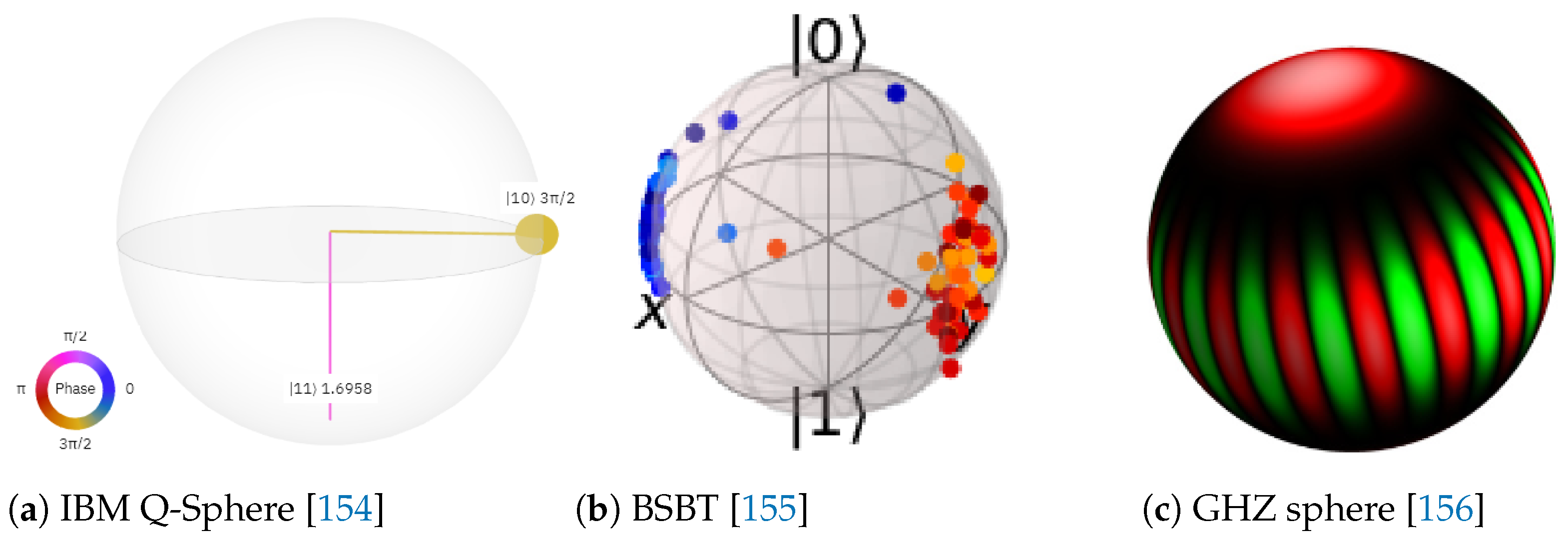
Figure 2. Examples of Quantum State Visualizations.

Figure 2. Examples of Quantum State Visualizations.

Unlike relational DBMSs, Array (Tensor) DBMSs manage multidimensional arrays (tensors) that often come from simulation outputs or diverse sensors. For example, Earth models (weather, climate, hydrology, etc.) or Earth observation. A numerical model can run on a quantum computer and load its output tensors into quantum memory. As the output tensors are already inside a quantum computer, Quantum Array (Tensor) DBMSs can perform operations on these output tensors without costly data movements between classical and quantum parts (components). Therefore, Array (Tensor) DBMSs have promise for practicality, especially for operating on tensors that are already in QRAM or RAQM (originated from a quantum algorithm or simulation).

In addition, note that the techniques presented further in this article are not completely tailored to quantum memory. If a multidimensional array (tensor) is already in a quantum register, as an output of some other quantum program, a Quantum Array (Tensor) DBMS can also be used to quickly operate on the quantum register that already contains data.

Just with 64 qubits we can address $2^{64}$ memory cells in a single quantum register. With additional 32 qubits for integer values, a quantum register ${\sum }_j{\psi }_j\left|j\right.〉\left|D_i\right.〉$ can store an array of 64 exbibytes (EiB) or over 73 exabytes (EB) of values, roughly $1000\times$ more than the entire Google Earth Engine platform to date [75], where $\left|j\right.〉$ and $\left|D_i\right.〉$ have 64 and 32 qubits respectively, 96 qubits in total. The data can be generated by a quantum algorithm and need efficient management by an Array (Tensor) DBMS, possibly entirely within a quantum computer. Recall that, to date, we already have real, working quantum computers with over 1000 qubits [92,157]. Optimistically, we can read $2^{64}$ QRAM cells in just $O\left(64\right)$ given appropriate hardware. With the vision on how to use quantum memory benefits, this article may additionally stimulate further quantum memory advancements.

2.3. Visualization in Quantum Computing

Let us summarize visualization techniques that facilitate working with quantum information to justify the introduction of our new quantum charts.

• Vector notation represents a state of single qubit quite well: ${\left[\begin{array}{cc}\alpha & \beta \end{array}\right]}^T$. However, as the number of qubits for visualization grows, the size of the resulting matrix grows exponentially and the vector notation becomes bulky and impractical:

  $$\left[\begin{array}{c}{\alpha }_1\\ {\beta }_1\end{array}\right]\otimes \left[\begin{array}{c}{\alpha }_2\\ {\beta }_2\end{array}\right]\otimes \cdots \otimes \left[\begin{array}{c}{\alpha }_n\\ {\beta }_n\end{array}\right]$$
• Dirac notation was developed, in particular, to address the aforementioned limitation of the vector notation. It is typical to write a superposition as a sum. However, it becomes hard to track the progression of the applied transformations. For example, which parts of the sum generated the subsequent parts in Equation (2) which has only three summands and one transformation. The growth of the transformation chain and the number of summands hinder the comprehension of the situation.
• Bloch sphere displays the state of only a single qubit, Figure 1.
• IBM Q-sphere [158] was introduced to overcome the visualization limitation of the Bloch sphere. However, IBM Q-sphere visualizes only one state of a quantum register on a sphere, not the sequence of transformations, Figure 2a.
• GHZ state spherical phase spaces [156] visualize a family of many-body states on a sphere, Figure 2c. Although important, this type of visualization hides actual values of information.
• Majumdar-Ghosh model qubism representation [159] focuses on the same family of states as the previous approach, but utilizes 2-d grids for visualization.
• Bloch Sphere Binary Tree (BSBT) [155] is a powerful visualization technique that can display time evolution and even datasets, Figure 2b. However, it can show a bird’s-eye view of the patterns and omits specific dataset values.
• Quantum circuit diagram is a fundamental way to graphically illustrate a quantum program using a set of connected operators, Figure 3. Many exciting and powerful quantum circuit visualizers exist, for example, IBM Qiskit [160] and Quirk [161]. However, circuits display the sequence of operations, not the data flow, e.g., values of quantum registers and their source-target relationships.

3. Quantum Gantt Chart (QGantt)

Quantum Gantt Chart is a new type of charts that we propose. Almost all quantum operations are applied in parallel to an exponential number of values. In addition, quantum registers can contain data derived from algorithm outputs or obtained from quantum memory. To understand, it is important to see array values, e.g., $\left|A\left[x\right]\right.〉$. Operations with multiple arities also require clear visualizations. For example, joining arrays A and B, denoted by $A\bowtie B$ (Section 4.7). In such cases, it is also important to see how indexes of A and B correspond to each other in $A\bowtie B$.

A far more complex problem is to statically visualize, letting users to explore the chart at their own pace, which and how many values are processed in parallel, inputs/outputs (values, not qubits) of operations, their duration, order, and to clearly annotate all of them with what they are doing. Obviously, current approaches (Section 2.3) fall short of clearly showing all the aforementioned information. They do not visualize or describe the flow of quantum computations combined with the data flow.

QGantt is a simple yet very informative way to statically visualize diverse quantum programs, suitable not only to the memory and Array (Tensor) DBMS aspects. Unlike the Gantt chart, the vertical axis depicts input/output data items for operations. The horizontal axis shows time and the duration of operations. Data items processed in parallel are located in a single column, annotated with explanations. Data items for the next operation go to the next column. If there are several logical stages (see Equation (39) as an example), QGantt charts can form a Quantum Network Diagram, Section 5. An important property of the QGantt chart is that it is straightforward to extend it by or combine it with other visualization techniques, see Section 2.3.

In the article, we typeset QGantt charts in due to aesthetic reasons. However, it is possible to render QGantt charts in an ASCII art or HTML versions, which are very flexible, similar to the way quantum circuits are presented in popular frameworks [160,161]. An example of an ASCII art version of a QGantt chart is in Section 5.4. Graphs are also good for displaying QGantt charts for practical reasons: diverse software can be used to manipulate graphs interactively. We will present increasingly complex QGantt charts during the progression of this article. For now, consider the following examples. We show that QGantt charts can naturally complement existing visualization techniques, including algebraic expressions with vector or Dirac notation, spherical representations, as well as quantum circuits. QGantt charts can also be used autonomously without additional visualization techniques, because QGantt charts are self-contained. In some cases, for example for operations with quantum memory or other data-centric algorithms, a QGantt chart can be the first visualization tool to try.

3.1. QGantt: Reading Data from Quantum Memory

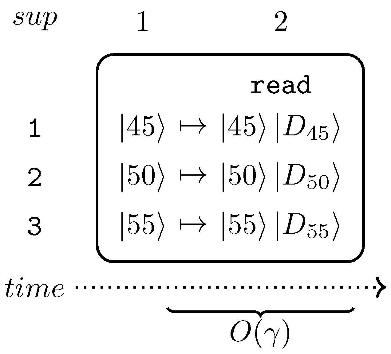
Let us refer to the algebraic description of how data is read from QRAM, Equation (2). The QGantt chart for Equation (2) looks much more clear, Figure 4. The chart omits ${\psi }_j$ as they are not important in this context. However, it is easy to add the values or visualizations (bars, circles, etc.) of ${\psi }_j$ if required.

Figure 4 provides a wealth of information. We see only one operation depicted in the QGantt chart: reading from QRAM. Therefore, the chart displays two main columns: the first column contains the terms that can be found in the superposition of the quantum register, and the second column provides the result. Note that the terms of a superposition are laid out vertically, representing the fact that they exist simultaneously, and an operation is applied to all the terms simultaneously as well.

The leftmost column contains the numbers of the superposition terms to facilitate referencing the terms. Significant columns or superposition columns (columns that contain terms that constitute a superposition, inputs or outputs) are numbered: see row $sup$ at the top. This makes it possible to reference any superposition term in a QGantt chart. For example, we can reference $\left|55\right.〉\left|D_{55}\right.〉$ just by $(3,2)$.

At the bottom, the timeline, together with braces, can provide an indication of the duration of each operation. Each operation has an underlying brace; the number of braces corresponds to the number of operations. Braces additionally help to visually separate operations from each other. Recall that in the case of reading from QRAM, the asymptotic runtime is logarithmic, and this is indicated under the brace: $\rho$ reads up to $2^{\gamma }$ cells in $O\left(\gamma \right)$, where $\gamma$ is the number of qubits for cell indexes in the quantum register, Table 1.

Finally, the name of an operation is placed above the column with the results of this operation, but below the column numbers. For example we see “read” which is the name of the operation (command) applied to the superposition in the first column and whose result (output) is in the column next to the input, the second column. Input terms point to the respective output terms with ↦ (arrow). The inputs and outputs of an operation can be surrounded with a box like in Figure 4 for the “read” operation to clearly attribute a block in a diagram to a certain operation. However, columns, rows, or regions in QGantt charts can be decorated in different ways as well.

3.2. QGantt: Creating Bell State

Bell state is a fundamental notion in quantum computing. Bell states are important for understanding superdense coding and quantum teleportation. Bell state demonstrates quantum entanglement [132,133,134,135,136]. The circuit that creates Bell state $\left|{\mathrm{\Psi }}^{+}\right.〉$ is in Figure 3. First, the Hadamard operator is applied to the first qubit. Then CNOT (Controlled NOT, Section 2.1) is used such that the first qubit is the control qubit.

The result of creating Bell state $\left|{\mathrm{\Psi }}^{+}\right.〉$ is the superposition of two entangled qubits: the outcome of the measurement of the first qubit is unknown and will result in 0 or 1 with the same probability equal to $1/2$. However, once the first qubit is measured, the measurement of the second qubit will always yield the same classical bit value equal to the measurement of the first qubit. This demonstrates quantum entanglement.

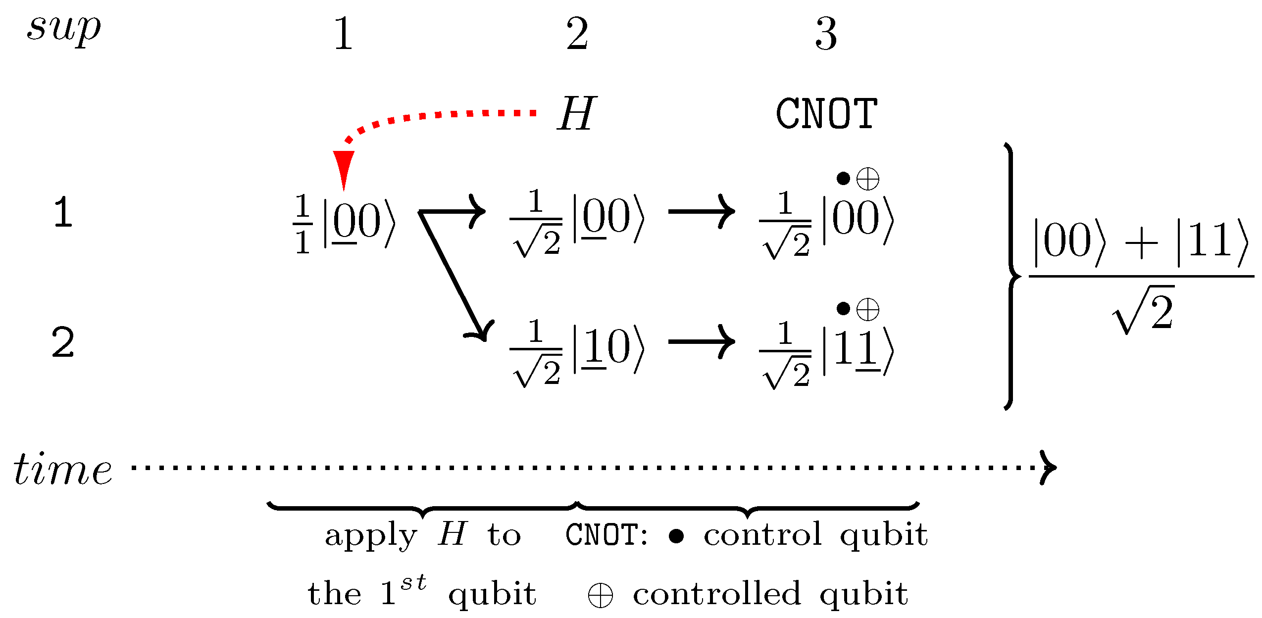
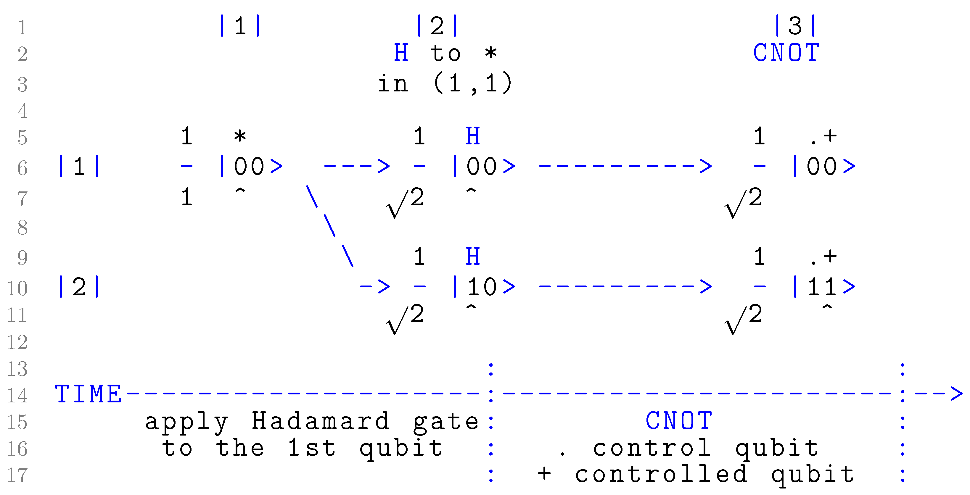
Let us show how QGantt charts excel in clearly visualizing, step-by-step, the creation of Bell state $\left|{\mathrm{\Psi }}^{+}\right.〉$, exact values of all intermediate states with their amplitudes, as well as their input/output relationships, Figure 5.

Figure 5 displays 3 superpositions in 3 columns. Any term in the diagram can be referenced by a row and column (superposition) number.

We start from the initial state $\left|00\right.〉$ with amplitude 1, where both qubits are initialized to $\left|0\right.〉$, Figure 5 $(1,1)$ (row № 1, column or superposition № 1).

At the next step, Hadamard gate is applied to the first qubit as shown by the red dotted line and pointed by the red arrow. The first qubit in $(1,1)$ is underlined to indicate that it participates in the operation. The red line, arrow and underlining are optional decorating elements to make the illustration more clear and apparent. The curly braces underneath indicate the scope of operations (inputs and outputs) and provide extra explanations.

After the application of Hadamard gate, we obtain two elements in the output superposition: $(1,2)$ and $(2,2)$ with the same amplitudes equal to $1/\sqrt{2}$. The amplitudes changed compared to the amplitude 1 of the input term $(1,1)$. Arrows pointing from $(1,1)$ to $(1,2)$ and $(2,2)$ indicate that both $(1,2)$ and $(2,2)$ resulted from an operation applied to a single term $(1,1)$.

Underlined qubits in $(1,2)$ and $(2,2)$ additionally emphasize that a modification or impact was caused to the underlined qubits compared to the previous superposition.

The last step is the application of the CNOT operation, column № 3. Symbols • and ⊕ mark the control and controlled qubits respectively. We could place these symbols somewhere at the top of $(1,3)$, as the positions of the control and controlled qubits are the same for each term in column № 3. However, symbols • and ⊕ appear over each term in the superposition, as many such terms can exist in a column and we should not scroll to find out which qubits are used for the CNOT operation and what their role is. The second value in $(2,3)$ is underlined as it was modified as a result of the CNOT operation: from 0 in $(2,2)$ to 1 in $(2,3)$.

Figure 5 shows the steps to create a Bell state with 2 qubits. It is straightforward to extend this diagram to illustrate the steps required to create a Greenberger–Horne–Zeilinger state (GHZ state) with 3 qubits: $(\left|000\right.〉+\left|111\right.〉)/\sqrt{2}$  [132,133,134,135,136]. For the purpose of a step-by-step illustration of creating the aforementioned GHZ state, symbols • and ⊕ for the CNOT operation will be much more necessary to increase clarity. For example, the notation $|1\stackrel{•}{1}\underline{\stackrel{\oplus }{1}}\rangle$ indicates that the CNOT operation was applied to the 2^nd and the 3^rd qubits, not some other combination of qubits, and the 3^rd qubit is underlined as it is that qubit that was modified in the result of the operation.

4. Quantum Array (Tensor) DBMS Techniques

4.1. Quantum Array (Tensor) Data Model

Now we carefully start defining the first quantum array (tensor) data model, as it will determine the overall Quantum Array (Tensor) DBMS design. To comply with state-of-the-art, we extend the formal model from [17].

4.1.1. Logical Array (Tensor)

An N-dimensional array (N-d array or tensor) is the mapping $A:D_1\times D_2\times \cdots \times D_N\mapsto \mathbb{T}$, where $N>0$, $D_i=[0,l_i)\subset \mathbb{Z}$, $0<l_i$ is a finite integer, and $\mathbb{T}$ is type. $l_i$ is said to be the size or length of ith dimension. Here and further on $i\in [1,N]\subset \mathbb{Z}$. Let us denote the N-d array (tensor) by

$$A\langle l_1,l_2,\dots ,l_N\rangle :\mathbb{T}$$

(3)

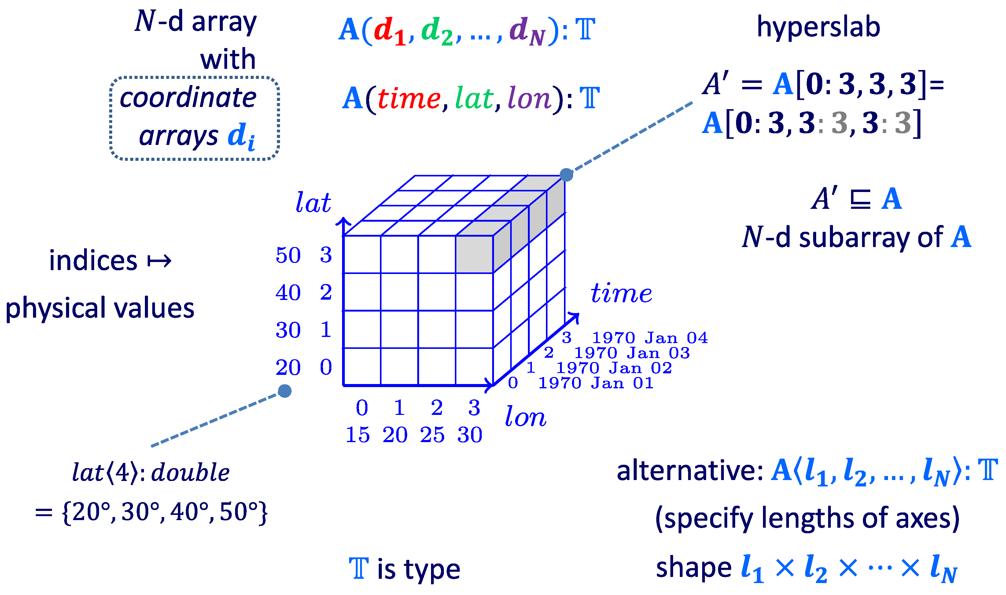
By $l_1\times l_2\times \cdots \times l_N$ denote the shape of A, by $\left|A\right|$ denote the size of A such that $\left|A\right|={\prod }_i{l}_i$. A cell or element value of A with integer indexes $(x_1,x_2,\dots ,x_N)$ is referred to as $A[x_1,x_2,\dots ,x_N]$, where $x_i\in D_i$. Each cell value of A is of type $\mathbb{T}$, Figure 6.

An array (tensor) may be initialized after its definition by enumerating its cell values. For example, the following defines and initializes a 2-d array (matrix) of integers: $A\langle 2,2\rangle :\mathbb{Z}$=$\left\{\right\{1,2\},\{\mathtt{NA},4\left\}\right\}$. In this example, $A[0,0]=1$, $A[1,0]=\mathtt{NA}$, $\left|A\right|=4$, and the shape of A is $2\times 2$. A missing value is denoted by NA. Other popular names for NA are null , NoData, n/a, NaN, and others.

Indexes $x_i$ are optionally mapped to specific values of ith dimension by coordinate arrays $A.d_i\langle l_i\rangle :{\mathbb{T}}_i$, where ${\mathbb{T}}_i$ is a totally ordered set, $d_i\left[j\right]<d_i[j+1]$, and $d_i\left[j\right]\ne \mathtt{NA}$ for $\forall j\in D_i$. In this case, A can be also defined as

$$A(d_1,d_2,\dots ,d_N):\mathbb{T}$$

(4)

Without loss of generality, in this article we will work with integer types of $\mathbb{T}$. Therefore, we will omit $\mathbb{T}$ if it is not important or we will write a numerical value instead of $\mathbb{T}$ to indicate the number of bits or qubits used to store an array value, e.g., $A\langle 2,2\rangle :q$, $q\in \mathbb{N}$.

Figure 6. An array (tensor) data model illustration.

Figure 6. An array (tensor) data model illustration.

A hyperslab$A^{\prime }⊑A$ is an N-d subarray of A. The hyperslab $A^{\prime }$ is defined by the notation

$$A[b_1:e_1,\dots ,b_N:e_N]=A^{\prime }(d_1^{\prime },\dots ,d_N^{\prime })$$

(5)

where $b_i,e_i\in \mathbb{Z}$, $0⩽b_i⩽e_i<l_i$, $d_i^{\prime }=d_i[b_i:e_i]$, $|d_i^{\prime }|=e_i-b_i+1$, and for all $y_i\in [0,e_i-b_i]$ the following holds:

$$\begin{array}{cc}\hfill A^{\prime }[y_1,\dots ,y_N]& =A[y_1+b_1,\dots ,y_N+b_N]\hfill \end{array}$$

(6a)

$$\begin{array}{cc}\hfill d_i^{\prime }\left[y_i\right]& =d_i[y_i+b_i].\hfill \end{array}$$

(6b)

Equations (6a) and (6b) state that A and $A^{\prime }$ have a common coordinate subspace over which cell values of A and $A^{\prime }$ coincide. The dimensionality of A and $A^{\prime }$ is the same. In hyperslab definitions, Equation (5), we will omit “$:e_i$” if $b_i=e_i$ or “$b_i:e_i$” if $b_i=0$ and $e_i=\left|d_i\right|-1$.

4.1.2. Quantum Model Aspects

Section 4.1.1 defines a logical array (tensor) whose model is common for classical and Quantum Array (Tensor) DBMSs. We further extend this model with quantum aspects for which the notations from Section 4.1.1 are also used. For example, we introduce quantum tensor strips (Section 4.5) and quantum hyperslabbing (Section 4.6) among other aspects. However, our extensions appear in the forthcoming sections to make the presentation and the justification for extensions more clear and timely. Hence, we first introduce our quantum memory operations and then describe our extensions to the array (tensor) model in the context of Array (Tensor) DBMS challenges. We mark model extensions with .

4.2. Array (Tensor)

To date, the R&D area of Array (Tensor) DBMSs is at the stage of forming its terminological dictionary. Moreover, it is a relatively young R&D area and no commonly accepted standards have been established for array (tensor) schema, query languages, the set of supported operations (operators), and many other Array (Tensor) DBMS aspects [7,8,9].

Array (Tensor) DBMSs operate on multidimensional arrays (tensors): the formal definition is in Section 4.1.1. However, here we additionally elaborate on the naming of this class of DBMSs: why do we use the word combination “Array (Tensor)”?

The history begins from Titan  [162] and Paradise  [163], one of the first database systems that specifically focused on array operations. They targeted Earth remote sensing data, as newly launched satellites challenged the data management community by generating massive amounts of data, mostly 2- and 3-dimensional arrays. At the time, this data was new to the DBMSs and fundamentally different from the other supported data types.

It was quickly realized that many core data types in numerous other domains are naturally modeled by multidimensional arrays (tensors). As 2-dimensional arrays were most common, even one of the earliest systems was called RasDaMan, which stands for “Raster Data Manager”. However, it was clear that an array database management system goes far beyond rasters. That was reflected in the names of subsequent systems, e.g., “A Multidimensional Array DBMS” [164] or “A query language for multidimensional arrays” [165].

Although the word “array” does not clearly reflect that a software system can work with an array with more than 2 dimensions, “multidimensional array” becomes a too lengthy term. Even worse, it is hard to translate “Array DBMS” in an awkward-free manner into other languages. For at least these two solid reasons, the term “Array DBMS” should be reconsidered.

Today, we believe that “Tensor DBMS” best reflects the essence of a database system that manages multidimensional arrays. The trend towards using the word “tensor” is strongly supported not only by the data management community, but also across a wider research environment [7,166]. For example, “tensors are natural multidimensional generalizations of matrices” and “by tensor we mean only an array with d indices” [166].

However, we are experiencing an intermediate period of the gradual transition to the name “Tensor DBMS”. Therefore, in this article, we still use the terms “Array (Tensor) DBMS” and “array (tensor)” for clarity as to which software systems and objects we refer to and to foster the transition.

The word “tensor” is increasingly used not only for an array with over two dimensions, but even for matrices (“2-d arrays” or “2-d tensors“) [167]. Technically and semantically, there is little or often no difference in how a state-of-the-art Array (Tensor) DBMS operates on a 1-dimensional, 2-dimensional, or an N-dimensional array where $N\in \mathbb{Z}$ and $N>2$ [7]. Consequently, we use the word combination “array (tensor)” or rarely one of these two words in our article.

Note that in our data model, a tensor is more than just an array with d indices, because it supports modeling of a wide variety of common and exotic Earth data types, including meshes, irregular grids, and others [17].

It is also worth mentioning that some researchers use the term “data cube” [35]. However, it is mostly understood as an object that can be obtained by issuing respective queries to an Array (Tensor) DBMS  [7].

Regardless of the current and possible future variations in the naming of database systems that manage diverse types of multidimensional arrays, and the naming of these arrays (rasters, tensors, data cubes, etc.), the word “tensor” perfectly reflects that an array can be multidimensional, is an international term, and is widely used in the research community directly for the purpose of referring to multidimensional arrays.

4.3. Illustrative Datasets

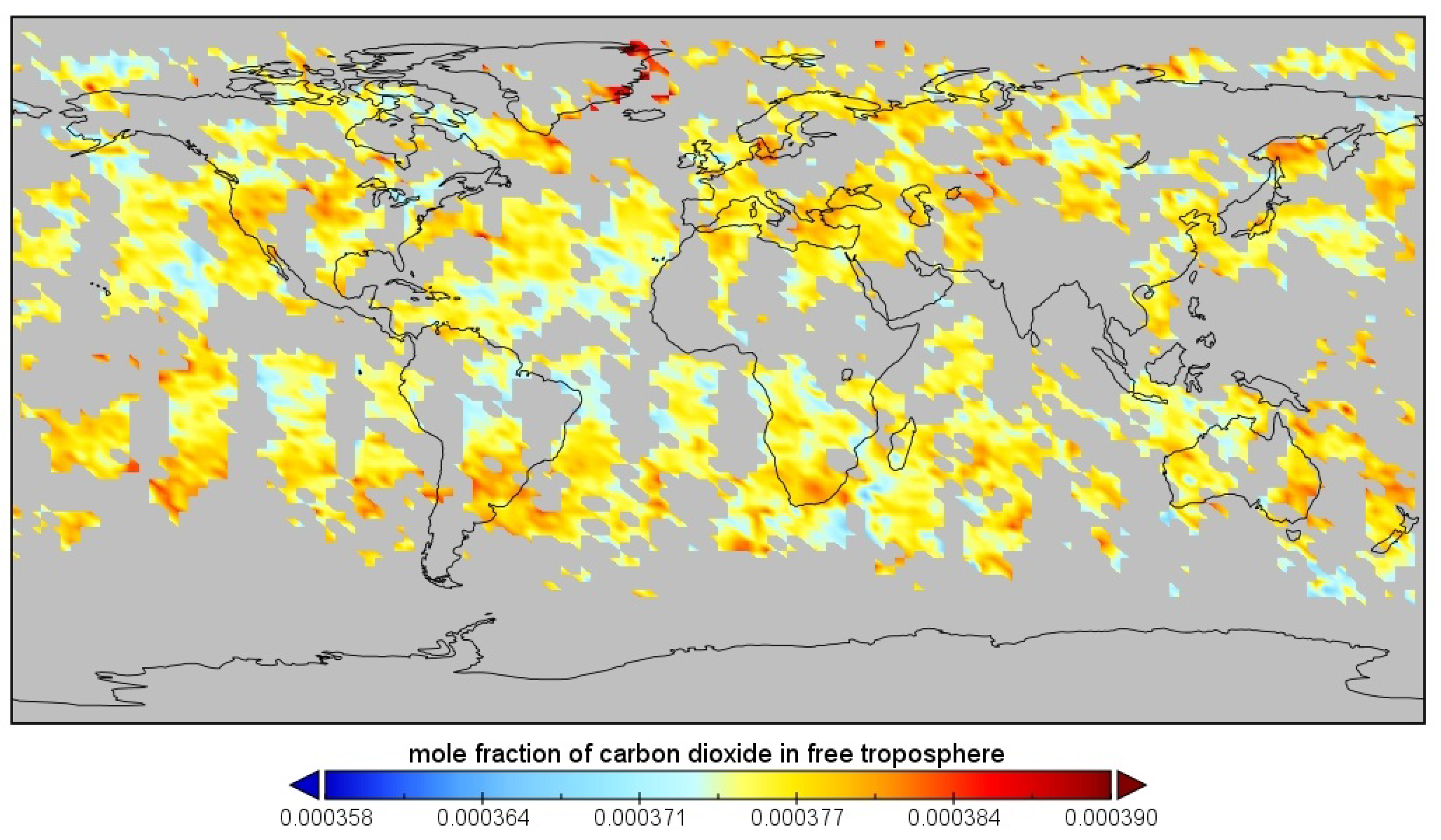
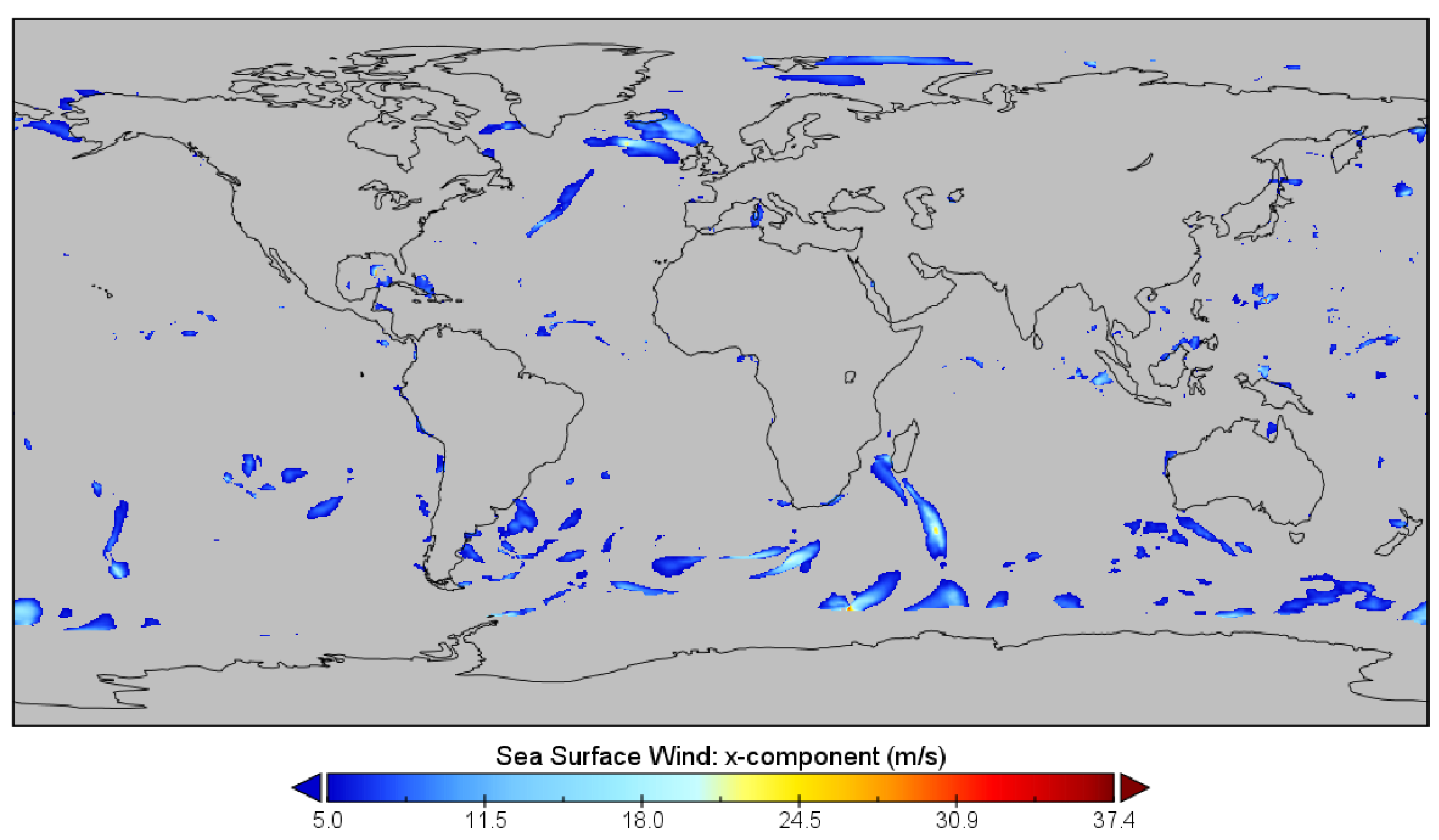
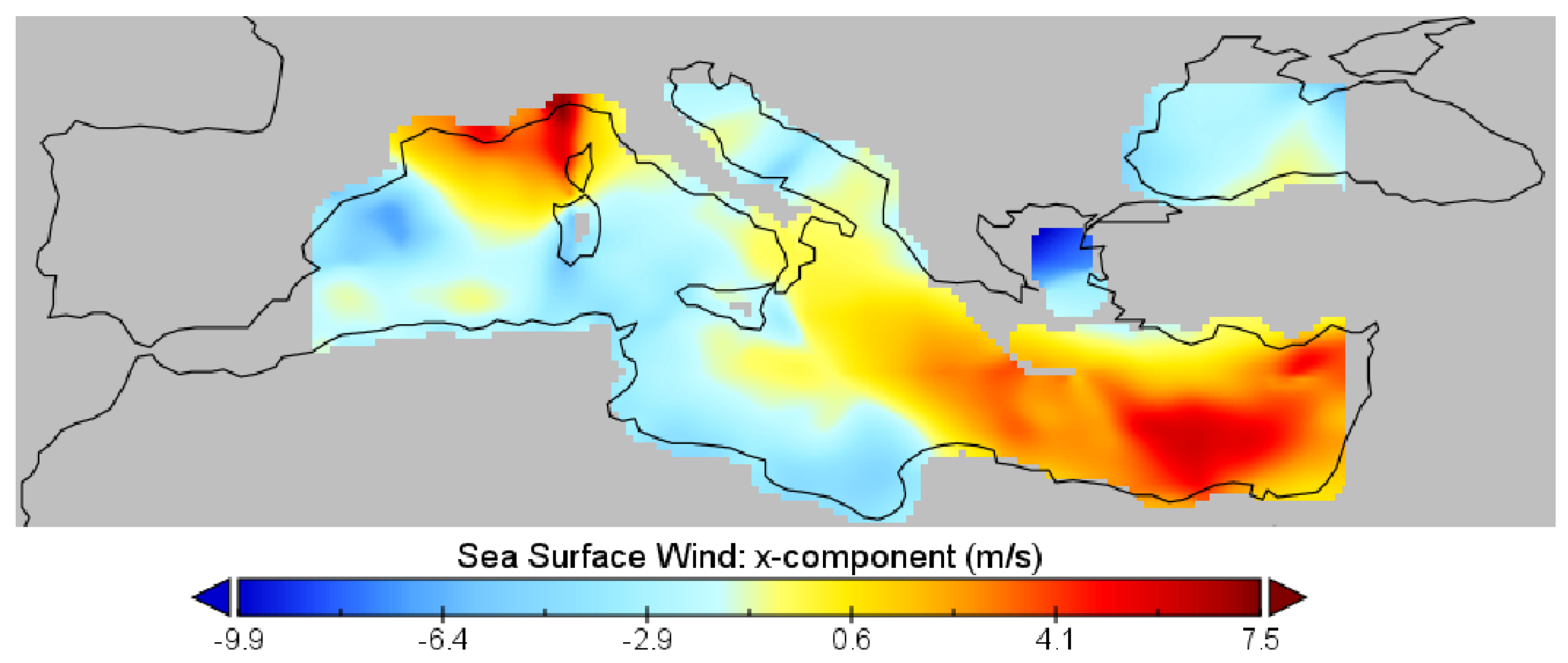
Let us take typical and popular Earth datasets that are subject to hyperslabbing, filtering, map algebra, and other operations that usually occur in Earth data engineering. We selected x-component of sea surface wind (Figure 7) and ${\mathrm{CO}}_2$ mole fraction (Figure 8) as motivating examples for a range of our quantum array (tensor) operations.

Let $W_{28}(la{t}_W,lo{n}_W)$ be the NOAA/NCDC sea surface wind speed array for the 28^th of August, 2005, Figure 7.

$$\begin{array}{ccc}\hfill {lat}_W\langle 719\rangle & =\{-89.75,-89.50,\dots ,89.75\}\hfill & \hfill +0.25°\mathrm{step}\\ \hfill {lon}_W\langle 1440\rangle & =\{0.00,0.25,\dots ,359.75\}\hfill & \hfill +0.25°\mathrm{step}\mathrm{as}\mathrm{well}\end{array}$$

(7)

Therefore, the shape of $W_{28}$ is $719\times 1440$.

Figure 7. NOAA/NCDC blended 6-hr 0.25° sea surface winds, 28 August 2005 ($719\times 1440$ cells).

Figure 7. NOAA/NCDC blended 6-hr 0.25° sea surface winds, 28 August 2005 ($719\times 1440$ cells).

Figure 8. AIRS-AMSU mole fraction of ${\mathrm{CO}}_2$ in free troposphere, 1 August 2004 ($91\times 144$ cells).

Figure 8. AIRS-AMSU mole fraction of ${\mathrm{CO}}_2$ in free troposphere, 1 August 2004 ($91\times 144$ cells).

Similarly, let ${\mathrm{CO}}_2^{01}\langle la{t}_{\mathrm{CO}},lo{n}_{\mathrm{CO}}\rangle$ be the AIRS-AMSU mole fraction of ${\mathrm{CO}}_2$ in free troposphere for the 1^st of August, 2004, Figure 8. Here

$$\begin{array}{ccc}\hfill lo{n}_{\mathrm{CO}}\langle 144\rangle & =\{89.5,88.0,86.0\dots ,-60.0\}\hfill & \hfill -2°\mathrm{step}\\ \hfill la{t}_{\mathrm{CO}}\langle 91\rangle & =\{-180,-177.5,\dots ,177.5\}\hfill & \hfill +2.5°\mathrm{step}\end{array}$$

(8)

Hence, the shape of ${\mathrm{CO}}_2^{01}$ is $91\times 144$. Note that $lo{n}_{\mathrm{CO}}\left[0\right]-lo{n}_{\mathrm{CO}}\left[1\right]\ne 2$, so the first two elements make the array irregular at the very beginning. It becomes regular afterwards.

We do not use the cell type in both cases, so we do not particularize $\mathbb{T}$.

4.4. Quantum Memory Operations

Memory is an essential component of a computing machine, but contemporary literature devotes little attention to the interactions of algorithms and quantum memory. Hence, one of the most important questions we start with is how memory can be organized for and accessed by a Quantum Array (Tensor) DBMS. This subsection contributes by reasoning about quantum array-tailored memory operations, as current literature lacks these aspects.

To move further, we need to introduce memory operations and reason about their costs. Let us denote by $\rho$ and $\omega$ read and write memory operations respectively, by $\pi$ we denote a quantum pointer ${\sum }_j{\psi }_j\left|j\right.〉$. Then $\rho \left(\pi \right)={\sum }_j{\psi }_j\left|j\right.〉|D_j\rangle$, where $D_j$ is the value of the jth memory cell [145]. We do not make assumptions on whether $\rho$ destroys memory cells after the completion of the operation. However, the property of being non-destructive would be very beneficial such that source tensor values do not vanish once they are read. We assume that we can perform several read and write operations in the same algorithm.

Note that $\pi$ does not necessarily address continuous memory cells. Let us assume that a quantum pointer $\pi$ has $\gamma$ qubits. Similarly, $\omega \left({\sum }_j{\psi }_j\left|j\right.〉\right|D_j\rangle )$ writes into quantum memory value $D_j$ to the jth memory cell for each j.

Next, let us assume that read and write operations on QRAM and RAQM are reversible, i.e., $A=\rho \left(\pi \right)$ after the following sequence of operations: $A\leftarrow \rho \left(\pi \right)$ and $\omega \left(A\right)$. We do not require that ${\psi }_j$ are the same after a sequence of the read and write operations, only pairs $\left|j\right.〉|D_j\rangle$ are the same. We can expect

$$\pounds \left(\rho \right(\pi \left)\right)=\pounds \left(\omega \right(\rho \left(\pi \right)\left)\right)=O\left(n\right)$$

where $\left|\{\forall j\}\right|=2^n$ and £ denotes asymptotic cost (recall that symbols T and $\mathbb{T}$ are already reserved), Section 6.1.6. In other words, $\pounds \left(\rho \left(H^{\otimes n}{\left|0\right.〉}^{\otimes n}\right)\right)=O\left(n\right)$. This will enable efficient implementations of many quantum algorithms, for example, the Grover search algorithm, HHL for Linear Algebra, Quantum Fourier Transform, pattern recognition, and others, yielding exponential speedups [141,145].

We have already illustrated reading from QRAM in Figure 4.

Note that in Section 4.7 we further extend $\rho$ to retrieve cell indexes from the first $\gamma$ qubits of a superposition. We present the extension and an important use case in Section 4.7.

4.4.1. NA in Tensor Cell Values

An interesting question is whether we should read and write $\left|D_j\right.〉$ values that are equal to $\left|\mathtt{NA}\right.〉$, i.e., the way how to handle the term ${\psi }_j\left|j\right.〉\left|\mathtt{NA}\right.〉$. The most appropriate implementation for $\rho$ is to skip NA cell values, but this may pose engineering challenges. In this case, the input to $\rho$ could be a starting memory cell index s and length n (the number of cells to be read) rather than a quantum pointer: $\rho (s,n)={\sum }_j{\psi }_j\left|j\right.〉|D_j\rangle$, where $D_j$ is the value of the jth memory cell such that $D_j\ne \mathtt{NA}$ and $j\in [s,s+n]$ (no terms in superposition with missing values), $n\in \mathbb{N}$. This will automatically enable intrinsic tensor compaction (Section 4.5).

This formulation seems simpler compared to submitting a superposition to $\rho$, because $\rho$ takes just 2 values and generates a superposition itself. Although it may be possible to parameterize $\rho$ in this way, the runtime cost need to be clarified for this setup: the worst case is $O\left(n\right)$ as for the classical memory. A good cost is $O(logn)$.

We analyze an important scenario where it can be beneficial, but not strictly necessary to eliminate NA cell values in Section 4.5. In the same section we also present an approach to remove NA cell values from an arbitrary quantum register, using quantum memory. The approach does not require additional hardware support for skipping NA cells in $\rho$, Section 4.5.4. If RAQM is available, we can easily construct a superposition for $\rho$ that does not contain cell indexes which point to NA values, see also Section 4.5.4.

4.4.2. NA in Address Indexes

A similar question is whether we should also allow a quantum register to contain ${\psi }_j\left|\mathtt{NA}\right.〉|D_j\rangle$ (NA as a cell index). We discuss a specific and important use-case where it is reasonable to have NA as an address (index) for an array (tensor) cell and which can benefit from specific handling of NA in cell indexes at the hardware level in Section 5.2.

At the hardware level, it would be perfect if $\rho$ and $\omega$ omit cells indexed with NA: ${\psi }_j\left|\mathtt{NA}\right.〉\mapsto {\psi }_j\left|\mathtt{NA}\right.〉\left|\mathtt{NA}\right.〉$ for $\rho$ and $\omega$ skips ${\psi }_j\left|\mathtt{NA}\right.〉|D_j\rangle$. Another solution is just to use the fact that NA can be a usual constant value, for example $2^{\left|\mathbb{T}\right|}-1$ for an array $A\langle d\rangle$, where $d\langle \rangle :\mathbb{T}$. In this case, before invoking $\rho$ or $\omega$, it is possible to replace NA with some dummy index such that $\rho$ reads the same value addressed by NA while $\omega$ writes all values to some dummy index (if parallel writes to the same index are supported). Again, before writing or reading, it is possible to utilize the NA elimination technique to avoid parallel writes to the same address or redundant reads from multiple dummy indexes, Section 4.5.4.

4.5. Quantum Sparse Arrays (Tensors)

Recall that an N-d array (tensor) can have missing values denoted by NA, Section 4.1.1. In general, the distribution of NA values seems random and may change after updates. Classically, memory space, I/O and CPU time are often wasted on NA-related issues. Many techniques tackle the problems of sparse arrays, e.g., TileDB has a new on-disk format with support for fast updates [56] and SciDB provides ragged arrays [67]. However, with classical memory, efficient storage and transformation of such arrays for diverse workloads becomes a Holy Grail  [7,66].

Sparse arrays are quite common in Earth data engineering. For example, Figure 7 provides no sea surface wind speed values for land which constitutes about $29\%$ of Earth’s surface. Hence, the wind speed array can be considered as a sparse array. Although array cells that correspond to land are predictable, more complex cases exist. Earth remote sensing data products can contain missing values in hardly predictable areas for each array. For instance, consider mole fraction of ${\mathrm{CO}}_2$ in free troposphere, Figure 8.

Classical Challenge 1. How to efficiently represent sparse arrays (arrays with a large number of NA values)?

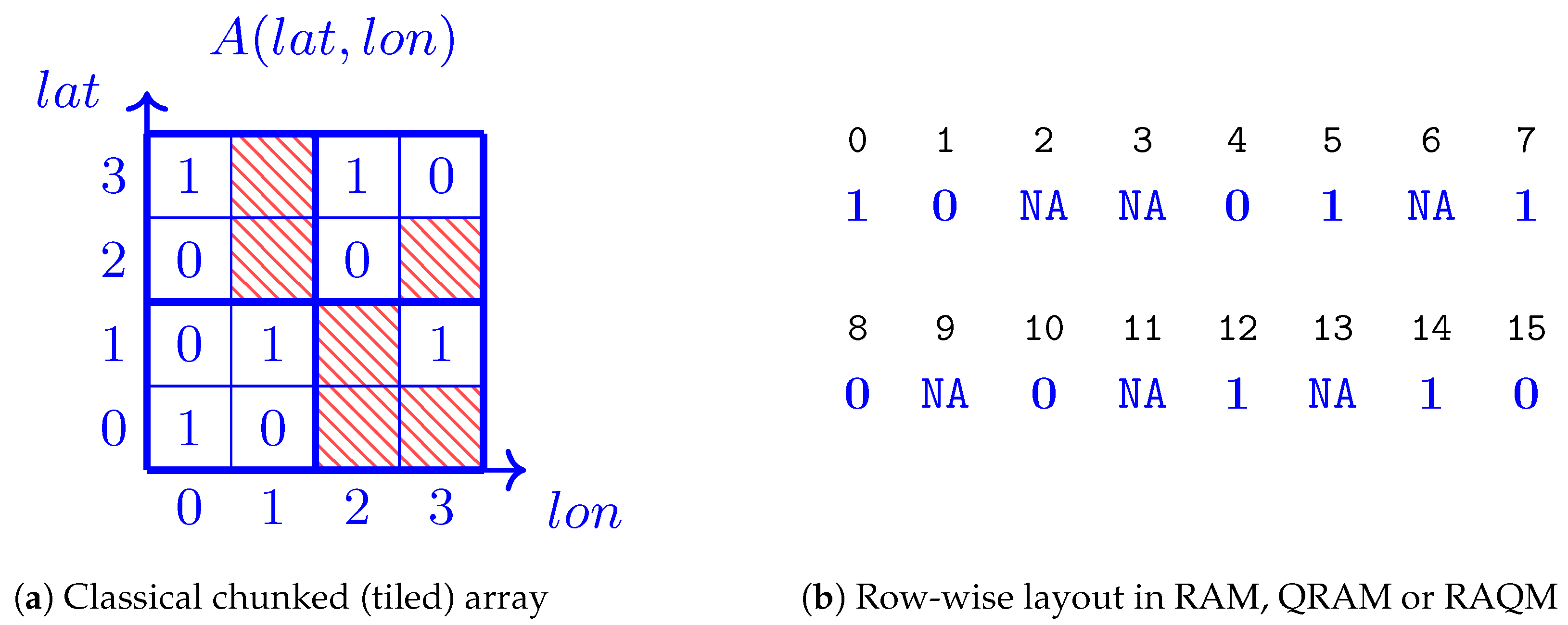
To make the discussion more specific with concrete numbers, consider an array $A(lat,lon):\mathbb{T}$ such that $\left|A\right|=16$, $\left|lat\right|=\left|lon\right|=4$, Figure 9a. Array A has 16 cells and 6 cells (dashed red lines) do not contain values (NA cells, technically these cells can contain a special constant that denotes a missing value). Other values are numbers 0 or 1.

A classical solution to the stated challenge is to split an array into chunks or tiles: I/O units used to read/write array portions, Figure 9a. Typically, a classical array is processed (i.e., read, write, filter cells) in chunks or tiles which are smaller subarrays. Thick blue lines in Figure 9a separate chunks from each other. Chunks make array processing more manageable and avoid reading the whole array into the operating memory.

This approach works good for dense arrays (with little number of NA values), but becomes inefficient for sparse arrays which have many NA values. For example, consider chunk (subarray) $A[0:1,2:3]$. It contains only one value at $A[1,3]$ and the other cells are empty. Allocating, reading, and writing a chunk of 4 cells leads to wasting $75\%$ of resources. Of course, Figure 9a represents a tiny example to facilitate understanding. Typical 2-d chunk shapes can be $512\times 512$ and similar. Chunking is usually applied to arrays in persistent storage like SDD or Amazon S3. For classical RAM, the basic storage schemes are row-wise (Figure 9b) or column-wise layouts. However, to increase array processing efficiency, sophisticated RAM layouts are also devised, e.g., Apache Arrow [168].

Quantum Look at Challenge 1. A Quantum Array (Tensor) DBMS Data Model is a radical departure from a classical array data model which splits a large Nd array into multiple chunks or tiles to create a more manageable dataset. Quantum Array (Tensor) DBMSs can now operate on quantum strips, or simply strips, Section 4.5.1 and Section 4.5.2. We introduce a new term, quantum strips, to clearly distinguish quantum array (tensor) formats (layouts) from chunks, tiles, and other classical entities.

4.5.1. Wide Quantum Strips

An array A is represented as a wide quantum strip as follows:

$$A\langle l_1,l_2,\dots ,l_N\rangle =\sum _j{\psi }_j\left|x_1\right.〉\left|x_2\right.〉\dots \left|x_N\right.〉\left|A[x_1,x_2,\dots ,x_N]\right.〉$$

(9)

This array layout intrinsically enables efficient packing of both dense and sparse arrays and naturally or directly exposes array cells as inputs to quantum algorithms. While we can still use the classical data model described above to define inputs/outputs for Array (Tensor) DBMS approaches, we now operate on the quantum array (tensor) layout.

The wide quantum strip of array A in Figure 9a, but without NA cells, now looks like

$$\begin{array}{cc}\hfill A(lat,lon)\phantom{.}=\phantom{.}& {\psi }_{0,0}\left|0\right.〉\left|0\right.〉\left|1\right.〉+{\psi }_{0,1}\left|0\right.〉\left|1\right.〉\left|0\right.〉+\hfill \\ \hfill & {\psi }_{1,0}\left|1\right.〉\left|0\right.〉\left|0\right.〉+{\psi }_{1,1}\left|1\right.〉\left|1\right.〉\left|1\right.〉+{\psi }_{1,3}\left|1\right.〉\left|3\right.〉\left|1\right.〉+\hfill \\ \hfill & {\psi }_{2,0}\left|2\right.〉\left|0\right.〉\left|0\right.〉+{\psi }_{2,2}\left|2\right.〉\left|2\right.〉\left|0\right.〉+\hfill \\ \hfill & {\psi }_{3,0}\left|3\right.〉\left|1\right.〉\left|1\right.〉+{\psi }_{3,2}\left|3\right.〉\left|2\right.〉\left|1\right.〉+{\psi }_{3,3}\left|3\right.〉\left|3\right.〉\left|0\right.〉\hfill \end{array}$$

(10)

The same wide quantum strip of array A in Figure 9a, but with with NA values, looks like as follows:

$$\begin{array}{cc}\hfill A(lat,lon)\phantom{.}=\phantom{.}& {\psi }_{0,0}\left|0\right.〉\left|0\right.〉\left|1\right.〉+{\psi }_{0,1}\left|0\right.〉\left|1\right.〉\left|0\right.〉+{\psi }_{0,2}\left|0\right.〉\left|2\right.〉\left|\mathtt{NA}\right.〉+{\psi }_{0,3}\left|0\right.〉\left|3\right.〉\left|\mathtt{NA}\right.〉+\hfill \\ \hfill & {\psi }_{1,0}\left|1\right.〉\left|0\right.〉\left|0\right.〉+{\psi }_{1,1}\left|1\right.〉\left|1\right.〉\left|1\right.〉+{\psi }_{1,2}\left|1\right.〉\left|2\right.〉\left|\mathtt{NA}\right.〉+{\psi }_{1,3}\left|1\right.〉\left|3\right.〉\left|1\right.〉+\hfill \\ \hfill & {\psi }_{2,0}\left|2\right.〉\left|0\right.〉\left|0\right.〉+{\psi }_{2,1}\left|2\right.〉\left|1\right.〉\left|\mathtt{NA}\right.〉+{\psi }_{2,2}\left|2\right.〉\left|2\right.〉\left|0\right.〉+{\psi }_{2,3}\left|2\right.〉\left|3\right.〉\left|\mathtt{NA}\right.〉+\hfill \\ \hfill & {\psi }_{3,0}\left|3\right.〉\left|0\right.〉\left|1\right.〉+{\psi }_{3,1}\left|3\right.〉\left|1\right.〉\left|\mathtt{NA}\right.〉+{\psi }_{3,2}\left|3\right.〉\left|2\right.〉\left|1\right.〉+{\psi }_{3,3}\left|3\right.〉\left|3\right.〉\left|0\right.〉\hfill \end{array}$$

(11)

Now the aforementioned metrics for classical arrays (tensors) like $\left|A\right|$ do not reveal the quantum resource usage complexity. Let us denote by $\wr A\wr$ the number of qubits to keep the whole A in a quantum register. What is the order of $\wr A\wr$?

For a wide strip layout (this subsection), to keep in a quantum register a dense or sparse Nd array A that can contain from 0 up to $2^{N\gamma }$ cells of type $\mathbb{T}$ and the size of any dimension of A is no larger than $2^{\gamma }$, we need a quantum register with at least $\wr A\wr =\left|\mathbb{T}\right|+N\gamma$ qubits.

For a narrow strip layout (Section 4.5.2), to keep in a quantum register a dense or sparse array A that can contain from 0 up to $2^{\gamma }$ cells of type $\mathbb{T}$ (regardless of the dimensionality of A), we need a quantum register with at least $\wr A\wr =\left|\mathbb{T}\right|+\gamma$ qubits.

What is the quantum memory consumption for storing a dense or sparse array A?

If RAQM is used, we need the same number $\wr A\wr$ of qubits as for a quantum register to keep A in RAQM in Equation (10) or Equation (11), regardless of whether we have NA values in a strip or not. Moreover, if $\gamma$ qubits are used for a quantum pointer, and $\left|\mathbb{T}\right|$ qubits for a cell value of A, in the same RAQM cell of $\wr A\wr =2\times \gamma +\left|\mathbb{T}\right|$ qubits, we can store any 2d array from 0 up to $2^{2\times \gamma }$ cells of type $\mathbb{T}$. We do not need to devise compaction or packing schemes for arrays (tensors) of any dimensionality for RAQM to save space. A processing operation on such a strip will also require time proportional to $\wr A\wr$ regardless of an array (tensor) size. A sufficiently large $\gamma$ must be supported by RAQM to keep the whole array (tensor) in a single cell. Otherwise, an array (tensor) must be split and respective array (tensor) partitioning techniques for RAQM will be required, Section 6.1.3.

If QRAM is used, we may need the same number of cells $\left|A\right|$ to store array A similar to the classical model. Logically, QRAM can be similar to a row-wise layout. Figure 9b locates A values in a single row split into two rows. The numbers in the top row are cell indexes, while the numbers below indexes are the respective cell values (colored blue). At a glance, there is no benefit of using QRAM for storing arrays. In terms of occupied space, QRAM is not more optimal compared to classical RAM. However, an appropriate QRAM can be able to provide the following very attractive benefits:

• read A in $O\left(n\right)$ for $\left|A\right|=2^n$ or in $O(log|A\left|\right)$ compared to $O\left(2^n\right)$ for the classical case: an exponential speedup
• read arrays of significantly different sizes with almost the same performance: $O\left(64\right)$ may not be too different from $O\left(32\right)$ given the appropriate hidden constants
• atomically read any list of indexes in a single go by providing a superposition of QRAM indexes for $\rho$
• atomically write/update any list of values indexed by a superposition which can contain non-continuous index values

All of the above can be taken into consideration to develop appropriate algorithms for Quantum Array (Tensor) DBMSs.

4.5.2. Narrow Quantum Strips

Although $\left|x_1\right.〉\left|x_2\right.〉\dots \left|x_N\right.〉$ can be convenient for algorithms, it may pose significant requirements for a very large N. An alternative quantum array layout can look as a potentially more compact 1-d indexed strip:

$$A\langle l_1,l_2,\dots ,l_N\rangle =\sum _j{\psi }_j\left|j\right.〉\left|A[x_1,x_2,\dots ,x_N]\right.〉,\mathrm{where}j=\sum _{i=1}^{N-1}{x}_i{l}_i+x_N$$

(12)

Here $\left|j\right.〉$ is a 1-d index of an array cell A. We computed $\wr A\wr$ in Section 4.5.1. It is straightforward to convert a 1-d index to a sequence of values to form a higher-dimensional index. Now narrow $\wr A\wr$ can be less than wide $\wr A\wr$, but the burden of index conversion, although straightforward, can fall on oracles. For the RAQM and QRAM cases, the benefits of using narrow strips are similar as for using wide strips, but can depend on $\wr A\wr$.

As we have already noted, we need a new name for the quantum layouts: “strip” to emphasize its difference compared to chunks or tiles. Recall that we call layouts in Equations (9) and (12) as wide and narrow layouts respectively. Both layouts can be used for different purposes and new ones can also be devised.

In addition, note that QGantt chats visualize strips very clearly and explicitly, for example in Figure 4. Hence, besides other aspects, QGantt charts are also appropriate for investigating quantum memory and Quantum Array (Tensor) DBMS aspects.

4.5.3. Quantum Strip Layouts

In this article, we start from basic in-memory array (tensor) layouts due to the following reasons. First, state-of-the-art literature has almost no ideas on the algorithmic aspects of using quantum memory, as we have already noted. Second, before we move to advanced in-memory array (tensor) packing or compaction techniques, we must carefully investigate the advantages and disadvantages of a basic layout. Therefore, we start from QRAM (the most challenging compared to RAQM) and the row-wise layout that contains NA values (Figure 9b).

Recall the two interesting questions on whether we should allow NA in cell indexes (Section 4.4.2) and/or in cell values (Section 4.4.1). In general, we can store NA values in QRAM. Due to the logarithmic cost of $\rho$, there is no point in applying any array compaction schemes as they will not change the I/O memory runtime significantly unless we care about the memory footprint. We leave devising advanced array layouts for future work.

However, $\rho$ and any operation can produce NA in a strip. We may (1) do not care and skip NA values in algorithms, or (2) utilize NA elimination techniques to cleanup a strip to simplify its subsequent processing. If hidden constants in $\pounds \left(\rho \right)$ or $\pounds \left(\omega \right)$ are high, NA elimination will also be useful for reducing I/O time.

4.5.4. NA Elimination Technique (Deleting Terms from Quantum Superposition)

Let us present a technique to remove terms that satisfy a predicate from a quantum superposition. It is an important auxiliary operation that can be applied to a strip to avoid NA in an index or value. Ideas from this technique are also used in other Quantum Array (Tensor) DBMS approaches, including quantum array indexing algorithms (Section 4.9).

The problem statement is as follows. Without loss of generality, a narrow quantum strip comes as input, Equation (12). The approach is straightforward to extend to wide quantum strips, Equation (9). A narrow quantum strip without terms ${\psi }_j\left|j\right.〉\left|\mathtt{NA}\right.〉$ comes as output. For example, consider array $A(lat,lon)$, Equation (11). Let us rewrite its definition in a narrow fashion that corresponds to the row-wise layout in Figure 9b:

$$\begin{array}{cc}\hfill A(lat,lon)\phantom{.}=\phantom{.}& {\psi }_0\left|0\right.〉\left|1\right.〉+{\psi }_1\left|1\right.〉\left|0\right.〉+{\psi }_2\left|2\right.〉\left|\mathtt{NA}\right.〉+{\psi }_3\left|3\right.〉\left|\mathtt{NA}\right.〉+\hfill \\ \hfill & {\psi }_4\left|4\right.〉\left|0\right.〉+{\psi }_5\left|5\right.〉\left|1\right.〉+{\psi }_6\left|6\right.〉\left|\mathtt{NA}\right.〉+{\psi }_7\left|7\right.〉\left|1\right.〉+\hfill \\ \hfill & {\psi }_8\left|8\right.〉\left|0\right.〉+{\psi }_9\left|9\right.〉\left|\mathtt{NA}\right.〉+{\psi }_{10}\left|10\right.〉\left|0\right.〉+{\psi }_{11}\left|11\right.〉\left|\mathtt{NA}\right.〉+\hfill \\ \hfill & {\psi }_{12}\left|12\right.〉\left|1\right.〉+{\psi }_{13}\left|13\right.〉\left|\mathtt{NA}\right.〉+{\psi }_{14}\left|14\right.〉\left|1\right.〉+{\psi }_{15}\left|15\right.〉\left|0\right.〉\hfill \end{array}$$

(13)

The strip in Equation (13) contains NA values which should be excluded from the resulting strip (amplitudes may change):

$$\begin{array}{cc}\hfill A(lat,lon)\phantom{.}=\phantom{.}& {\psi }_0^{\prime }\left|0\right.〉\left|1\right.〉+{\psi }_1^{\prime }\left|1\right.〉\left|0\right.〉\hfill \\ \hfill & {\psi }_4^{\prime }\left|4\right.〉\left|0\right.〉+{\psi }_5^{\prime }\left|5\right.〉\left|1\right.〉+{\psi }_7^{\prime }\left|7\right.〉\left|1\right.〉+\hfill \\ \hfill & {\psi }_8^{\prime }\left|8\right.〉\left|0\right.〉+{\psi }_{10}^{\prime }\left|10\right.〉\left|0\right.〉\hfill \\ \hfill & {\psi }_{12}^{\prime }\left|12\right.〉\left|1\right.〉+{\psi }_{14}^{\prime }\left|14\right.〉\left|1\right.〉+{\psi }_{15}^{\prime }\left|15\right.〉\left|0\right.〉\hfill \end{array}$$

(14)

We have previously noted that we may need the removal of terms with NA in indexes or values for convenience of algorithms or possible reduction of load on $\rho$ and $\omega$, Section 4.5.3.

The removal of an arbitrary term from an arbitrary superposition is not trivial. If we just remove a term without adjusting amplitudes of other terms, the following condition will not hold and the algorithm will not work in a quantum computer: ${\sum }_k|{\psi }_k{|}^2={\sum }_j{\left|{\psi }_j^{\prime }\right|}^2=1$. According to a recent survey [169], only one algorithm exists to near completely delete a term from a superposition [170]. However, as can be concluded from the previous sentence, a complete deletion is not guaranteed. The approach [170] has the following limitations. The algorithm [170]:

• removes only 1 term at a time, but we need to remove all terms with NA and we do not know the quantity of such NA terms
• assumes that all terms are present in the superposition (for $\gamma$ qubits there should be $2^{\gamma }$ terms in the input superposition): in a quantum strip we may not have all terms after a sequence of operations or just because its length is less than $2^{\gamma }$ and is generally unknown
• assumes that the terms have the same amplitudes (${\psi }_j={\psi }_p$ for $\forall j,p$ and $j\ne p$) which may not hold and is hard to guarantee in practice due to the aforementioned reasons
• needs to perform floating point operations which are hard to implement without bias; nearly complete deletion means that the certainty of the operation is less than 100% and, therefore, subsequent algorithms still need to account for the deleted value as if it was not deleted; in our case, algorithms must still do additional checks to avoid NA even after deleting them: this renders such a deletion operation pointless

Instead of tweaking the amplitudes to make terms with NA cell values negligible, the core idea behind our NA elimination technique is to replace index p and value NA in all terms ${\psi }_p\left|p\right.〉\left|\mathtt{NA}\right.〉$ with an index j and $value$ of some other term ${\psi }_j\left|j\right.〉\left|value\right.〉$ that is taken from the same strip, where $value\ne \mathtt{NA}$. Our algorithm utilizes QRAM.

Let us introduce some non-limiting assumptions before we present our approach. First, we will work with 1-based, not 0-based indexed arrays similar to Fortran and Pascal. This is not a limitation: we can use 1-based indexing or increment cell indexes by 1 before applying the NA elimination technique. Note that in this case we do not have a term ${\psi }_0\left|0\right.〉\left|·\right.〉$ in the input strip. Second, NA will be a constant value with 1 in each qubit, i.e., $\mathtt{NA}={\left|1\right.〉}^{\otimes \left|\mathbb{T}\right|}$. This is a standard practice in classical Array (Tensor) DBMSs. Finally, we take into account the properties of $\rho$ and $\omega$, Section 4.4. NA both in index and/or value can be sometimes beneficial. However, if we would like to remove all terms in a quantum strip $\mathbb{S}$ with NA in cell values, the algorithm is as follows:

• Write $\mathbb{S}$ into QRAM: $O(log|\mathbb{S}\left|\right)$
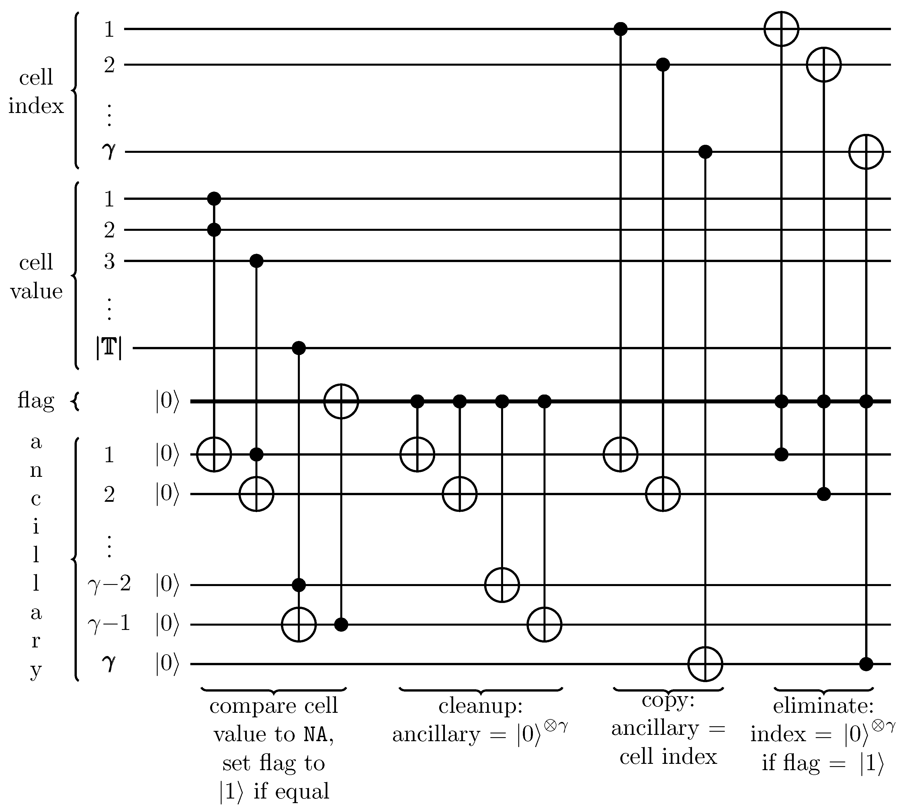
• Collapse all terms ${\psi }_p\left|p\right.〉\left|\mathtt{NA}\right.〉$ in the input strip $\mathbb{S}$ into a single term ${\psi }_0\left|0\right.〉\left|\mathtt{NA}\right.〉$ using the circuit in Figure 10: $O\left(\right|\mathbb{T}|+\gamma )$
• Perform the Quantum Amplitude Amplification (QAA) to decrease ${\psi }_0$ [171]: $O\left(\sqrt{\left|\mathbb{S}\right|}\right)$, heuristics can also be applied, see [171]
• Measure $\mathbb{S}$ to obtain any term ${\psi }_j\left|j\right.〉\left|value\right.〉$ where $value\ne \mathtt{NA}$: $O\left(1\right)$
• Read $\mathbb{S}$ from QRAM: $O(log|\mathbb{S}\left|\right)$
• Repeat step №2: $O\left(\right|\mathbb{T}|+\gamma )$
• Replace ${\psi }_0\left|0\right.〉\left|\mathtt{NA}\right.〉$ with ${\psi }_j\left|j\right.〉\left|value\right.〉$ using the same ideas as in the circuit in Figure 10: ${\psi }_0\left|0\right.〉\left|\mathtt{NA}\right.〉$ and ${\psi }_j\left|j\right.〉\left|value\right.〉$ will merge into $({\psi }_j+{\psi }_0)\left|j\right.〉\left|value\right.〉$, $O\left(\right|\mathbb{T}|+\gamma )$

Note that we can create a mask using strip $\mathbb{S}$ without NA values: we can create a superposition ${\sum }_j{\psi }_j\left|j\right.〉$ (without cell values), store it in a single RAQM cell, and read the strip from QRAM skipping cells that contain NA. Step №4 relies on the fact that ${\psi }_0$ will be very small. However, we must still check the $value$ after the measurement such that it is not equal to NA. Step №3 is the most time-consuming and challenging as it has a square root runtime. However, to date, it is the most generic way to de-amplify a superposition term.

The presented technique is flexible and can be plugged with another algorithm to find a term to use it to replace ${\psi }_0\left|0\right.〉\left|\mathtt{NA}\right.〉$. If we do use QAA, we may not collapse all terms with NA into a single term if we do not care about the impact on the $\omega$ operation or do not debug. However, if there is another heuristic algorithm that is faster than QAA in a particular setting and yields a term with $max$ index to use such a term to replace ${\psi }_0\left|0\right.〉\left|\mathtt{NA}\right.〉$, then we do need the collapsing procedure to guarantee that the index of NA is minimal. We may also skip step №6 by modifying step №7: replace all ${\psi }_p\left|p\right.〉\left|\mathtt{NA}\right.〉$ with ${\psi }_j\left|j\right.〉\left|value\right.〉$. Therefore, the presented algorithm is generic and can be configured according to the goals and available heuristics. Note that the circuit in Figure 10 is quite important in diverse settings. For example, ideas from this algorithm, and in particular the circuit in Figure 10, are used in Section 5.2 without QAA to efficiently answer both dimension- and value-based queries.

If we would like to save time, we may be satisfied with a compromise solution: keep NA in ${\psi }_0\left|0\right.〉\left|\mathtt{NA}\right.〉$ and do not seek another value to replace NA. We may already save time for $\omega$ as only 1 term with NA value will be written. Subsequent algorithms will need to skip only one term with an already known index 0 rather than checking each term for NA (quantum parallelism can skip every term with NA, but conceptually, it is easier to skip only one term than an unknown number of such). Finally, for some reason we may know a $value\ne \mathtt{NA}$ and its index, so it is possible to skip step №3.

To summarize, the asymptotic runtime cost of the NA elimination algorithm with all its steps is

$$\begin{array}{cc}\hfill \pounds \left(\mathtt{NA}\mathrm{eliminate}\mathrm{complete}\right)& =O(log|\mathbb{S}\left|\right)+O\left(\right|\mathbb{T}|+\gamma )+O\left(\sqrt{\left|\mathbb{S}\right|}\right)+O\left(1\right)+\hfill \\ \hfill & \phantom{=.}O(log|\mathbb{S}\left|\right)+O\left(\right|\mathbb{T}|+\gamma )+O\left(\right|\mathbb{T}|+\gamma )\hfill \\ \hfill & =O(log|\mathbb{S}\left|\right)+O\left(\right|\mathbb{T}|+\gamma )+O\left(\sqrt{\left|\mathbb{S}\right|}\right)\hfill \\ \hfill & =O(log|\mathbb{S}\left|\right)+O\left(\sqrt{\left|\mathbb{S}\right|}\right)=O\left(\sqrt{\left|\mathbb{S}\right|}\right)\hfill \end{array}$$

(15)

While getting $\pounds \left(\mathtt{NA}\mathrm{eliminate}\mathrm{complete}\right)=O\left(\sqrt{\left|\mathbb{S}\right|}\right)$ in Equation (15), we assume that although we need to perform read/write operations in $O(log|\mathbb{S}\left|\right)$, the execution of QAA in $O\left(\sqrt{\left|\mathbb{S}\right|}\right)$ time may still dominate the overall runtime, Section 6.1.6.

As noted above, if we omit steps №2 and №6, asymptotically we do not save time:

$$\begin{array}{cc}\hfill \pounds \left(\mathtt{NA}\mathrm{eliminate}\mathrm{reduced}\right)& =O(log|\mathbb{S}\left|\right)+O\left(\sqrt{\left|\mathbb{S}\right|}\right)+O\left(1\right)+\hfill \\ \hfill & \phantom{=.}O(log|\mathbb{S}\left|\right)+O\left(\right|\mathbb{T}|+\gamma )\hfill \\ \hfill & =O(log|\mathbb{S}\left|\right)+O\left(\right|\mathbb{T}|+\gamma )+O\left(\sqrt{\left|\mathbb{S}\right|}\right)\hfill \\ \hfill & =O(log|\mathbb{S}\left|\right)+O\left(\sqrt{\left|\mathbb{S}\right|}\right)=O\left(\sqrt{\left|\mathbb{S}\right|}\right)\hfill \end{array}$$

(16)

If we are satisfied with only 1 element to contain NA in its cell index, that is ${\psi }_0\left|0\right.〉\left|\mathtt{NA}\right.〉$, we need only step №2, which uses the circuit in Figure 10. In this case

$$\pounds \left(\mathtt{NA}\mathrm{eliminate}\mathrm{one}\right)=O\left(\right|\mathbb{T}|+\gamma )$$

(17)

which is the fastest version. The same asymptotic runtime applies to the case when a non-NA cell value and its index are known beforehand. Lastly, if there is a heuristic to find such index and value asymptotically faster than QAA, the asymptotic runtime depends on the complexity of that heuristic, but should be lower than $O\left(\sqrt{\left|\mathbb{S}\right|}\right)$.

The procedure for step №2 takes the superposition as input (pairs of cell values and indexes) and requires $\gamma +1$ ancillary qubits initialized to $\left|0\right.〉$, including a flag qubit and $\gamma$ qubits to perform the comparison and elimination, Figure 10.

The circuit in Figure 10 begins by comparing cell values to NA. It uses the Toffoli or CCNOT gate on 3 qubits. The controlled qubit (marked by ⊕) is inverted iff both control qubits (marked by •) are equal to $\left|1\right.〉$. Recall that NA consists entirely of qubits equal to $\left|1\right.〉$. Therefore, the ancillary qubit №1 will become $\left|1\right.〉$ iff both cell value qubit №1 and qubit №2 are $\left|1\right.〉$. As all cell value qubits should be equal to $\left|1\right.〉$ to represent the NA value, we involve the result of the previous CCNOT gate: ancillary qubit №1 together with cell value qubit №3 and so on. Ancillary qubit №$(\gamma -1)$ will be equal to $\left|1\right.〉$ if the cell value is NA. The diagram shows the most complex case when $\left|\mathbb{T}\right|=\gamma$. We copy the value of this qubit to the flag qubit as we will need ancillary qubit №$(\gamma -1)$ to copy cell index.

Afterwards, we cleanup all ancillary qubits by setting their values to $\left|0\right.〉$ using the CNOT gate and the flag as the control qubit. Then we copy the value of cell indexes to ancillary qubits with the CNOT gate. Finally, a series of $\left(\gamma \right)$ CCNOT gates with flag as one of the control qubits and each ancillary qubit, one by one, sets the cell index qubits to $\left|0\right.〉$ if the flag qubit is $\left|1\right.〉$ (the cell value is NA). If the flag qubit is $\left|1\right.〉$ and an ancillary qubit №i is also $\left|1\right.〉$, then cell index qubit №i is also $\left|1\right.〉$ as we have previously copied its value to ancillary qubit №i. Hence, cell index qubit №i will be inverted to $\left|0\right.〉$. Of course, no action will be taken if ancillary qubit №i is $\left|0\right.〉$, which is also equal to cell index qubit №i.

The circuit in Figure 10 runs in constant time $O\left(\right|\mathbb{T}|+\gamma )$: it requires $\left(\right|\mathbb{T}|+\gamma )$ CCNOT gates and $\left(\right|\mathbb{T}|+\gamma +1)$ CNOT gates.

4.6. Quantum Array (Tensor) Hyperslabbing

Hyperslabbing is a fundamental operation in Earth data engineering. For data in Figure 7 and Figure 8, hyperslabbing can help to select data within certain geographical areas.

For example, ${\mathrm{W}}_{28}[480:540,0:141]$ hyperslabs ${\mathrm{W}}_{28}$ (sea surface wind speed) for the area between 30°…45° N (latitudes) and 0°…35° E (longitudes) that approximately corresponds to the Mediterranean sea. Note that $la{t}_W\left[480\right]=30$, $la{t}_W\left[540\right]=45$, $lo{n}_W\left[0\right]=0$, and $lo{n}_W\left[141\right]=35$, Figure 11.

For an array (tensor) with more dimensions, e.g., time and/or height in addition to latitude and longitude, hyperslabbing can also extract a 3-d cube or an N-d array that corresponds to a given spatio-temporal interval.

Let us complement the model in Section 4.1.2 with quantum hyperslabbing using classical indexes (QHCI):

$$A[x_1^b:x_1^e,\dots ,x_N^b:x_N^e]\mapsto \sum _j{\psi }_j\left|x_1\right.〉\left|x_2\right.〉\dots \left|x_N\right.〉\left|A[x_1,x_2,\dots ,x_N]\right.〉$$

(18)

where $x_i\in [x_i^b,x_i^e]\subseteq D_i$ and $i\in [1,N]$. Despite the seemingly simple definition of hyperslabbing, its efficient execution is not simple at all: the performance varies by orders of magnitude depending on the array layout that is often tuned by trial & error [17].

Let us further complement the model in Section 4.1.2 with Quantum Hyperslabbing using Quantum Indexes (QHQI):

$$A[\overline{x_1},\dots ,\overline{x_N}]=\sum _j{\psi }_j\left|x_1\right.〉\dots \left|x_N\right.〉\left|A[x_1,x_2,\dots ,x_N]\right.〉$$

(19)

for each $x_i$ such that $|\langle x_i\left|\overline{x_i}\right.〉{|}^2\ne 0$ and $\overline{x_i}$ is a superposition of cell indexes that uses $\gamma$ qubits. The main difference of quantum indexes compared to classical indexes is that we can conveniently and concisely express non-continuous array (tensor) strips with quantum indexes. For example, consider an array $A\langle 3,3\rangle$. The following will extract 4 non-neighbor (non-continuous) values $A[0,0]$, $A[0,2]$, $A[2,0]$, and $A[2,2]$:

$$\begin{array}{ccc}\hfill A[{\psi }_0^1\left|0\right.〉+{\psi }_2^1\left|2\right.〉,{\psi }_0^2\left|0\right.〉+{\psi }_2^2\left|2\right.〉]& =& {\psi }_{0,0}\left|0\right.〉\left|0\right.〉A[0,0]+{\psi }_{0,2}\left|0\right.〉\left|2\right.〉A[0,2]+\hfill \\ & & {\psi }_{2,0}\left|2\right.〉\left|0\right.〉A[2,0]+{\psi }_{2,2}\left|2\right.〉\left|2\right.〉A[2,2]\hfill \end{array}$$

(20)

Quantum tensor indexes serve as lists of classical values that determine the positions of cells that are subject for hyperslabbing. We can store a quantum index $\overline{x_i}$ in a single RAQM cell (we need N such cells for all N indexes) or use an array of indexes in QRAM.

Classical Challenge 2. How to efficiently hyperslab arrays?

Quantum Look at Challenge 2. Strips can stabilize the runtime and enable exponential speedups. The intuition behind the approach presented below is that we can create the required superposition using quantum operators. In the case of QHQI, the problem statement is quantum-native and we already have the required superpositions. Hence, let us devise the algorithm for QHCI.

Suppose that $\pi$ has $\gamma$ qubits, i.e., $\pi$ can address $2^{\gamma }$ memory cells, Table 1. To hyperslab, we need a superposition of an index range. W.l.o.g., consider a 1-d array $A\langle l\rangle$ and its hyperslab $A[x^b:x^e]$, where $x^e-x^b+1=2^n$ and $\gamma \ge n$.

Next, let $A\left[0\right]$ has address $A_{\pi }$. Then,

$$A[x^b:x^e]=\rho \left(O_{h(A_{\pi }+x^b)}^{\otimes \gamma }{\left|0\right.〉}^{\otimes (\gamma -n)}{H}^{\otimes n}{\left|0\right.〉}^{\otimes n}\right)$$

(21)

where $O_h$ is an oracle for the standard addition: $O_h:\left|j\right.〉\mapsto |j+A_{\pi }+x^b\rangle$.

The hyperslabbing algorithm for a 1-d array consists of 3 stages: prepare the address register with the Hadamard operator in $O\left(n\right)$, run the addition oracle in $O_{+}^{\ae }\left(\gamma \right)$, and perform the read operation in $O\left(\gamma \right)$. Therefore, the asymptotic runtime cost of quantum hyperslabbing is

$$\begin{array}{cc}\hfill \pounds \left(\mathrm{hyperslab}\right)& =\pounds \left(H\right)+\pounds \left(O_h\right)+\pounds \left(\rho \right)\hfill \\ \hfill & =O\left(n\right)+O_{+}^{\ae }\left(\gamma \right)+O\left(\gamma \right)\hfill \\ \hfill & =O\left(n\right)+O\left(\gamma \right)+O\left(\gamma \right)\hfill \\ \hfill & =O\left(\gamma \right)\hfill \end{array}$$

(22)

instead of $O\left(2^n\right)$ in the classical case. Typically $2^n\gg \gamma$. In Equation (22), $O_{+}^{\ae }\left(\gamma \right)$ is the cost of function or oracle e on $O\left(\gamma \right)$ qubits, Table 1. We can expect $O_{+}^{\ae }\left(\gamma \right)$ to be relatively low to be efficient. In Equation (22), we assumed $O_{+}^{\ae }\left(\gamma \right)=O\left(\gamma \right)$.

Indeed, quantum circuits already exist and are being constantly optimized for arithmetic operations [172,173,174]. For example, $O_h$ can be implemented as a quantum circuit. Multiple indicators are utilized to reason about the performance of quantum circuits, e.g., circuit depth and the number of ancillary qubits. However, the values of key performance indicators for contemporary quantum addition circuits have linear dependence on the number of qubits of their operands. Specific implementation details (that is, quantum circuits) of quantum addition and other arithmetic operations, as well as exact formulas that compute the performance indicators of the circuits, can be found in [172,173,174]. We can reliably assume that $O_{+}^{\ae }\left(\gamma \right)=O\left(\gamma \right)$. Therefore, an efficient modern implementation of $O_h$ has no impact on the asymptotic runtime cost of the hyperslabbing algorithm.

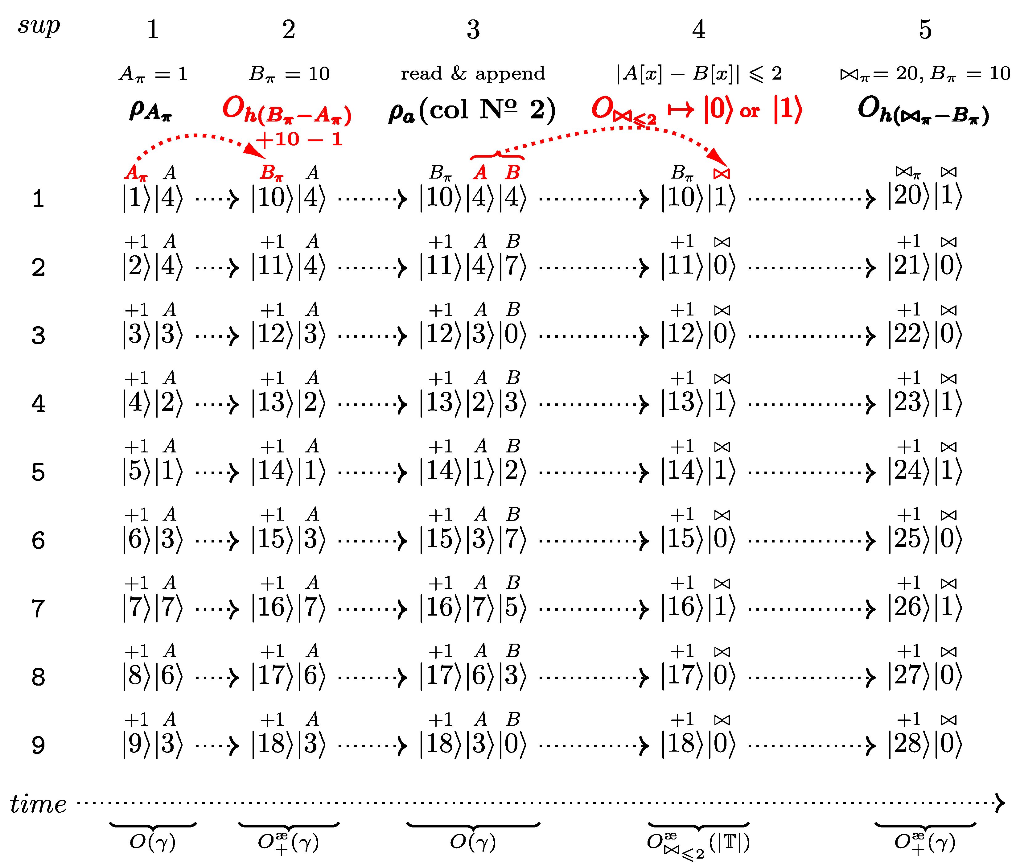
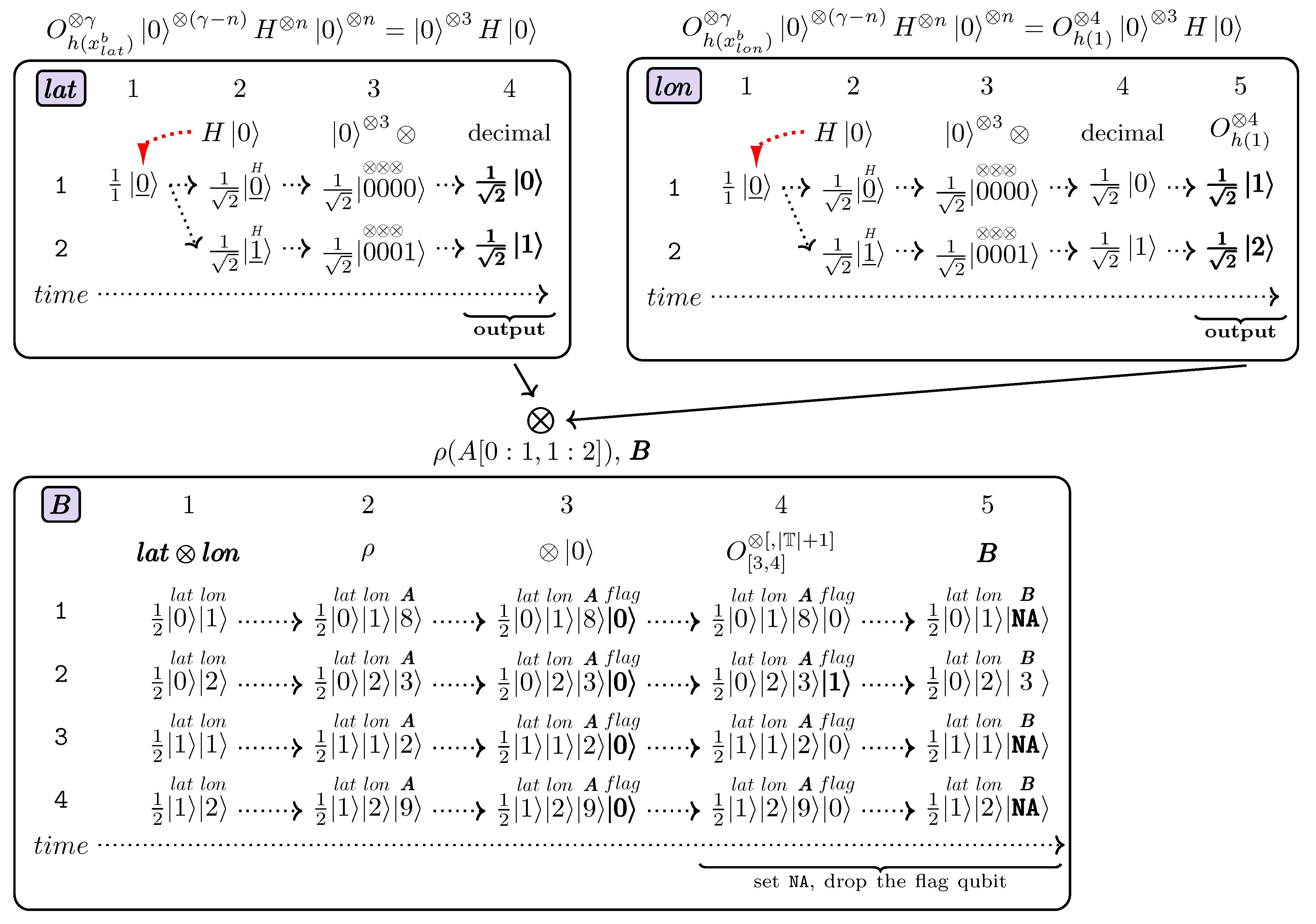
Hyperslabbing frequently occurs as a sub-operation for other array (tensor) operations. Hyperslabbing is a core array (tensor) operation. Hence, let us illustrate it using a QGantt chart to facilitate forming a better intuition. We refer to Figure 9a and hyperslab $A[3,0:3]$ to provide concrete indexes and numbers for a clear description. Suppose that $A_{\pi }=0$ and $\gamma =4$. If we lay out A in a row-wise manner, $x^b=12$. The QGantt chart helps to develop intuition behind the approach and understand the hyperslabbing algorithm, Figure 12.

Figure 12 displays 6 superpositions. We need 4 steps in the presented case to obtain the hyperslab $A[3,0:3]$ (column № 4 just contains a decimal representation of values from column № 3). The resulting hyperslab contains 4 elements, so $n=2$: two qubits are sufficient to carry indexes of the sought cells. Hence, we start from $\left|\underline{00}\right.〉={\left|0\right.〉}^{\otimes 2}$, see $(1,1)$: row (term) № 1 and column (superposition) № 1. Both elements (zero symbols) in $\left|\underline{00}\right.〉$ are underlined because both of them participate in the next operation: they are inputs to the Hadamard operator $H^{\otimes 2}$.

The expression $H^{\otimes 2}{\left|0\right.〉}^{\otimes 2}$ appears in the head of column № 2 to give a hint about how the terms of the superposition in column № 2 were produced. Two red dotted lines with red arrows at their ends point to the qubits that were affected by the Hadamard operator applied to $(1,1)$. All terms in column № 2 were derived from $(1,1)$ as shown by dotted gray lines. Unlike the previous charts (e.g., Figure 5), the lines do not have arrows: the chart in Figure 12 is much larger. Therefore, the dotted line style and the absence of arrows are one of many possible examples of QGantt charts’ flexibility in reducing visual load.

Figure 12. QGantt chart for hyperslabbing $A[3,0:3]$ in Figure 9a.

Figure 12. QGantt chart for hyperslabbing $A[3,0:3]$ in Figure 9a.

All qubits in each term of column № 2 are also underlined to indicate that they were generated as a result of the operation that we have already described (the Hadamard operator $H^{\otimes 2}$). However, underlining is not sufficient in Figure 12 compared to the previous QGantt charts. Therefore, small letters H are placed over each qubit in each term of column № 2. First, to avoid scrolling (it is possible to put H only over the first term, but there can be many of them in a single column). Second, to give a clue that they result from applying the Hadamard operator.

One of the reasons for placing an operator symbol over a qubit of a term in a superposition is to distinguish between different operations and clearly indicate which operation produced which qubit. If only underlining is used, such indications are not possible when multiple or different operations take place. For example, terms in column № 2 were produced by $H^{\otimes 2}$ while terms in column № 3 are the result of the tensor product. A small symbol ⊗ over each of the two leftmost qubits in column № 3 indicates that only these two qubits are new while the remaining two rightmost qubits were copied from the respective terms in column № 2 (inputs and outputs can be tracked using dotted gray lines).

In column № 3 we append the remaining qubits to form a quantum pointer for the $\rho$ operation. In this example, $\gamma =4$ and $\gamma -n=4-2=2$, so we append ${\left|0\right.〉}^{\otimes 2}=\left|00\right.〉$. New qubits are marked with a small ⊗ symbol on top of them.

Column № 4 displays decimal values of the terms in column № 3.

Column № 5 presents the result of applying the oracle $O_{h(A_{\pi }+x^b)}^{\otimes \gamma }=O_{h(0+12)}^{\otimes 4}$ in this example, i.e., adding 12 to each term in column № 4. It is clear that it is possible to implement this oracle even in current quantum machines.

Finally, column № 6 contains the result of reading the hyperslab from QRAM. For the $\rho$ operation, column № 5 serves as a quantum pointer which contains indexes of array cells that we would like to read. As a result, the $\rho$ operation produced a superposition where the index values are entangled with the respective cell values, column № 6. For example, the index of the only NA cell in the example hyperslab is 13, so we have term ${\displaystyle \raisebox{1ex}{$1$}\!\left/ \!\raisebox{-1ex}{$2$}\right.}\left|13\right.〉\left|\mathtt{NA}\right.〉$ in column № 6. Note that $A[3,0:3]=\{1,\mathtt{NA},1,0\}$.

It is straightforward to extend the algorithm for hyperslabbing a higher-dimensional array (tensor) located in QRAM.

4.7. Quantum Array (Tensor) Joins

Array joins are significantly different compared to relational DBMS (RDBMS) joins. They also have subtypes and always enjoy attention similar to RDMBS joins, as an efficient array join is a challenging task [17,59,82]: even specialized array indexing techniques are designed to accelerate array joins [8,82].

Figure 13. The absolute values of sea surface wind speed differences between midnight and 06:00 o’clock UTC+00 of the 28^th of August, 2005 that are greater or equal to 5 m/s.

Figure 13. The absolute values of sea surface wind speed differences between midnight and 06:00 o’clock UTC+00 of the 28^th of August, 2005 that are greater or equal to 5 m/s.

Consider a popular value similarity join which takes two N-d arrays (tensors) $A,B$ and a predicate $\theta$ as input such that $A(d_1,d_2,\dots ,d_N):\mathbb{T}$ and $B(d_1,d_2,\dots ,d_N):\mathbb{T}$. Note that A and B have the same dimensions to be able to perform the join. The join result $C=A{\bowtie }_{\theta }B$ is also an N-d array (tensor) $C(d_1,d_2,\dots ,d_N):\{\mathtt{NA},0,1\}$ whose cell values are defined in Equation (23).

$$C[x_1,x_2,\dots ,x_N]=\left\{\begin{array}{cc}\mathtt{NA},\hfill & \mathrm{if}A[x_1,x_2,\dots ,x_N]=\mathtt{NA}\mathrm{or}B[x_1,x_2,\dots ,x_N]=\mathtt{NA}\hfill \\ 1,\hfill & \mathrm{if}\theta (A[x_1,x_2,\dots ,x_N],B[x_1,x_2,\dots ,x_N])\mathrm{is}\mathrm{true}\hfill \\ 0,\hfill & \mathrm{otherwise}\hfill \end{array}\right.$$

(23)

It is also possible to replace 0 with NA or to introduce additional values when A or B contains NA, e.g., yield 2 if $A[x_1,x_2,\dots ,x_N]=\mathtt{NA}$ and 3 if $B[x_1,x_2,\dots ,x_N]=\mathtt{NA}$.

Array similarity joins appear in Earth data engineering in diverse ways. Consider our illustrative dataset that contains the sea surface wind speed, Section 4.3. Let us take two subsequent 2-d arrays of wind speed for the 28^th of August, 2005 at midnight UTC+00 (Figure 7) and the same day at 06:00 o’clock UTC+00. To mark places on the map where wind speed values have changed over 5 m/s during this 6-h interval, we can perform the value similarity join with $\theta :a,b\mapsto \mathrm{true}\mathrm{if}|a-b|⩾5$, false otherwise. Figure 13 plots the respective differences of values. To get a value similarity join result, substitute all non-NA values by 1 and NA values (gray area) accordingly in Figure 13. Note that the user can tune the wind speed threshold multiple times triggering repeated computations. For example, the user can try 1, 3, 5, 10 m/s and other values to better explore the difference. This tuning use-case scenario can be time-consuming, so the join algorithm must be fast.

Classical Challenge 3. How to efficiently perform array joins?

Let us state the problem using a toy example to track the specific cell values, their indexes, and clearly illustrate the quantum join algorithm. W.l.o.g., consider two 2-d arrays: $A(lat,lon)$ and $B(lat,lon)$, Figure 14a and Figure 14b respectively, such that $\left|lat\right|=\left|lon\right|=3$.

Next, let $\theta :a,b\mapsto \mathrm{true}\mathrm{if}|a-b|⩽2$. The value similarity join $A{\bowtie }_{⩽2}B$ is in Figure 14c. Cells of $A,B$ and $A{\bowtie }_{⩽2}B$ are dashed if they satisfy the predicate. Empty cells in Figure 14c may be equal to 0 or NA.

Figure 14. Illustration of the value similarity join $A{\bowtie }_{⩽2}B$.

Figure 14. Illustration of the value similarity join $A{\bowtie }_{⩽2}B$.

Quantum Look at Challenge 3.

Let us extend $\rho$ to read memory cells addressed only by the first $\gamma$ qubits (cell indexes $\left|j\right.〉$) of ${\pi }_a={\sum }_j{\psi }_j\left|j\right.〉\left|·\right.〉$ and entangle the values with ${\pi }_a$ as well (a kind of read-and-append): ${\rho }_a\left({\pi }_a\right)={\pi }_a\leftarrow {\sum }_j{\psi }_j\left|j\right.〉\left|·\right.〉|D_j\rangle$, Table 1. Note that the value combinations of these qubits will remain unique if we add or subtract a constant to or from the first $\gamma$ qubits. We hope that the hardware community will consider realizing ${\rho }_a$ to boost Array (Tensor) DBMSs and other tensor systems.

Now, with the inherent quantum parallelism

$${\rho }_a\left(O_{h(B_{\pi }-A_{\pi })}^{\otimes [\gamma ,]}{\rho }_{A_{\pi }}\right)={\psi }_x\left|B_{\pi }+x\right.〉\left|A\left[x\right]\right.〉\left|B\left[x\right]\right.〉={\rho }_{A,B}$$

(24)

where $A_{\pi }$ and $B_{\pi }$ are addresses of $A\left[0\right]$ and $B\left[0\right]$ respectively, $A,B$ are laid out in QRAM in a row-wise order similar to Figure 9, ${\rho }_{A_{\pi }}$ is the result of the read operation (all cells of A), and $O_h^{\otimes [\gamma ,]}$ acts only on the first $\gamma$ qubits, Table 1.

Note that this approach is also flexible: if $\rho$ for A omits ${\psi }_j\left|j\right.〉\left|\mathtt{NA}\right.〉$ for some reason, $B\left[j\right]$ will also be skipped. Hence, we do not need an extension where $\rho$ reads addresses from one register and attaches data to another, we can use the same quantum register. We can also optimize the join via reordering (join B with A or A with B) in future work.

Finally,

$$A{\bowtie }_{\theta }B=\omega \left(O_{h({\bowtie }_{\pi }-B_{\pi })}^{\otimes [\gamma ,]}{O}_{\bowtie }^{\otimes [,2|\mathbb{T}\left|\right]}{\rho }_{A,B}\right)$$

(25)

where ${\bowtie }_{\pi }$ is the address of $A{\bowtie }_{⩽2}B$ (the join result) and $O_{\bowtie }^{\otimes [,2|\mathbb{T}\left|\right]}$ acts on the last $2\left|\mathbb{T}\right|$ qubits (pairs of values from A and B), Table 1. Here $O_{\bowtie }$ is defined as follows (it is straightforward to extend $O_{\bowtie }$ to account for NA):

$$O_{\bowtie }:\left\{\begin{array}{cc}\left|A\left[x\right]\right.〉\left|B\left[x\right]\right.〉\mapsto \left|1\right.〉,\hfill & \mathrm{if}\theta \left(A\right[x],B[x\left]\right)\hfill \\ \left|0\right.〉,\hfill & \mathrm{otherwise}\hfill \end{array}\right.$$

(26)

Let us analyze the asymptotic runtime complexity of the quantum array (tensor) join algorithm. We start from preparing the quantum register to perform the read operation which retrieves array A. The preparation takes $O_{+}^{\ae }\left(\gamma \right)$ time. If we further assume the same cost of the arithmetic addition operation similarly to the hyperslabbing, Section 4.6, we can run the preparation in $O\left(\gamma \right)$ time. As agreed, the reading process takes $O\left(\gamma \right)$ time.

Now we have a superposition that contains the elements of A. The next step is to modify this superposition for the read-and-append operation. The asymptotic runtime cost of these modifications is similar to the preparation for reading A: $O_{+}^{\ae }\left(\gamma \right)$, which can be further refined to $O\left(\gamma \right)$, as in the previous preparation step. If read-and-append is of the similar asymptotic complexity to the usual read, we will obtain ${\rho }_{A,B}$ also in $O\left(\gamma \right)$ time.

We are ready to perform the join logic in $O_{{\bowtie }_{⩽2}}^{\ae }\left(\right|\mathbb{T}\left|\right)$ time (two cell values and a constant, each stored in $\left|\mathbb{T}\right|$ qubits, and ancillary qubits). In this specific example, we need to subtract cell values and compare them to a constant in $O_{-}^{\ae }\left(\right|\mathbb{T}\left|\right)+O_{compare}^{\ae }\left(\right|\mathbb{T}\left|\right)$ time (each operation runs on a pair of values, each stored in $\left|\mathbb{T}\right|$ qubits, and ancillary qubits). Again, with contemporary quantum circuits for subtraction and comparison [172,173,174], it is possible to conclude that $O_{-}^{\ae }\left(\right|\mathbb{T}\left|\right)+O_{compare}^{\ae }\left(\right|\mathbb{T}\left|\right)=O\left(\right|\mathbb{T}\left|\right)$.

Figure 15. QGantt chart for creating value similarity join $A{\bowtie }_{⩽2}B$ in Figure 14.

Figure 15. QGantt chart for creating value similarity join $A{\bowtie }_{⩽2}B$ in Figure 14.

Finally, we prepare the quantum superposition for the write operation in $O_{+}^{\ae }\left(\gamma \right)=O\left(\gamma \right)$ time and write the array (tensor) join result into QRAM in $O\left(\gamma \right)$ time. Hence,

$$\begin{array}{cc}\hfill \pounds \left(A{\bowtie }_{\theta }B\right)& =O_{+}^{\ae }\left(\gamma \right)+O\left(\gamma \right)+O_{+}^{\ae }\left(\gamma \right)+O\left(\gamma \right)+\pounds \left(\theta \right)+O_{+}^{\ae }\left(\gamma \right)+O\left(\gamma \right)\hfill \\ \hfill & =O\left(\gamma \right)+O\left(\gamma \right)+O\left(\gamma \right)+O\left(\gamma \right)+\pounds \left(\theta \right)+O\left(\gamma \right)+O\left(\gamma \right)\hfill \\ \hfill & =O\left(\gamma \right)+\pounds \left(\theta \right)\hfill \end{array}$$

(27)

To continue analyzing our example in this subsection, we can additionally specify $\pounds \left(\theta \right)$, as discussed above:

$$\begin{array}{cc}\hfill \pounds \left(A_{{\bowtie }_{⩽2}}B\right)& =O\left(\gamma \right)+\pounds \left(\theta \right)\hfill \\ \hfill & =O\left(\gamma \right)+O_{{\bowtie }_{⩽2}}^{\ae }\left(\right|\mathbb{T}\left|\right)=O\left(\gamma \right)+O_{-}^{\ae }\left(\right|\mathbb{T}\left|\right)+O_{compare}^{\ae }\left(\right|\mathbb{T}\left|\right)\hfill \\ \hfill & =O\left(\gamma \right)+O\left(\right|\mathbb{T}\left|\right)=O(\gamma +|\mathbb{T}\left|\right)\hfill \end{array}$$

(28)

For example, $\gamma =32$ and $\left|\mathbb{T}\right|=8$ (byte). Recall that $log\left|A\right|=log\left|B\right|=n⩽\gamma$, so we obtain an exponential speedup.

The respective QGantt chart for illustrative matrices in Figure 14 is in Figure 15. We have already examined the complexity of $\rho$ and arithmetic operations in previous examples. Therefore, we use decimal instead of binary numbers and do not show all $\gamma$ qubits in the QGantt chart explicitly. We also omit phase (amplitude) values for superposition terms as we do not modify them. We have shown how $\rho$ and hyperslabbing work in Figure 12, so we immediately start from the result of $\rho$ in Figure 15.

Column № 1 shows the result of reading A from QRAM, 9 cell values in total. We assumed that $A_{\pi }=1$, the index of $A\left[0\right]$ in QRAM (this is indicated at the top of column № 1). In other words, column № 1 contains the value of ${\rho }_{A_{\pi }}$ (Equation (24)) as stated at the top of column № 1, below $A_{\pi }=1$. The top row of a QGantt chart is a place where it is possible to place auxiliary information for each column.

Each term in column № 1 consists of 2 parts: the left decimal number is the cell index and the right is the cell value of A for that index. We put a small letter A on top of each cell value to make the semantics of the value clear. It is especially useful when cells of two or more arrays are present in the same superposition term like in column № 3. All indexes of A that were read by $\rho$ are sequential. Hence, $+1$ appears above each index value in column № 1. Finally, the asymptotic complexity of the read operation is $O\left(\gamma \right)$ as indicated under the curly brace for column № 1, below the $time$ axis.

To get the superposition in column № 2, each term in column № 1 undergoes the transformation by the oracle $O_{h(B_{\pi }-A_{\pi })}$, Equation (24). We assume that $B_{\pi }=10$ (see the top of column № 2). The oracle and $+10-1$ annotate the dotted red line with arrow which illustrates the transformation of $(1,1)$ to $(1,2)$: $1+(10-1)=10$. This step prepares for the next read-and-append operation. The asymptotic cost of transforming the superposition in column № 1 to column № 2 is $O_{+}^{\ae }\left(\gamma \right)$, as stated under the curly brace for column № 2, below the $time$ axis.

Note that to add qubits, an oracle $O_{h\left(x\right)}$ needs some ancillary qubits: to store x, intermediate numbers, and other information. The same goes for $O_{{\bowtie }_{⩽2}}$. Note that $O_{\bowtie }^{\otimes [,2|\mathbb{T}\left|\right]}$ in Equation (25) does not account for ancillary qubits and also focuses only on the input cell values stored in $2\left|\mathbb{T}\right|$ qubits. However, it is clear that these oracles rely on standard quantum computing transformations. Therefore, instead of discussing well-known arithmetic implementations that may obscure the main ideas behind array operations, we concentrate on the Array (Tensor) DBMS algorithms.

Column № 3 plots the result of the ${\rho }_a$ operation (read-and-append), completing the first step of the join operation, Equation (24). The asymptotic complexity appears below the $time$ axis and is the same as for the $\rho$ operation. The last two parts of each term in column № 3 contain cell values of arrays A and B. Small letters A and B are placed above respective cell values in each term of column № 3 to facilitate visual matching of values with the array from which they were retrieved. The first part of each term in column № 3 is equal to the cell value index in QRAM for array B. Now we are ready to perform the join.

Column № 4 contains the result of applying $O_{{\bowtie }_{⩽2}}$ to the superposition in column № 3, Equation (25). The dotted red line with arrow shows the transformation of $(1,3)$ to $(1,4)$.

Finally, column № 5 is the superposition prepared to be written to QRAM by $\omega$, Equation (25). We assume that ${\bowtie }_{\pi }=20$, see the top of column № 5. The oracle and its asymptotic complexity are similar to that in column № 2. After $\omega$, the array that represents the join result will appear in QRAM in the row-wise layout starting from index 20.

4.8. Quantum Array Algebra

Array (Map) Algebra is widely used in the industry and constitutes a large portion of Array (Tensor) DBMS workloads  [7,8].

A typical expression that is a representative map algebra query is a popular vegetation index NDVI = (nir − r)/(nir + r) that accepts nir and r: 2-d arrays, intensities of reflected solar radiation in the near-infrared and visible red spectra respectively.

Map algebra is an excellent candidate for unprecedented speedups, as many of its queries represent algebraic expressions amenable to automatic translations to quantum circuits, unlike arbitrary classical functions. A flexible Earth data engineering tool like a Quantum Array (Tensor) DBMS can be especially useful for map algebra operations on data that appears to be already in QRAM or RAQM.

Classical Challenge 4. How to efficiently execute queries that contain array (map) algebra expressions?

Although it is relatively straightforward to compute ndvi, there is a class of functions like $f(\alpha ,·)$ with a user-tunable parameter $\alpha$ adjusted by users interactively. Dozens of such functions exist [12], e.g., savi, pvi and others, Figure 16. The user can tune $\alpha$, e.g., ${\alpha }_{new}={\alpha }_{old}+\Delta \alpha$, to experimentally find appropriate $f(\alpha ,·)$ values for an area of interest. Sophisticated approaches to compute $f(\alpha +\Delta \alpha ,·)$ exist [12], but quantum computing may offer an exponential speedup.

Users tend to spend vast amounts of time for Interactive Data Science, but can experience increased response times in tune-recompute scenarios. As a user typically spends their time waiting for query results in front of a computer, each successive data processing delay, even within a split second, increases human fatigue and thereby reduces the quality of work and understanding of the data.

Quantum Look at Challenge 4. The approach of executing map algebra queries is similar to the array join approach presented in Section 4.7.

$O_m^{\otimes [,k|\mathbb{T}\left|\right]}{\rho }_{A_1,A_2,\dots ,A_k}$ applies a local map algebra operation m to k arrays $A_1,A_2,\dots ,A_k$ in a single superposition ${\rho }_{A_1,A_2,\dots ,A_k}$ prepared in a similar way as for the join operation, see column № 3 in Figure 15.

A typical asymptotic cost for a Quantum Array (Tensor) DBMS to execute ndvi and other frequent array algebra expressions is expected to be just $O_{\mathrm{arithmetic}}^{\ae }\left(\right|\mathbb{T}\left|\right)$. Of course, reading, writing, and other accompanying costs exist as for $\pounds \left(A{\bowtie }_{\theta }B\right)$, Equation (27), but in total they are asymptotically exponentially faster than the respective classical costs.

In the case of tunable functions, a naive quantum approach to recompute a function from scratch would still be exponentially faster. Current quantum machines can keep a superposition just for a very small amount of time before decoherence. However, even repetitive $\rho$ and $\omega$ operations that require just $O\left(\gamma \right)$ may be faster compared to classical approaches. Of course, more advanced quantum approaches can also be devised.

4.9. Quantum Array (Tensor) Indexes

Consider again Figure 7 and Figure 8. Suppose it is required to select all CO₂ or wind map cells whose values are within the given range. This is a value-based query. For example, select array cells with mole fraction of CO₂ in the range $[3.77\times {10}^{-4},3.84\times {10}^{-4}]$. If a restriction is applied only to the geographical area, the query is called dimension-based (similar to hyperslabbing, Section 4.6). A single query can combine both types of restrictions. For example, select array cells in the Pacific Ocean (the restriction on $lat$ and $lon$ dimensions) whose wind speed is above 5 m/s (additional restriction on cell values).

To efficiently answer such Earth data engineering queries without scanning all array cells for each query, array (tensor) indexes are built beforehand. Once a query arrives, an array (tensor) index is used to accelerate query answering. Unlike RDBMS indexes, Array (Tensor) DBMS indexes can be used alone, without original data. They reorganize arrays to reduce I/O compared to querying original data [12,16,79,82,175].

Classical Challenge 5. How to efficiently perform dimension- and value-based array (tensor) operations, often within a single query?

Let us take a tiny matrix A as a running example for this subsection and define it as $A(lat,lon):\mathbb{T}=\left\{\right\{5,8,3\},\{3,2,9\},\{1,7,4\left\}\right\}$, where $lat\langle 3\rangle :\mathbb{T}=\{0,1,2\}$ and $lon\langle 3\rangle :\mathbb{T}=\{0,1,2\}$ (we use $\mathbb{T}$ both for values and indexes for simplicity).

The following query is both dimension- and value-based, because it extracts a subarray B that will contain values from A that are within the (1) value range $[3,4]$ and (2) index ranges $[0,1]$ and $[1,2]$ for the first and second axes, respectively:

SELECT $B⊑A$

WHERE A.value IN $[\mathbf{3},\mathbf{4}]$AND

              A.$lat$ IN $[\mathbf{0},\mathbf{1}]$ AND

              A.$lon$ IN $[\mathbf{1},\mathbf{2}]$

Figure 17 illustrates the query challenges. The same array A is depicted in Figure 17a–c.  In all figures, the sought area $A[0:1,1:2]$ is surrounded by blue dotted lines, while the respective indexes on the $lat$ and $lon$ axes are inside the dashed red areas. Figure 17a additionally dashes cells with red lines in the whole array A that are within the specified range of $[3,4]$, but not necessarily within the specified area. Figure 17b dashes cells with similar lines that are only within the specified area, but not the given cell value range. Finally, Figure 17c marks only the single cell with dashed lines that satisfies all query criteria and is the query result.

The challenge is to avoid scanning the whole array and even the area that satisfies the given dimension range (geographical area). Array A is tiny, but even in this case it is clear that the resulting cell $A[0,3]$ constitutes only 25% of the hyperslab $A[0:1,1:2]$: the query is very selective. Without specialized indexing techniques, the problem becomes much worth for bigger arrays, for queries with loose dimension constraints or for highly selective queries when it is required to scan a large portion of an array or the whole array in order to answer the query.

Quantum Look at Challenge 5.

If array A is in QRAM, indexing is optional. Further, if A is not readonly, maintaining an index would be much more efficient using RAQM instead of QRAM (A itself can still be in QRAM). If A is readonly and we expect a sufficiently large number of queries to A that will compensate for the index preparation time, we may resort to QRAM to keep an index.

To answer the query in $O(log|A\left|\right)+O_{\mathrm{arithmetic}}^{\ae }(\gamma +|\mathbb{T}\left|\right)$, we may not use an index. First, let us see how we can answer the query without any index, but using quantum memory and inherent quantum parallelism.

We can split the query into two steps: (1) hyperslabbing and (2) value selection. That is, in step № 1, extract $A[0:1,1:2]$ using the technique proposed earlier, Section 4.6. We need to cover the value selection step in this subsection, i.e., seek cells whose values are within the range $[3,4]$ and whose coordinates are in $A[0:1,1:2]$. Suppose that the value range (the value-based part of the query) is given as $[v^b,v^e]$, where $v^b,v^e\in \mathbb{T}$.

We propose two approaches for executing step № 2. The first approach, the equality approach, assumes that we cannot use a range comparison oracle $O_{[v^b,v^e]}^{\otimes [,|\mathbb{T}|+1]}$ (Equation (29)), but rather an equality test oracle $O_{=}^{\otimes [,2\times |\mathbb{T}|+1]}$ at step № 2. The second approach, the range approach, uses oracle $O_{[v^b,v^e]}^{\otimes [,|\mathbb{T}|+1]}$ (Equation (30)) at step № 2. For example, oracle $O_{[v^b,v^e]}^{\otimes [,|\mathbb{T}|+1]}$ may not be available, can be costlier than oracle $O_{=}^{\otimes [,2\times |\mathbb{T}|+1]}$, or we cannot use oracle $O_{[v^b,v^e]}^{\otimes [,|\mathbb{T}|+1]}$ for some other reasons.

We define the oracles as follows. Oracle $O_{=}^{\otimes [,2\times |\mathbb{T}|+1]}$ operates on a pair of values and one ancillary qubit (flag) to store the result (we also need some ancillary qubits to perform the equality test, but we do not show them as such test is a standard operation):

$$O_{=}^{\otimes [,2\times |\mathbb{T}|+1]}:u,v\mapsto \left\{\begin{array}{cc}\left|1\right.〉,\hfill & \mathrm{if}u=v\hfill \\ \left|0\right.〉,\hfill & \mathrm{otherwise}\hfill \end{array}\right.$$

(29)

Oracle $O_{[v^b,v^e]}^{\otimes [,|\mathbb{T}|+1]}$ operates on one value and one ancillary qubit (flag) to store the result, Equation (30). We also need ancillary qubits to perform the test-in-range or the comparison of a with $v^e$ and $v^b$. The number of such qubits depends on the algorithm used, but in general this number and the respective circuit depth can be larger than for $O_{=}^{\otimes [,2\times |\mathbb{T}|+1]}$. For example, we can implement the comparison of two values by subtracting one value from another and checking the sign of the result.

$$O_{[v^b,v^e]}^{\otimes [,|\mathbb{T}|+1]}:a\mapsto \left\{\begin{array}{cc}\left|1\right.〉,\hfill & \mathrm{if}a\in [v^b,v^e]\hfill \\ \left|0\right.〉,\hfill & \mathrm{otherwise}\hfill \end{array}\right.$$

(30)

The equality approach not only shows how to answer both a dimension- and value-based query, but also presents how multistage quantum algorithms can look like and how to illustrate them step-by-step using a special type of quantum diagram, Section 5.2. In addition, the equality approach uncovers interesting cases where it is desirable to have NA in cell indexes and presents possible actions in such cases when there is no respective hardware support, Section 4.4.2. Importantly, other array quantum algorithms, not only related to quantum indexing, can also arrive at similar situations as described in our equality approach. Therefore, the equality approach is also useful from a broader perspective.

Let us first describe the equality approach. Further assume that $v^e-v^b+1=2^n$ and $\left|\mathbb{T}\right|\ge n$. Otherwise, we will need to perform additional comparison operations to filter out irrelevant cell values. First, recall that we would like to avoid comparisons. Second, we aim to showcase the main ideas of the approach and prevent obscuring the algorithm. Anyway, if $v^e-v^b+1=2^n$, systems may optimize by using the presented algorithm to avoid additional operations and possibly reduce the runtime. Next, suppose that $B^{\prime }=A[0:1,1:2]$ (or some other hyperslab). The first step prepares for the direct $1:1$ equality test (not a generic test-in-range with $O_{[v^b,v^e]}^{\otimes [,|\mathbb{T}|+1]}$ which is more expensive):

$$B_1=B^{\prime }\otimes \left(O_{h\left(v^b\right)}^{\otimes \left|\mathbb{T}\right|}{\left|0\right.〉}^{\left(\right|\mathbb{T}|-n)}{H}^{\otimes n}{\left|0\right.〉}^{\otimes n}\right)$$

(31)

where $O_h$ is an oracle for the standard addition as in Equation (21). Now, each element of array $B^{\prime }$ is replicated $2^n$ times and co-located with each integer value within the range $[v^b,v^e]$. It is possible to perform the equality test as follows: for each pair of values from $B^{\prime }$ and $[v^b,v^e]$ we check if they are equal or not. In classical computing this is equivalent to two nested loops:

for each value $b[x_1,x_2]\in B^{\prime }$

     for each value $q\in [v^b,v^e]$

        if $b[x_1,x_2]=q$ then add $b[x_1,x_2]$ to the result

The code above performs an exhaustive search, which is the worst and least efficient technique for classical, but not quantum computing. On the contrary, quantum computing can execute the same search just in a constant amount of time.

The next step is to perform the direct 1:1 equality test and save the result in an ancillary qubit:

$$B_2=O_{=}^{\otimes [,2\times |\mathbb{T}|+1]}\left(B_1\otimes \left|0\right.〉\right)$$

(32)

where $O_{=}^{\otimes [,2\times |\mathbb{T}|+1]}$ is our equality oracle, Equation (29).

Finally, using the equality test result, we assign NA to indexes and values where the flag qubit equals $\left|0\right.〉$. $B_2$ can have the same shape as $A[0:1,1:2]$, yielding the final result with a copy of $A[0,2]$:

$$B(la{t}_B,lo{n}_B):\mathbb{T}=\{\{\mathtt{NA},3\},\{\mathtt{NA},\mathtt{NA}\}\}$$

(33)

where $la{t}_B\langle 2\rangle :\mathbb{T}=\{0,1\}$ and $lo{n}_B\langle 2\rangle :\mathbb{T}=\{1,2\}$. We elaborate on why we set NA not only to values, but also to indexes in Section 5, where we also present post-processing steps to get Equation (33). After this final step we have several options. First, just write the result into QRAM. Second, write the result into RAQM. Last, use the result in subsequent quantum algorithms. In the last two options, we also may perform NA elimination, Section 4.5.4.

Now, let us describe the second approach, the range approach, if oracle $O_{[v^b,v^e]}^{\otimes [,|\mathbb{T}|+1]}$ is allowed. It can be formulated more concisely, Equation (34):

$$B_1=O_{[v^b,v^e]}^{\otimes [,|\mathbb{T}|+1]}\left(B^{\prime }\otimes \left|0\right.〉\right)$$

(34)

To get B, we need to post-process $B_1$: assign NA to cell values where the flag is $\left|0\right.〉$.

A detailed, step-by-step example of efficiently executing the query on page 31 which is both dimension- and value-based is in Section 5.

The asymptotic complexity analysis reveals the following runtime cost of the proposed algorithm that is plugged with the equality approach. First, we hyperslab array A in $O({\gamma }^2+\gamma )$ time. The runtime differs from hyperslabbing a 1-d array, Section 4.6, because we need to convert the wide strip layout to the narrow layout, which requires multiplication that can run in quadratic time depending on the number of qubits in the input operands [172,173,174]. The cost can be reduced to $O\left(\gamma \right)$ if we keep A in the narrow layout.

Next, we prepare for the 1:1 direct equality test. First, we apply the Hadamard operator in $O\left(n\right)=O\left(\right|\mathbb{T}\left|\right)$ time. Second, we run the oracle in $O_{+}^{\ae }\left(\right|\mathbb{T}\left|\right)=O\left(\right|\mathbb{T}\left|\right)$ time. Finally, we need to entangle the hyperslab with the prepared values. However, we assume the cost of this step to be $O\left(1\right)$, because we can allocate the required number of qubits in a quantum register beforehand to avoid additional entanglement operations.

We are ready to perform the direct 1:1 equality test in $O_{=}^{\ae }\left(\right|\mathbb{T}\left|\right)=O\left(\right|\mathbb{T}\left|\right)$ time. Afterwards, we assign NA to respective indexes and values in $O\left(\right|\mathbb{T}|+\gamma )$ time. Therefore,

$$\begin{array}{c}\hfill \pounds \left(\mathrm{dimension}\text{-}\mathrm{and}\mathrm{value}\text{-}\mathrm{based}\mathrm{query}:2\text{-}\mathrm{d}\mathrm{array},\mathrm{wide}\mathrm{layout}\right)=\\ \hfill O({\gamma }^2+\gamma )+O\left(n\right)+O_{+}^{\ae }\left(\right|\mathbb{T}\left|\right)+O_{=}^{\ae }\left(\right|\mathbb{T}\left|\right)+O\left(\right|\mathbb{T}|+\gamma )\\ \hfill =O({\gamma }^2+\gamma )+O\left(\right|\mathbb{T}\left|\right)+O\left(\right|\mathbb{T}\left|\right)+O\left(\right|\mathbb{T}\left|\right)+O\left(\right|\mathbb{T}|+\gamma )\\ \hfill =O({\gamma }^2+\gamma )+O\left(\right|\mathbb{T}\left|\right)+O\left(\right|\mathbb{T}|+\gamma )\\ \hfill =O({\gamma }^2+\gamma +|\mathbb{T}\left|\right)\end{array}$$

(35)

Further alternative post-processing steps are described in Section 5.2.

Unlike the classical algorithm without any indexes, the presented quantum algorithm efficiently answers the query: $O({\gamma }^2+\gamma +|\mathbb{T}\left|\right)$ for a 2-d array with up to $2^{\gamma }$ elements instead of classical $O\left(2^{\gamma }\right)$, yielding an exponential speed.

The asymptotic cost for the algorithm that utilizes the range approach is also $O({\gamma }^2+\gamma +|\mathbb{T}\left|\right)$, if oracle $O_{[v^b,v^e]}^{\otimes [,|\mathbb{T}|+1]}$ is implemented using subroutines not costlier than $O_{-}^{\ae }\left(\right|\mathbb{T}\left|\right)$.

We can improve further by building indexes for an array (tensor) beforehand. Multiple reasons can exist for this. For example, it may be beneficially to split an array (tensor) into multiple parts that require less qubits for storage, and, thus, less time for I/O.

Following the classical array (tensor) indexing approach [8], we can create separate indexes for value ranges $1..3$, $4..6$, and $7..9$:

$${\mathcal{L}}_{1,3}\langle 3,3\rangle ={\psi }_1\left|2\right.〉\left|0\right.〉\left|1\right.〉+{\psi }_2\left|1\right.〉\left|1\right.〉\left|2\right.〉+{\psi }_3\left|0\right.〉\left|2\right.〉\left|3\right.〉$$

(36)

${\mathcal{L}}_{4,6}$ and ${\mathcal{L}}_{7,9}$ are similar to ${\mathcal{L}}_{1,3}$. Equation (36) shows a wide quantum strip. We apply the same algorithm with the same parameters as above to dimensions and values of ${\mathcal{L}}_{1,3}$ and ${\mathcal{L}}_{4,6}$ (without ${\mathcal{L}}_{7,9}$; its exclusion may yield potential time savings) and then just write each result separately to quantum memory.

However, building and maintaining separate indexes can be costly. To build an index ${\mathcal{L}}_{v^b,v^e}$, we need to tackle superposition terms with NA values (Section 4.5.4). In addition, if QRAM is used, we must alter cell indexes in ${\mathcal{L}}_{v^b,v^e}$ such that ${\mathcal{L}}_{v^b,v^e}$ takes less space in QRAM compared to the original array (tensor), i.e., devise a special array layout. If RAQM is available, it would be excellent to keep ${\mathcal{L}}_{v^b,v^e}$ in a single RAQM cell. A quantum indexing technique must be faster than $O(\gamma +|\mathbb{T}\left|\right)$ to be efficient in terms of asymptotic performance. Another goal of quantum indexing may be to reduce I/O load or other characteristics. We should revisit the question when more information about quantum memory is available.

5. Quantum Network Diagrams (QND)

How to clearly, step-by-step illustrate answering the query from Section 4.9, page 31? It is challenging for a single QGantt chart to accomplish this task. In this section, in addition to QGantt charts, we propose another new type of charts: Quantum Network Diagrams.

5.1. Quantum Network Diagrams: A Bird’s-Eye View

A Quantum Network Diagram consists of several independent QGantt charts that form a DAG (Directed Acyclic Graph). The outputs of several QGantt charts can be entangled and serve as inputs to other QGantt charts in the Quantum Network Diagram. The output/input data dependencies are denoted by arrows. Quantum Network Diagrams can clearly illustrate multistage quantum computations, data flows, and their inter-dependencies in a static manner similar to QGantt charts. Therefore, Quantum Network Diagrams possess virtues similar to QGantt charts, Section 3.

Let us create a Quantum Network Diagram to clearly illustrate the ideas behind the indexing approach in Section 4.9, using our sample query from page 31. In this query, $[v^b,v^e]=[3,4]$, $4-3+1=2$ ($n=1$) and $\left|\mathbb{T}\right|=4$. Hence, we can rewrite Equation (31) as

$$B_1=A[0:1,1:2]\otimes \left(O_{h\left(3\right)}^{\otimes 4}{\left|0\right.〉}^{(4-1)}{H}^{\otimes 1}{\left|0\right.〉}^{\otimes 1}\right)$$

(37)

To extract the hyperslab $A[0:1,1:2]=A[x_{lat}^b:x_{lat}^e,x_{lon}^b:x_{lon}^e]$, let us further assume that $\gamma =4$, $A_{\pi }=0$, $x_{lat}^b=0$, $x_{lat}^e=1$ $x_{lon}^b=1$, $x_{lon}^e=2$. We also assume that $\rho$ reads a wide strip (as we have already noted, it is straightforward to convert a wide strip to its narrow representation and vice versa). Now, complementing Equation (37) with hyperslabbing (see Equation (21)), we obtain

$$\begin{array}{cc}\hfill B_1=\rho & \left[\left(O_{h(0+0)}^{\otimes 4}{\left|0\right.〉}^{(4-1)}{H}^{\otimes 1}{\left|0\right.〉}^{\otimes 1}\right)\otimes \left(O_{h(0+1)}^{\otimes 4}{\left|0\right.〉}^{(4-1)}{H}^{\otimes 1}{\left|0\right.〉}^{\otimes 1}\right)\right]\hfill \\ \hfill & \otimes \left(O_{h\left(3\right)}^{\otimes 4}{\left|0\right.〉}^{(4-1)}{H}^{\otimes 1}{\left|0\right.〉}^{\otimes 1}\right)\hfill \end{array}$$

(38)

Equation (38) can be simplified to

$$B_1=\underset{\rho }{\underbrace{\rho \left[\underset{lat}{\underbrace{\left({\left|0\right.〉}^{\otimes 3}H\left|0\right.〉\right)}}\otimes \underset{lon}{\underbrace{\left(O_{h\left(1\right)}^{\otimes 4}{\left|0\right.〉}^{\otimes 3}H\left|0\right.〉\right)}}\right]}}\otimes \underset{val}{\underbrace{\left(O_{h\left(3\right)}^{\otimes 4}{\left|0\right.〉}^{\otimes 3}H\left|0\right.〉\right)}}$$

(39)

To clearly, step-by-step, illustrate Equation (39), we can integrate several QGantt charts into a single Quantum Network Diagram, Figure 18. Let us first describe the Quantum Network Diagram from a bird’s-eye view. The Quantum Network Diagram consists of 5 QGantt charts connected by arrows that represent input/output quantum superpositions. Recall that the quantum indexing algorithm consists of several parts which yield $B_1$, $B_2$, and the resulting array (tensor) B, Section 4.9. We marked logical portions of Equation (39) as $lat$, $lon$, $\rho$, and $val$ for forming latitude, longitude indexes, and the values in the requested value range respectively. It is possible to find respective QGantt charts for computing $lat$, $lon$, $\rho$, $val$, $B_1$, $B_2$, and B in Figure 18. The diagram consumes almost the whole page, but makes it immediately clear what is happening.

Compared to the QGantt charts that we presented earlier in this article, QGantt charts in Figure 18 have additional visual components and formatting, summarized below.

• Each QGantt chart in a Quantum Network Diagram is surrounded with a rectangle to clearly distinguish and visually separate its contents from other QGantt charts that belong to the same Quantum Network Diagram.
• In Quantum Network Diagrams, each QGantt chart has its name (can also be called tag or label) located in the top left corner of each QGantt chart. In Figure 18, QGantt chart names are in bold italic font, placed inside a filled rectangle to better emphasize the names visually, for example,
• QGantt charts can have annotating formulas associated with a whole chart to explain what a QGantt chart aims to produce as its output. A chart annotating formula describes its QGantt chart as a whole in addition to short formulas that can mark superpositions inside a QGantt chart. In Figure 18, such chart annotating formulas are located above QGantt charts and resemble figure captions.
• Symbol ⊗ appears above annotating formulas for QGantt charts which take superpositions as inputs. In Figure 18, the symbol ⊗ appears at the very top of and , because the chronological order of QGantt charts (the order in which their output superpositions must be generated) coincides with their vertical order, from top to bottom. Of course, the symbol ⊗ can appear at any other side of a QGantt chart if the charts are laid out in a different way. We laid out ⊗ above the annotating formula for to indicate that the the output superpositions of and are used in the $\rho$ operation. Similarly, ⊗ appears exactly above $B_1$ in , not $B_2$ or B, to show that the tensor product of outputs of and forms $B_1$—the output of the first stage of the algorithm, Section 4.9.
• Finally, arrows output$\mapsto \otimes$ connect QGantt charts in a DAG (Directed Acyclic Graph). Typically, the last column of a QGantt chart is its output superposition. We additionally mark each such column in , , , and by a curly brace at the bottom of the last column (superposition) with caption “output”. Each arrow that connects QGantt charts starts near this curly brace or its caption. The arrows point to the symbol ⊗ indicating that the superpositions at the beginning of the arrows participate in the tensor product operation. For example, the superposition № 1 in represents the tensor products of and outputs, so the column № 1 is marked as $\mathit{lat}\otimes \mathit{lon}$. Similarly, the first column (superposition) of equals to ${\mathit{B}}_{\mathbf{1}}=\rho \otimes \mathit{val}$, which is the tensor product of outputs of and .

Note that in addition to Equation (39), the Quantum Network Diagram in Figure 18 also contains the QGantt chart named that completes the illustration of the execution of the algorithm from Figure 18 by providing step-by-step actions that lead to getting the dimension- and value-based query result B.

5.2. Efficiently Answering Dimension- and Value-Based Queries Step-by-Step

Now let us describe the logic behind the Quantum Network Diagram in Figure 18. In our example, we execute both a dimension- and value-based query. First, we hyperslab $A[0:1,1:2]$. Therefore, we prepare the superposition of indexes for the $lat$ and $lon$ dimensions in QGantt charts and respectively, in accordance with the algorithm in Section 4.6. As the hyperslabbing algorithm has been already discussed in Section 4.6, we omit the desciption of and which is similar to Figure 12. Therefore, the reader can refer to the description of Figure 12 to understand and .

Figure 18. Quantum Network Diagram for Equation (39).

Figure 18. Quantum Network Diagram for Equation (39).

The only peculiarity of is that it does not require an addition oracle as its output index range starts from 0, representing a special case.

Next, the index ranges of and come to the QGantt chart named which illustrates reading the hyperslab of A, namely $A[0:1,1:2]$, from QRAM. For more clarity, we show a wide quantum strip for $A[0:1,1:2]$ instead of its narrow version. Recall that it is straightforward to switch between wide and narrow strip layouts. The QGantt chart completes the execution of the dimension-based portion of the query.

According to the algorithm in Figure 18, the next step is to prepare the superposition of all values in the range that was submitted as part of the value-based portion of the query. The QGantt chart performs this step in accordance with Equations (31) and (39). Recall that the idea is to perform an exhaustive, direct 1:1 equality test of each value in the hyperslab $A[0:1,1:2]$ with each value within the queried range $[v^b,v^e]=[3,4]$. This is the worst case for classical computing, but it can be executed in asymptotically constant time on a quantum machine.

Now we can compare each value marked by the symbol A in each term of superposition № 2 of with each value of superposition № 5 of . To accomplish this, we form superposition № 1 called $B_1$ in based on the outputs of and . For the sake of clarity, each value in each term of superposition № 1 in is marked by the symbols $lat$, $lon$, A, and $val$ which indicate that the marked values represent $lat$ and $lon$ indexes, the cell values of the hyperslab $A[0:1,1:2]$, and the generated values by within the submitted cell value range $[v^b,v^e]=[3,4]$ respectively. $A[0:1,1:2]$ has 4 values while the range $[v^b,v^e]=[3,4]$ has 2 values. We compare each value of $A[0:1,1:2]$ with each value in the range $[v^b,v^e]=[3,4]$, so we get 8 terms in superposition $B_1$, column № 1 of .

To perform the equality test, we need an additional qubit to store the test result, we call it a flag qubit. Column № 2 in displays the superposition after appending the flag qubit. Initially it is set to $\left|0\right.〉$. The flag qubit is marked by the word flag and appears in bold in column № 2 to show that this qubit is new compared to the previous superposition in column № 1, QGantt chart .

Column № 3 of displays the resulting superposition after applying the equality test oracle. The oracle acts on the values marked by A and $val$, saving the equality test result to the flag qubit; in total on $2\times \left|\mathbb{T}\right|+1$ qubits, excluding possible ancillary qubits. It turns out, that now only term $(3,3)$ has the flag qubit equal to $\left|1\right.〉$. The flag qubit in term $(3,3)$ is bold and underlined to visually indicate that it is different compared to its previous state in term $(3,2)$. Flag qubits in other terms remain equal to $\left|0\right.〉$ and, thus, appear in usual font style in column № 3.

We found only one value that satisfies our dimension- and value-based query: $A[0,2]$, Figure 17c. The next step is to cleanup the superposition in column № 3 to get B, the resulting array (tensor) consisting of only 1 non-NA cell, Equation (33). Ideally, we must remove all terms № 1, 2, 4–8, excluding term № 3. However, recall that it is a non-trivial task in quantum computing, Section 4.5.4.

At a glance, it might seem that we could avoid removing (deleting) terms that do not satisfy the value-based part of the query by just setting NA to cell values. For example, ${\displaystyle \frac{1}{\sqrt{8}}}\stackrel{lat}{\left|0\right.〉}\stackrel{lon}{\left|1\right.〉}\stackrel{\mathit{A}}{\left|8\right.〉}\stackrel{\mathit{val}}{\left|3\right.〉}\left|0\right.〉$ could be easily transformed to ${\displaystyle \frac{1}{\sqrt{8}}}\stackrel{lat}{\left|0\right.〉}\stackrel{lon}{\left|1\right.〉}\stackrel{\mathit{B}}{\left|\mathtt{NA}\right.〉}$ by replacing cell value with NA and dropping the ancillary qubits (notice the letter B over the NA value that indicates that the cell value in the term belongs to the final result). Afterwards, we would just write the resulting superposition into QRAM and get B, Equation (33). However, notice that we have two copies of $A[0,2]$: ${\displaystyle \frac{1}{\sqrt{8}}}\stackrel{lat}{\left|0\right.〉}\stackrel{lon}{\left|2\right.〉}\stackrel{\mathit{A}}{\left|3\right.〉}\stackrel{\mathit{val}}{\left|3\right.〉}\left|\underline{\mathbf{1}}\right.〉$ and ${\displaystyle \frac{1}{\sqrt{8}}}\stackrel{lat}{\left|0\right.〉}\stackrel{lon}{\left|2\right.〉}\stackrel{\mathit{A}}{\left|3\right.〉}\stackrel{\mathit{val}}{\left|4\right.〉}\left|0\right.〉$; the former copy satisfies the query while the latter does not. If we transform ${\displaystyle \frac{1}{\sqrt{8}}}\stackrel{lat}{\left|0\right.〉}\stackrel{lon}{\left|2\right.〉}\stackrel{\mathit{A}}{\left|3\right.〉}\stackrel{\mathit{val}}{\left|4\right.〉}\left|0\right.〉$ to ${\displaystyle \frac{1}{\sqrt{8}}}\stackrel{lat}{\left|0\right.〉}\stackrel{lon}{\left|2\right.〉}\stackrel{\mathit{B}}{\left|\mathtt{NA}\right.〉}$, we will have 2 terms with the same indexes, but different cell values: ${\displaystyle \frac{1}{\sqrt{8}}}\stackrel{lat}{\left|0\right.〉}\stackrel{lon}{\left|2\right.〉}\stackrel{\mathit{B}}{\left|3\right.〉}$ and ${\displaystyle \frac{1}{\sqrt{8}}}\stackrel{lat}{\left|0\right.〉}\stackrel{lon}{\left|2\right.〉}\stackrel{\mathit{B}}{\left|\mathtt{NA}\right.〉}$. An oracle analyzing ${\displaystyle \frac{1}{\sqrt{8}}}\stackrel{lat}{\left|0\right.〉}\stackrel{lon}{\left|2\right.〉}\stackrel{\mathit{A}}{\left|3\right.〉}\stackrel{\mathit{val}}{\left|4\right.〉}\left|0\right.〉$ cannot check whether $A[0,2]$ belongs to the result. We also do not know the number of resulting NA or non-NA cells beforehand, and quantum counting is a too costly operation in this case.

If there is hardware support for NA in cell indexes, as suggested in Section 4.4.2, a possible way would be to transform ${\displaystyle \frac{1}{\sqrt{8}}}\stackrel{lat}{\left|0\right.〉}\stackrel{lon}{\left|2\right.〉}\stackrel{\mathit{A}}{\left|3\right.〉}\stackrel{\mathit{val}}{\left|4\right.〉}\left|0\right.〉$ to ${\displaystyle \frac{1}{\sqrt{8}}}\stackrel{lat}{\left|\mathtt{NA}\right.〉}\stackrel{lon}{\left|\mathtt{NA}\right.〉}\stackrel{\mathit{B}}{\left|3\right.〉}$ and simply avoid writing ${\displaystyle \frac{1}{\sqrt{8}}}\stackrel{lat}{\left|\mathtt{NA}\right.〉}\stackrel{lon}{\left|\mathtt{NA}\right.〉}\stackrel{\mathit{B}}{\left|3\right.〉}$ to QRAM. Let us describe an approach that does not require hardware support of NA in cell indexes.

Column № 4 of contains terms whose cell indexes and values are set to $\left|\mathtt{NA}\right.〉$ if the qubit flag equals $\left|0\right.〉$, Figure 18. All terms where the flag qubit is $\left|0\right.〉$ will collapse to ${\displaystyle \frac{\sqrt{7}}{\sqrt{8}}}\stackrel{lat}{\left|\mathtt{NA}\right.〉}\stackrel{lon}{\left|\mathtt{NA}\right.〉}\stackrel{\mathit{A}}{\left|\mathtt{NA}\right.〉}\stackrel{\mathit{val}}{\left|\mathtt{NA}\right.〉}\left|0\right.〉$. If we drop the ancillary qubits and the flag qubit, we will obtain ${\displaystyle \frac{\sqrt{7}}{\sqrt{8}}}\stackrel{lat}{\left|\mathtt{NA}\right.〉}\stackrel{lon}{\left|\mathtt{NA}\right.〉}\stackrel{\mathit{B}}{\left|\mathtt{NA}\right.〉}$ and ${\displaystyle \frac{1}{\sqrt{8}}}\stackrel{lat}{\left|0\right.〉}\stackrel{lon}{\left|2\right.〉}\stackrel{\mathit{B}}{\left|3\right.〉}$ as the result. Again, with the respective hardware support, we could just write the superposition in column № 4 to QRAM, omitting term $(1,5)$.

Without the aforementioned hardware support, we have at least 2 options. First, apply the NA elimination technique to remove ${\displaystyle \frac{\sqrt{7}}{\sqrt{8}}}\stackrel{lat}{\left|\mathtt{NA}\right.〉}\stackrel{lon}{\left|\mathtt{NA}\right.〉}\stackrel{\mathit{B}}{\left|\mathtt{NA}\right.〉}$, Section 4.5.4. As the result, we can get $B={\displaystyle \frac{1}{1}}\left|0\right.〉\left|2\right.〉\left|3\right.〉$ without NA cell values. This option is beneficial when we do not need NA in cell values or cell indexes in a superposition, for example, for further algorithms that will take B as input. The second option, which asymptotically can be executed faster, is to eliminate NA in cell indexes while keeping NA cell values, if this is suitable for subsequent algorithms. Note that even after following the second option we can still use the NA elimination technique at some future stage. The algorithm to remove terms with NA index values is a modification of the algorithm found in Section 4.5.4, but is asymptotically faster:

• Append a flag qubit that indicates whether cell values contain NA. Continuing our example, we will have 2 terms: ${\displaystyle \frac{\sqrt{7}}{\sqrt{8}}}\stackrel{lat}{\left|\mathtt{NA}\right.〉}\stackrel{lon}{\left|\mathtt{NA}\right.〉}\stackrel{\mathit{B}}{\left|\mathtt{NA}\right.〉}\stackrel{flag}{\left|\underline{\mathbf{1}}\right.〉}$ and ${\displaystyle \frac{1}{\sqrt{8}}}\stackrel{lat}{\left|0\right.〉}\stackrel{lon}{\left|2\right.〉}\stackrel{\mathit{B}}{\left|3\right.〉}\stackrel{flag}{\left|\underline{\mathbf{0}}\right.〉}$. We can reuse the flag from the previous step. In addition, we can integrate this algorithm with the main indexing approach, thus skipping some steps, e.g., Step № 3, by setting $\left|0\right.〉$ to cell indexes instead of $\left|\mathtt{NA}\right.〉$.
• Convert the array (tensor) from a 0-based to a 1-based indexed array (tensor): increment the index the corresponds to the last dimension (the most frequently varying) in terms where flag equals $\left|0\right.〉$. We get ${\displaystyle \frac{\sqrt{7}}{\sqrt{8}}}\stackrel{lat}{\left|\mathtt{NA}\right.〉}\stackrel{lon}{\left|\mathtt{NA}\right.〉}\stackrel{\mathit{B}}{\left|\mathtt{NA}\right.〉}\stackrel{flag}{\left|1\right.〉}$ and ${\displaystyle \frac{1}{\sqrt{8}}}\stackrel{lat}{\left|0\right.〉}\stackrel{lon}{\left|\underline{\mathbf{3}}\right.〉}\stackrel{\mathit{B}}{\left|3\right.〉}\stackrel{flag}{\left|0\right.〉}$.
• Using the ideas illustrated in Figure 10, set cell indexes to $\left|0\right.〉$ where flag equals $\left|1\right.〉$: ${\displaystyle \frac{\sqrt{7}}{\sqrt{8}}}\stackrel{lat}{\left|\underline{\mathbf{0}}\right.〉}\stackrel{lon}{\left|\underline{\mathbf{0}}\right.〉}\stackrel{\mathit{B}}{\left|\mathtt{NA}\right.〉}\stackrel{flag}{\left|1\right.〉}$ and ${\displaystyle \frac{1}{\sqrt{8}}}\stackrel{lat}{\left|0\right.〉}\stackrel{lon}{\left|3\right.〉}\stackrel{\mathit{B}}{\left|3\right.〉}\stackrel{flag}{\left|0\right.〉}$.
• Reserve in QRAM the number of cells equal to $\left|A\right[0:1,1:2\left]\right|+1=2\times 2+1$ starting at $B_{\pi }$ and initialize them to $\left|\mathtt{NA}\right.〉$: we know the shape of $A[0:1,1:2]$, because we can compute it using the dimension-based part of the query. We also need an additional dummy cell at the very beginning of the reserved QRAM space to write the cell whose value is equal to $\left|\mathtt{NA}\right.〉$. The index of such a cell is $\left|0\right.〉$ or ${\left|0\right.〉}^{\otimes N}$ in the case of an N-dimensional array (tensor). Write the superposition to QRAM starting at $B_{\pi }$.
• Read $\left|A\right[0:1,1:2\left]\right|=2\times 2$ cells from QRAM starting at $B_{\pi }+1$, thus, omitting the dummy cell. In our example, we obtain exactly the same result as provided in Equation (33). Note that the array (tensor) at this stage, after reading from QRAM, will already be a 0-based indexed array (tensor).

Recall that in Section 4.9 we noted that other algorithms can also be in a similar situation: NA in cell indexes, Section 4.4.2. Hence, the presented algorithm to deal with this situation without hardware support of such indexes can be useful in other cases as well.

Figure 19. A QGantt chart for eliminating NA cell indexes in Figure 18.

Figure 19. A QGantt chart for eliminating NA cell indexes in Figure 18.

We illustrate steps № 1–3 of the above algorithm using the QGantt chart in Figure 19. Unlike the previous algorithms, the step-by-step description of the algorithm with concrete values of the superposition terms now precedes the corresponding QGantt chart. This is another excellent way to experience that it is much more difficult to read the description of the algorithm on its own, without an accompanying QGantt chart. We start from the superposition number 0 in Figure 19 to match the step number in the algorithm to the superposition number in the QGantt chart. We avoid additionally describing the QGantt chart in Figure 19, because it should be clear from the algorithm presented above.

Let us describe the algorithm that answers both dimension- and value-based query, but which is plugged with the range approach, Section 4.9. We illustrate the execution of this setting using the same example from Section 5.1, but with a new Quantum Network Diagram, Figure 20. Recall that the first step is hyperslabbing, so QGantt charts and in Figure 20 are the same as in Figure 18. Column № 1 and column № 2 of in Figure 20 are also equal to column № 1 and column № 2 of in Figure 18.

Column № 3 of in Figure 20 displays the superposition after appending the flag qubit, which is initially $\left|0\right.〉$. Column № 4 is the result of applying the test-in-range oracle, Equation (30). For our example, $O_{[v^b,v^e]}^{\otimes [,|\mathbb{T}|+1]}=O_{[3,4]}^{\otimes [,|\mathbb{T}|+1]}$. We found that only $(2,4)$ satisfies both the dimension- and value-based parts of the query. If we set NA to cell values where the flag qubit is $\left|0\right.〉$ and drop the flag qubit, we will obtain the query result B, Equation (33).

5.3. QGantt Charts and Quantum Network Diagrams: Effect and Value

Let us elaborate more on the visualization effect and practical application value of QGantt charts and Quantum Network Diagrams. Here we complement the discussion of their merits found in the previous sections. As both of these two are very related to each other, we present our reasoning about both of them here, in the same subsection.

QGantt charts possess important properties that are not simultaneously present in other visualization techniques, Section 2.3. QGantt charts layout quantum superpositions in a specific spatial pattern that facilitates tracking changes, input/output dependencies, viewing specific data values as concrete numbers, comparing superposition elements (terms) between each other, and clearly referencing superpositions or individual superposition terms. QGantt charts can help to quickly grasp the progression of quantum states and the semantics of the evolution of these states due to the manner in which they visually present. In addition, QGantt charts allow annotating superpositions, their terms, term elements, and changes to all of them over time, statically, step-by-step. QGantt charts are especially helpful when there is a need to see exact numbers that comprise superposition terms and visually track their changes over time in a spatially structured, regularized manner.

Note that not only superposition terms, but also term components or term elements appear to be structured as well. For example, it is possible to consider $\stackrel{H}{\underline{1}}$ as a term element in ${\displaystyle \frac{1}{2}}|\stackrel{\mathit{H}}{\underline{1}}\stackrel{\mathit{H}}{\underline{0}}\rangle$, Figure 12. Similarly, we can think of $\stackrel{A}{\left|4\right.〉}$ as a term element in $\stackrel{+1}{\left|11\right.〉}\stackrel{A}{\left|4\right.〉}\stackrel{B}{\left|7\right.〉}$, Figure 15.

Unlike other visualization techniques, Section 2.3, QGantt charts and Quantum Network Diagrams layout superposition terms in combination with diverse auxiliary annotations according to a specific spatial pattern that facilitates the visual exploration of the evolution of quantum states from one operation to another, step-by-step. Note that annotations are also composed in a regular manner together with quantum states. We have presented numerous annotations that improve and enhance the contents of QGantt charts.

The spatial pattern utilized by QGantt charts brings a certain order to superposition terms, annotations, and their evolution over time and presents them in a way suitable both for detailed exploration and comprehension at-a-glance. It is even possible to omit various annotations in a QGantt chart once they are applied to one of the superposition terms, as the spatial-visual structure of a QGantt chart makes it immediately clear that the same annotation applies to other terms in the superposition under question.

For example, we can omit $+1$ or A in column № 1 in Figure 15, as it is clear that the same annotation applies to other term elements in column № 1. It is even easy to visually determine which particular annotation refers to which particular number (or element) in a superposition term, not just a single term in general, and visually match such numbers (elements) that belong to different terms, because they can line up in a column or row.

In addition, the new state of a superposition term after its transformation by an operation appears immediately in the next column on the right (sometimes even just right up front with the term) and can be pointed to by an arrow, making it easy to track changes and compare terms’ states over time, step-by-step.

Terms of a single superposition appear in a column, making individual elements (e.g., kets in Dirac notation) appear in a visual proximity. One can compare neighborhood terms below and above or quickly look through individual term elements that visually form a straight sub-column of a given superposition.

Recall that it is also possible to mark a term or an element of a term that experienced modification compared to the previous state, e.g., using bold font, underlining, or even annotating an element with a symbol that is associated with the operation that resulted in the modification. For example, $\underline{\stackrel{\oplus }{1}}$ is underlined in ${\displaystyle \frac{1}{\sqrt{2}}}|\stackrel{•}{1}\underline{\stackrel{\oplus }{1}}\rangle$, term $(2,3)$, because it is changed in the result of the CNOT operation compared to term $(2,2)$ in Figure 5. Symbols • and ⊕ indicate the control and controlled qubits respectively. These marking techniques can also help to bring more clarity during the study of quantum transformations and potentially accelerate the understanding of an algorithm illustrated by a respective QGantt chart.

Moreover, QGantt charts and Quantum Network Diagrams (QND) naturally provide provision for additional space that can be used for numerous complementary annotations that can be intuitively integrated into the chart and can also appear in a structured way, by inertia. This is because annotated elements are already structured and imply, but not force, the structure for newly added annotations.

For example, new visual elements can be naturally integrated in a QGantt chart by increasing the space between columns or rows, typically without disrupting the overall spatial structure of a QGantt chart. This comes in conjunction with the annotations of individual elements in a superposition term, terms, superpositions, as well as providing captions with operations, their cost, arrows, and other visual information and cues.

Of course, an attentive reader can find more merits of QGantt charts and Quantum Network Diagrams (QND): not all such merits are outlined in this subsection. Let us summarize practical application value of QGantt charts and Quantum Network Diagrams (QND). It is possible to provide at least three categories where QGantt charts and Quantum Network Diagrams (QND) are valuable. The aforementioned merits of QGantt charts and Quantum Network Diagrams are equally applicable to all of the following categories.

• Research. QGantt charts and Quantum Network Diagrams (QND) excel at visual clarity and structure when graphically presenting, step-by-step, new quantum algorithms utilizing publication-quality vector graphics. Consider Quantum Network Diagrams in Figure 18 and Figure 20 and other QGantt charts introduced in this article.
• Development. IDEs (Integrated Development Environments) as well as quantum computing frameworks can provide step-by-step visualization of program execution or enable debugging with the help of QGantt charts and/or Quantum Network Diagrams which can be displayed in ASCII art, Section 5.4, or rendered using high-quality formula engines comparable to , for example, in ASCII Math [176,177,178].
• Education. Drawing QGantt charts and Quantum Network Diagrams on paper, tablet, or whiteboard by hand is easy, as the ideas underlying the spatial organization of the entities are intuitive and clear. In addition, the static step-by-step nature of QGantt charts and Quantum Network Diagrams can assist teachers in presenting quantum algorithms and concepts. Furthermore, QGantt charts and Quantum Network Diagrams can support self-study for anyone interested in quantum computing.

5.4. Alternative Ways to Display Quantum Network Diagrams and QGantt Charts

As we have already noted, Quantum Network Diagrams and QGantt charts have natural provision for numerous enhancements, Section 5.3. In addition, we also noted that QGantt charts and Quantum Network Diagrams can be rendered in alternative representations, for example as an ASCII art or as graphs, possibly interactive, Section 3. Here we present illustrations of these notes.

The Quantum Network Diagram shown in Figure 18 lays out its QGantt charts in a time-aware, top-to-bottom manner. Suppose that QGantt charts , , …, provide their inputs to QGantt chart . Therefore, QGantt chart depends on the outputs of all QGantt charts , , …, . In the time-aware top-to-bottom layout, QGantt chart appears below all QGantt charts , , …, .

Time-aware layouts help to identify which operations can occur earlier in time, as well as a possible execution order of such operations. The time-aware top-to-bottom layout, as in Figure 18, is helpful for a portrait page orientation. However, various forms of time-aware layouts are possible. For example, Figure 21 presents overview graphs in different layouts for the Quantum Network Diagram in Figure 18. An overview graph is a birds’-eye view for a Quantum Network Diagram. An overview graph contains only portions of the QGantt charts (for example, QGantt chart names), presents the input/output dependencies between the QGantt charts, and possibly provide additional annotations. The portions of QGantt charts must clearly match 1:1 with the complete versions of the QGantt charts in the respective Quantum Network Diagram.

An overview graph for a Quantum Network Diagram can help to concentrate only on the “big picture” of the algorithm that is described by the Quantum Network Diagram. An overview graph facilitates tracking input/output dependencies between different portions of an algorithm. In addition, it is also immediately clear what are the key logical stages of the algorithm, what is the number of stages and their execution order.

It is possible to layout the vertices of an overview graph in any convenient manner. For example, left-to-right to follow the temporal execution order without strict vertical positions, Figure 21a. More strict layouts are possible, in which most vertices that correspond to QGantt charts to be executed later appear in the first row (Figure 21b) or gradually descend down the diagonal (Figure 21c). Of course, the names of QGantt charts that appear in Figure 21 can be annotated with formulas taken from the algorithm, asymptotic complexity formulas, and other relevant graphics.

Overview graphs for Quantum Network Diagrams can also be laid out similarly to traditional Gantt charts, Figure 22. In this case, the names of all QGantt charts appear in a single column, while boxes next to the chart names represent the operations over time (a box width can be proportional to the duration of an operation; box widths in Figure 22 are very approximate: recall that there are several versions of the algorithm). It is straightforward to annotate elements in Figure 22 with additional explanations and formulas. This makes it possible to integrate QGantt charts and Quantum Network Diagrams with traditional Gantt charts. It depends on style, goals, and other factors which layout to choose for a Quantum Network Diagram and an overview graph for a particular purpose.

Let us elaborate on the other representations of QGantt charts. For example, during software development, as noted in Section 5.3, it can be beneficial or even required to have a simpler technique to render QGantt charts. It may be even not possible to use a sophisticated engine to render formulas. In this case, QGantt charts are suitable for ASCII art. For instance, consider the QGantt chart for creating the Bell State, Figure 23. We selected the QGantt chart in Figure 5 to convert to ASCII art because it is relatively compact and conceptually important for the quantum computing field in general.

Figure 22. A Gantt style overview graph for the Quantum Network Diagram in Figure 18.

Figure 22. A Gantt style overview graph for the Quantum Network Diagram in Figure 18.

It is immediately clear how to interpret the QGantt chart in Figure 23 if the reader is already familiar with the QGantt chart in Figure 5. symbols found in Figure 5 are replaced with textual symbols that can be found on any PC keyboard, except the square root which is a Unicode character. We can enhance the QGantt chart in Figure 23 even more by using Unicode characters for symbols • and ⊕ as well as diverse arrows [179]. However, Figure 23 looks understandable even without additional Unicode symbols. We slightly enhanced the ASCII art in Figure 23 by treating H,TIME,CNOT,-,|,>,->,:,\ as keywords and coloring them blue.

Let us briefly describe Figure 23 to show that the QGantt chart is easy to understand even in ASCII art. Note that it is also possible to add line numbers in ASCII text for additional referencing purposes; see the leftmost column in Figure 23. Similar to Figure 5, the QGantt chart in Figure 23 consists of 3 superpositions.

Column № 1 contains initial quantum state $\left|00\right.〉$ with amplitude ${\displaystyle \frac{1}{1}}$. The first qubit is marked with * (asterisk) as it is the target qubit for applying the Hadamard gate. The symbol ^ (caret) indicates that the qubit will change in the next step.

The caption of column № 2 notes that the Hadamard gate whose standard notation is H (Table 1, appears as H in ASCII art) was applied to the qubit marked by * (asterisk) in term $(1,1)$ (row 1, column or superposition 1). All terms in column № 2 have amplitudes  ${\displaystyle \frac{1}{\sqrt{2}}}$. The qubits annotated by H are the result of the Hadamard transform. The symbol ^ (caret) indicates that these qubits were changed compared to the previous quantum state. Please note that it is easy to annotate qubits (place informative symbols above or below qubit values) in QGantt charts rendered as ASCII art.

Finally, column № 3 contains the resulting quantum superposition. The CNOT gate was applied to both qubits: the control and controlled qubits are marked with . (dot) and + (plus) symbols respectively. If Unicode is acceptable, it is also possible to use the corresponding ⊕ Unicode symbol. Now, the second qubit in $(2,3)$ is marked with ^ (caret) because it was changed compared to $(2,2)$. On the contrary, the term $(1,3)$ is the same as $(1,2)$ and is not marked with ^ (caret).

The description of Figure 23 is as clear as of Figure 5. This illustrates that QGantt charts are quite suitable for ASCII art. Displaying QGantt charts in ASCII art is a corner case that demonstrates the rendering flexibility of QGantt charts. Of course, other options like HTML versions of QGantt charts can look much better than ASCII art and use beautiful formula engines [176,177,178]. Therefore, we avoid including QGantt charts in HTML or similar formats in this article.

6. Discussion

	“If quantum mechanics hasn’t profoundly shocked you, you haven’t understood it yet” —Niels Bohr, Nobel laureate [180]
	“I think I can safely say that nobody really understands quantum mechanics” —Richard Feynman, Nobel laureate [181]

6.1. Challenges and Opportunities

The perspective of quantum approaches to a wide variety of Array (Tensor) DBMS challenges and Earth data engineering is very promising. However, in turn, they open up both new challenges and exciting R&D opportunities.

6.1.1. Quantum Array (Tensor) DBMSs and Simulation Data

As we have already noted, Quantum Array (Tensor) DBMSs can also be beneficial for operating on arrays (tensors) that have been already generated by a quantum simulation model and stored in quantum memory. However, we would like to further emphasize that Array (Tensor) DBMSs themselves can run physical world simulations and therefore can be used for the modeling in the context of global environmental changes.

Physical world simulations are thought to be one the biggest beneficiaries of Quantum Machines [94,182,183,184]. It is exciting that the Quantum Array (Tensor) DBMS data model, Section 4.1, can represent various types of grids and meshes used for simulations. Hence, as Array (Tensor) DBMSs are perfectly suited for such a workload as we showed for the first time in [65,66], they can establish a new line of research and products if timely action is taken to advance the Quantum Array (Tensor) DBMS simulation R&D field. We used Cellular Automata [65,66], but their quantum versions are very promising for R&D [185,186,187,188,189]. Recent research shows that cellular automata are very competitive in terms of solution quality compared to traditional models with differential equations [190].

Physical world simulations benefit from multiple Array (Tensor) DBMS capabilities: data ingestion and fusion, parallelization, debugging UDFs, interactive visualization, a DBMS-like array management, interoperability, and end-to-end simulations support [65,66]. Simulations of quantum devices with Array (Tensor) DBMSs can also be possible.

6.1.2. Utilizing Other Types of Quantum Memory

In this article, we covered two key types of quantum memory: QRAM and RAQM. A wealth of new knowledge in terms of Quantum Array (Tensor) DBMSs can be gained by focusing only on quantum memory alone, without considering other aspects of quantum computing. We started to theoretically explore exciting Quantum Array (Tensor) DBMS benefits that result from a quantum memory (QRAM, and optionally RAQM) with logarithmic performance characteristics (I/O runtime, asymptotically). However, even with deviations in expected quantum memory performance, the presented approaches have value because they also utilize other properties of quantum computing and memory, for example, the way arrays (tensors) are represented (array/tensor layouts, Section 4.5) and processed (e.g., NA elimination technique, Section 4.5.4) within quantum registers, the pattern of how quantum memory performs I/O and addresses memory cells using quantum registers, Equation (1). We also revealed and discussed related challenges.

More variants of quantum memory exist. For example, research is directed towards native support for approximate [191], probabilistic [192], parametric [193], and distributed [194] access patterns, as well as quantum associative memory [195,196]. Although the above may not be realized directly in hardware, they can rely on QRAM or RAQM. It is appealing to explore tensor layouts and I/O algorithms for the aforementioned memory types to look for potential benefits they may provide. It could also be possible to state an algorithm in several ways that have drastically different costs. Interestingly, which are other use-cases for quantum indexes? What additional benefits can we get from quantum array cells? How can we use several types of memory in a single algorithm?

6.1.3. Quantum Array Layouts

In terms of $\wr A\wr$, a narrow quantum strip can be better than a wide quantum strip, Section 4.5. However, a 1-d index is longer to convert to an N-d index, at least $O\left({\gamma }^2\right)$ at each iteration. On the other hand, a large superposition, beyond large $\wr A\wr$, is also susceptible to faster decoherence. We need a collection of quantum packing schemes for N-d arrays to choose from that balance ease of use, $\wr A\wr$, and processing time.

Previous work does not rely on quantum memory and states that a superposition constitutes a database [169]. It is similar to a statement that an array inside a classical CPU constitutes a database. Quantum memory, array layouts in different quantum memory types, and respective I/O algorithms should be the next step such that we can move the definition of a quantum database from a superposition to an in-memory database, similar to classical in-memory databases. The benefits of this are a wider spectrum of data engineering operations and early preparation for the upcoming quantum memory.

6.1.4. Quantum-Classical Interface

A Quantum Array (Tensor) DBMS must foresee a module for exchanging data with its classical components. It is generally referred to as a quantum-classical interface [197]. What will be the cost of data transfer across the boundary [148,197]? What must caching mechanisms in this new setup look like?

In this subsection, it is also appropriate to mention again that Quantum Array (Tensor) DBMSs can be designed to work on data that happens to be already inside a quantum machine. Therefore, in such cases Quantum Array (Tensor) DBMSs can avoid moving data using a quantum-classical interface, addressing the concern of its possible bandwidth limitation, Section 2.2. However, it is obvious that quantum-classical interfaces will improve in the future like any other hardware.

One might argue that one of the key bottlenecks in an Array (Tensor) DBMS is disk I/O, but even a tiny quantum register can address and contain an amount of data that is orders of magnitude larger than any contemporary disk volume or even an entire data warehouse, see Section 2.2 for an example.

Current quantum machine prototypes exhibit short coherence times: all the more reason to develop and use fast array (tensor) engineering techniques to be able to perform more operations before decoherence takes place. Naturally, there is ongoing work to improve coherence times, Section 2.1.

6.1.5. Query Parsing

Query parsing is a well-studied area, but not in quantum computing. Currently, no automatic way of translating classical functions to quantum instructions (circuits) exists. It is an open field of R&D. Moreover, the circuit length should also be minimized, e.g., to avoid decoherence [198,199]. Even compiling core Array (Tensor) DBMS queries is a challenge, especially in light of the inability to map a circuit 1:1 to a real quantum computer. A prominent and useful exception is Map Algebra that is amenable to automatic query compilation, Section 4.8.

In addition, circuit optimization techniques tailored to array operations could optimize a circuit with a series of array-related oracles, e.g., rotation merging, gate reduction & cancellation, account for architectural peculiarities (e.g., measure in the middle) [200,201,202].

6.1.6. New Cost Models and Benchmarks

Array algorithms should consider and balance between increasingly more parameters, sometimes contradicting, besides only runtime asymptotic complexity: $\left|A\right|$, $\wr A\wr$, fidelity, circuit depth and width, etc. In practice, increased runtime (e.g., more classical-quantum interactions), but higher fidelity, may be preferred.

For example, it is interesting to explore how approximate computations can leverage the notorious “weakness” of quantum computing. For instance, generate the output array after map algebra without computing the output values exactly, but faster.

Quantum memory is expected to have certain properties, including the way the memory cell values are entangled with a quantum pointer, Section 2.2. Therefore, quantum memory can offer unprecedented opportunities compared to classical memory, and we wait for quantum memory to appear, but we wait actively rather than passively. Diverse prototypes of quantum memory can appear, including virtual quantum memory, with different characteristics [144,147]. An efficient and effective quantum memory must quickly and atomically perform I/O (input/output) of the entire array, besides other merits like noise-resistance, long coherence times, sufficient capacity, and others.

Once quantum memory prototypes become available, we will be able not only to evaluate the presented approaches on a quantum machine, but also to gain valuable experience that will impact future Quantum Array (Tensor) DBMS advancements. However, it is very important to start early, right now, developing approaches that rely on the predicted quantum memory properties to promptly take advantage of its capabilities as much as possible in the future.

Current conceptual quantum memory architectures differ from each other in expected characteristics [141,144,146,147]. Although asymptotically it may take $O\left(\gamma \right)$ to read a memory cell and $O\left(\gamma \right)$ to perform an operation on a quantum resister of $\gamma$ qubits, hidden constants may substantially differ. In certain scenarios, novel cost models and benchmarks should also consider counting the number of quantum memory I/O operations. Hence, if necessary, it is straightforward to refine the presented asymptotic estimates in this article to account for different quantum memory characteristics and usage scenarios.

As we have already noted, exponential speedups when solving certain problems are one of the central motivations for developing quantum machines. Of course, current quantum computing limitations, including noise, may somewhat impact the performance of a quantum software system and Quantum Array (Tensor) DBMSs. However, quantum machines should improve over time, as any other hardware, become more fault-tolerant, and acquire necessary characteristics that will allow them to become more preferred, practical, competitive, or form a niche for certain data-driven applications, broadly understood. For example, recall that quantum annealing is already being used successfully [149].

The well-known Grover algorithm can serve as an additional, vivid illustration of the importance of quantum memory for Earth data engineering [98]. Given an unsorted array of $2^n$ elements and some value, the algorithm yields an index that corresponds to the given value in $O\left(\sqrt{2^n}\right)$ on a quantum computer. It tests all $2^n$ values at once just by $O_f^{\otimes n}{H}^{\otimes n}{\left|0\right.〉}^{\otimes n}$ if $O_f$ is an oracle such that $\pounds \left(O_f\right)=O\left(1\right)$. A naive classical algorithm runs in $O\left(2^n\right)$ by traversing all $2^n$ array values sequentially in the worst case.

Obviously, without a mechanism that supports fetching multiple values in parallel from an array, quantum algorithms will remain limited in practice, until there is another way to efficiently perform atomic and massively parallel data I/O other than quantum memory. The Grover algorithm requires the initialization phase of reading array data or a way to efficiently probe an array at each iteration, so the estimate $O\left(\sqrt{2^n}\right)$ does not take I/O into account: $\rho \left(H^{\otimes n}{\left|0\right.〉}^{\otimes n}\right)={\rho }_{ini}$ in our notation. Logically, it is great to have $\pounds \left({\rho }_{ini}\right)=O\left(n\right)$ in a (near) future quantum memory, such that the Grover algorithm is advantageous over its classical counterpart. $\pounds \left({\rho }_{ini}\right)$ is unlikely to be $O\left(1\right)$ as it will not depend on the I/O volume and not $O\left(2^n\right)$ as it will make it challenging to efficiently implement a data-driven algorithm (unless the data is already in a quantum register). Considering the initial QRAM access, an optimistic asymptotic cost of the Grover algorithm is $\pounds \left(\mathrm{Grover}\right)=O(\sqrt{2^n}+n)$. This will also enable efficient implementations of other algorithms as noted in Section 4.4. Therefore, there is a lot of motivation to build efficient and effective quantum memory.

Finally, with the emergence of Quantum Array (Tensor) DBMSs, there is a need for designing respective quantum benchmarks. Well-known classical array benchmarks are Sequoia 2000 (contains queries for Earth data) [203,204] and SS-DB (focuses on astronomical data) [23]. In addition, evaluations have been conducted on neuroscience and astronomy datasets [22], geospatial workloads [17], and synthetic data [9,205]. Quantum computing and memory alter the way Earth data, and arrays (tensors) in general, are treated within Quantum Array (Tensor) DBMSs. Therefore, classical queries that exploit differences between sparse and dense arrays can become obsolete for a Quantum Array (Tensor) DBMS benchmark due to the use of quantum strips, Section 4.5.1 and Section 4.5.2. On the contrary, queries that delete a certain item from an array (tensor) can be of interest to quantum array (tensor) benchmarks, Section 4.5.4. Similarly, quantum benchmarks could provide insights and performance indicators to reveal applications and queries that run more efficiently in a Quantum Array (Tensor) DBMS in comparison to a classical Array (Tensor) DBMS.

6.1.7. Hardware-Software Co-Design

Array-tailored primitives like reduce, scatter, gather, and others at hardware level would enable implementing array operations much more efficiently, instead of custom multistage approaches. The hardware community can review the presence of NA in the parameters of $\rho$ and $\omega$ to automatically enable intrinsic array compaction and make diverse array (tensor) algorithms both efficient and easier to design, Section 4.4.1 and Section 4.4.2.

In addition, it is possible to gain great advantages from the read-and-append operation ${\rho }_a$, Section 4.7 and Table 1. For the standard read operation $\rho$, the address register always contains unique memory cell indexes: $\pi ={\sum }_j{\psi }_j\left|j\right.〉$. Here each value $\left|j\right.〉$ appears only once in $\pi$. On the contrary, for the read-and-append operation ${\rho }_a$, there is potential that the address register can have repeating cell indexes: ${\pi }_a={\sum }_j{\psi }_j\left|j\right.〉\left|·\right.〉$. Here $\left|j\right.〉$ may not be unique due to $\left|·\right.〉$. However, this must not be treated as a problem, but rather as both a goal and a challenge for the hardware community. In many algorithms, entangling the value of the same memory cell with different superposition terms would be advantageous.

APIs of quantum frameworks must support array-specific operations at a low level to guarantee efficiency, e.g., hyperslabbing. To date, we are at the stage of suggestions to extend existing APIs [145]. Quantum memory makes it more natural to express array-tailored intentions. Hence, respective APIs must also clearly and explicitly support atomic array-based operations.

It would be great for the Earth science, data management, and quantum computing communities to establish a cross-disciplinary communication to be able to carry out collaborative quantum hardware-software co-design with important environmental and ecological applications in mind that are key to sustainable well-being [206].

6.2. Improving QGantt Charts and Quantum Network Diagrams

In this article, we proposed new types of charts along with numerous visualization and annotation techniques that improve the appearance of QGantt Charts and Quantum Network Diagrams. However, it is possible to explore numerous other opportunities and directions for improvement and alternative visualizations.

For example, in our charts we specified the amplitudes of superposition terms or omitted the amplitudes if they were not important for explaining a given algorithm. However, sometimes it is important to feel the order of each amplitude, not the exact amplitude values. In other words, how large are the amplitudes in general and relative to each other?

To serve the aforementioned purpose, we can use specialized visualizations instead of numbers. For instance, the clock image shows the time 15 min past noon. This mnemonics can indicate that the amplitude value is ${\displaystyle \frac{1}{\sqrt{4}}}$. Another way is to render the amplitudes as icons, e.g., WiFi or similar: . In this case, the amplitude values become somewhat proportional to the signal strength.

QGantt charts and Quantum Network Diagrams can also be visualized as interactive graphs in diverse formats like GEXF, GML, GraphML, and others [207].

6.3. A Roadmap for a Future Quantum Array (Tensor) DBMS

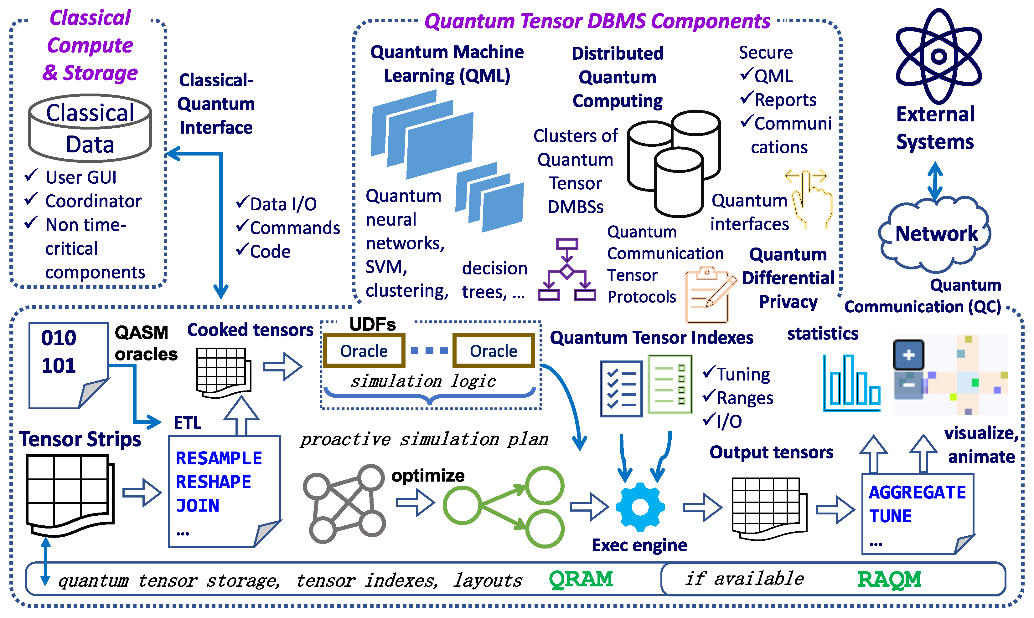
Now, with solid theoretical footing for the future Quantum Array (Tensor) DBMS capabilities, let us holistically describe an architecture of a future Quantum Array (Tensor) DBMS. To date, simulation is the most complex workload for an Array (Tensor) DBMS and the most diverse in the sense of the scope and variety of Array (Tensor) DBMS functions utilized [65,66]. Hence, we illustrate our holistic vision using an end-to-end complex Array (Tensor) DBMS simulation pipeline, Figure 24. This example can also serve as a roadmap or research plan. Obviously, the presented architecture may and should undergo subsequent refinements and maybe even substantial changes reflecting the development of quantum computing, memory, machines, transmission, and other related knowledge domains. However, it is important to start early, right now, by developing first versions of Quantum Array (Tensor) DBMSs based on the theoretical framework that we already have and keeping in pace with quantum research and industry advancements.

Most contemporary related work implicitly or explicitly assumes that a quantum superposition in a quantum register constitutes a database [169]. This is similar to treating the contents of a CPU register as a database without mentioning any I/O. Instead, we devote special attention to in-memory Quantum Array (Tensor) DBMS capabilities. Array (tensor) data can be stored in a classical DBMS component, in QRAM/RAQM which can be the next memory hierarchy level after quantum registers (along with caches; compare classical CPU, RAM, and in-memory database engines), exchanged between classical and quantum Array (Tensor) DBMS components, as well as via quantum communication.

The user starts with a GUI (Graphical User Interface) on a classical machine that serves as a coordinator and executor of non time-critical tasks. The coordinator parses UDFs (User Defined Functions) in the Array (Tensor) DBMS native language [66] and compiles them to quantum circuits. It also generates a proactive simulation plan (PSP) [65,66] by inspecting input array metadata and UDFs. The coordinator fetches an optimized PSP from a quantum component via the classical-quantum interface (CQI). Finally, optimized circuits and arrays are submitted via CQI. We expect probabilistic simulations to have a superpolynomial speedup compared to a classical machine (S2C2M) [208,209,210].

Figure 24. Example of a Quantum Array (Tensor) DBMS running physical simulations together with its prospective classical and quantum components.

Figure 24. Example of a Quantum Array (Tensor) DBMS running physical simulations together with its prospective classical and quantum components.

The procedure is the same for ETL (Extract, Transform, Load), simulation, deriving simulation statistics, and visualization, but ordinary execution plans can be submitted instead of a PSP. Not all array data can fit into the quantum part, so the coordinator splits a PSP into parts that operate on at most a given threshold of array volume that is possible to predict, as we have strict formal definitions of array operations. In addition, it tends to minimize the number and volume of CQI interactions.

The user cooks arrays during the ETL phase by submitting array transformation queries, e.g., resample, reshape, join, that run in S2C2M. The results may go to the classical storage and fetched later if their is no sufficient space in QRAM or RAQM. Recall that Quantum Array (Tensor) DBMSs can also work on data that has been generated inside a quantum machine and is already in a quantum register or quantum memory, not retrieved via CQI. To speedup simulations or certain queries, the user (or the Array (Tensor) DBMS automatically) will create quantum array indexes, Section 4.9.

Finally, the user can investigate input/output data visually or compute statistics via aggregation or more sophisticated operations, e.g., tune [12]. Complex rendering can be performed on the classical side, but the quantum side has the potential to be more beneficial in rapid-response scenarios. Arrays can be exchanged between Quantum Array (Tensor) DBMSs and external systems via quantum communication.

We have outlined the architecture of a future Quantum Array (Tensor) DBMS based on the most complex workload for a contemporary classical Array (Tensor) DBMS. A more comprehensive sketch can include quantum machine learning (QML) [211,212,213,214,215], distributed quantum computing (DQC) [216,217], quantum differential privacy (QDF) [218,219], as well as quantum communication (QC) [220,221,222]. These subareas are very promising within quantum computing. However, some areas are just paving their ways to Array (Tensor) DBMSs, for example, machine learning [8,28,31]. Therefore, Array (Tensor) DBMSs have an opportunity to become even more involved in the rapidly growing field of R&D at early stages, gaining the respective benefits of a timely start: quantum computing can additionally motivate integrating QML and other capabilities into Array (Tensor) DBMSs, making them quantum-ready or quantum-native solutions.

QC promise to provide fast and secure data exchange. Quantum Array (Tensor) DBMSs can leverage QC to move sensitive data between each other and external systems. Array (Tensor) DBMSs utilize open, standardized network protocols like Web Tile Map Service (WMTS) [223] to provide array tiles to multiple concurrent users [9,63]. Currently used protocols can be revised to integrate better with QC and utilize its benefits.

In addition, QC, QML, DQC, and quantum computing in general can be especially helpful in scenarios where immediate, small responses that result from massive computations are desired. For example, consider a typical array (tensor) tile which is shaped $256\times 256$. This means that we need a register of a small number of qubits to process a single tile (or a strip in the Quantum Array (Tensor) DBMS Data Model, Section 4.5). We can provide users a small, assembly-like UDF language to specify operations that they would like to run on the tiles (strips). In addition, such operations may be hard-coded and used in extreme scenarios like disaster monitoring, rapid response, and medical diagnosis. Note that as we would have a language tailored to existing quantum gates, we do not deal with arbitrary functions. Hence, we can compile and submit time-critical computations to quantum computers using our UDFs. This application can be one of the most representative, as it is both immediately practical and does not require a large number of qubits to start experimenting with this application.

UDFs in Array (Tensor) DBMSs are under active research. Most Array (Tensor) DBMSs accept UDFs in Python/C++ which are black boxes that cannot be optimized [22]. However, recently, the first native UDF language for array DBMSs has been introduced in [17]. Window query optimizations for UDFs were presented in [224]. Certainly, diverse quantum compiler optimization techniques are applicable together with multi-tenancy optimization and joint (shared) execution for future quantum UDFs.

DQC can enable building clusters that consist of multiple Quantum Array (Tensor) DBMSs. Note that even new quantum-tailored communication interfaces are being developed, for example, QMPI [217] which is a quantum version of the well-known Message Passing Interface (MPI). Undoubtedly, we include DQC as an enabling technology for Quantum Array (Tensor) DBMSs, because a Quantum Array (Tensor) DBMS would be able to immediately utilize DQC once it becomes mature to reach the same goals as perceived by classical distributed Array (Tensor) DBMSs when launched on a computer cluster [17,67].

Array (Tensor) DBMSs are attractive for machine learning due to their data model that natively operates on arrays (tensors) – one of the key entities in machine learning and data science. In addition, if an Array (Tensor) DBMS has rich built-in machine learning capabilities, it will be possible to avoid costly movements of potentially massive array (tensor) data between systems to perform data engineering coupled with machine learning. In this case, QML inside Quantum Array (Tensor) DBMSs is a natural followup of the aforementioned current efforts with a strong perspective. Quantum Convolutional Neural Networks [225,226,227,228] can deserve special attention from Array (Tensor) DBMS architects and developers, because they can be applicable to Earth array (tensor) data types that currently enjoy the most frequent utilization in Array (Tensor) DBMS workloads, Section 6.1.1, especially if such Earth data happens to be already inside a quantum machine.

7. Concluding Remarks

The journey of Array (Tensor) DBMSs to the area of Quantum Computing has just begun. They meet beautiful theory there, help to energize myriads of Earth science applications, and have a clear path forward. We have introduced a quantum array data model and quantum array approaches to a set of Array (Tensor) DBMS challenges that result in exponential reduction in the runtime computational complexity at the information theoretical level: quantum $O\left(n\right)$ vs. classical $O\left(2^n\right)$. This proves that Array (Tensor) DBMSs and Earth data engineering are a good target for quantum computing which can enable unprecedented speedups intrinsically. It is especially attractive to utilize Array (Tensor) DBMSs for data that is already inside a quantum computer, e.g., as a result of previous activity like simulations. We showcased quantum memory and quantum computing potentials for Array (Tensor) DBMSs, as well as contributed by reasoning about quantum array-tailored memory operations, as current literature lacks these aspects.

Quantum Gantt charts (QGantt charts) and Quantum Network Diagrams (QND) deserve a special note as they represent a new and comprehensive way to illustrate quantum computing and quantum memory operations in a static format. We used QGantt charts to demonstrate standard quantum techniques, unrelated to Quantum Array (Tensor) DBMSs, as well as to explain our new approaches. We accompanied our algorithms with QGantt charts to show that they are widely applicable for research, development, and educational purposes, especially those that benefit from seeing exact numerical values of superposition terms and easily tracking of inputs/outputs of quantum operations in detail.

Nevertheless, much still needs to be done: we holistically outlined key challenges and opportunities in building a complete Quantum Array (Tensor) DBMS, formed an intuition on how Quantum Array (Tensor) DBMSs may be designed, and provided a roadmap for future Quantum Array (Tensor) DBMS R&D. Of course, we expect that the proposed solutions and our vision will be further improved, as these represent the first steps in Quantum Array (Tensor) DBMSs. The goal and the rewards shine so brightly and appealingly, that they serve as a strong source of motivation for future work.

References

1. Donoho, D. 50 years of data science. J. Comput. Graph. Stat. 2017, 26, 745–766. [Google Scholar]
2. Chai, C.P. The importance of data cleaning: Three visualization examples. Chance 2020, 33, 4–9. [Google Scholar]
3. ECMWF. 2022. Available online: https://www.ecmwf.int/en/computing/our-facilities/data-handling-system (accessed on 22 August 2024).
4. Sentinel Data Access Annual Report. 2021. Available online: https://sentinels.copernicus.eu/web/sentinel/-/copernicus-sentinel-data-access-annual-report-2021 (accessed on 22 August 2024).
5. Nativi, S.; Caron, J.; Domenico, B.; Bigagli, L. Unidata’s Common Data Model mapping to the ISO 19123 Data Model. Earth Sci. Inform. 2008, 1, 59–78. [Google Scholar]
6. Balaji, V.; Adcroft, A.; Liang, Z. Gridspec: A standard for the description of grids used in Earth System models. arXiv 2019, arXiv:1911.08638. [Google Scholar]
7. Rusu, F. Multidimensional array data management. Found. Trends® Databases 2023, 12, 69–220. [Google Scholar]
8. Rodriges Zalipynis, R.A. Array DBMS: Past, Present, and (Near) Future. Proc. VLDB Endow. 2021, 14, 3186–3189. [Google Scholar]
9. Baumann, P.; Misev, D.; Merticariu, V.; Huu, B.P. Array databases: Concepts, standards, implementations. J. Big Data 2021, 8, 1–61. [Google Scholar]
10. Kingsmore, S.F.; Smith, L.D.; Kunard, C.M.; Bainbridge, M.; Batalov, S.; Benson, W.; Blincow, E.; Caylor, S.; Chambers, C.; Del Angel, G.; et al. A genome sequencing system for universal newborn screening, diagnosis, and precision medicine for severe genetic diseases. Am. J. Hum. Genet. 2022, 109, 1605–1619. [Google Scholar]
11. Askenazi, M.; Ben Hamidane, H.; Graumann, J. The arc of Mass Spectrometry Exchange Formats is long, but it bends toward HDF5. Mass Spectrom. Rev. 2017, 36, 668–673. [Google Scholar]
12. Rodriges Zalipynis, R.A. BitFun: Fast Answers to Queries with Tunable Functions in Geospatial Array DBMS. Proc. VLDB Endow. 2020, 13, 2909–2912. [Google Scholar]
13. Horlova, O.; Kaitoua, A.; Ceri, S. Array-based Data Management for Genomics. In Proceedings of the 2020 IEEE 36th International Conference on Data Engineering (ICDE), Dallas, TX, USA, 20–24 April 2020; pp. 109–120. [Google Scholar]
14. Masseroli, M.; Canakoglu, A.; Pinoli, P.; Kaitoua, A.; Gulino, A.; Horlova, O.; Nanni, L.; Bernasconi, A.; Perna, S.; Stamoulakatou, E.; et al. Processing of big heterogeneous genomic datasets for tertiary analysis of Next Generation Sequencing data. Bioinformatics 2019, 35, 729–736. [Google Scholar]
15. Rodriges Zalipynis, R.A. Generic Distributed In Situ Aggregation for Earth Remote Sensing Imagery. In Proceedings of the International Conference on Analysis of Images, Social Networks and Texts, Moscow, Russia, 5–7 July 2018; LNCS. Springer: Cham, Switzerland, 2018; Volume 11179, pp. 331–342. [Google Scholar]
16. Xing, H.; Agrawal, G. COMPASS: Compact array storage with value index. In Proceedings of the 30th International Conference on Scientific and Statistical Database Management, Bozen-Bolzano, Italy, 9–11 July 2018; pp. 1–12. [Google Scholar]
17. Rodriges Zalipynis, R.A. ChronosDB: Distributed, File Based, Geospatial Array DBMS. Proc. VLDB Endow. 2018, 11, 1247–1261. [Google Scholar]
18. Deaton, A.M.; Parker, M.M.; Ward, L.D.; Flynn-Carroll, A.O.; BonDurant, L.; Hinkle, G.; Akbari, P.; Lotta, L.A. Gene-level analysis of rare variants in 379,066 whole exome sequences identifies an association of GIGYF1 loss of function with type 2 diabetes. Sci. Rep. 2021, 11, 21565. [Google Scholar]
19. Ward, L.D.; Tu, H.C.; Quenneville, C.B.; Tsour, S.; Flynn-Carroll, A.O.; Parker, M.M.; Deaton, A.M.; Haslett, P.A.; Lotta, L.A.; Verweij, N.; et al. GWAS of serum ALT and AST reveals an association of SLC30A10 Thr95Ile with hypermanganesemia symptoms. Nat. Commun. 2021, 12, 4571. [Google Scholar]
20. Aleksandrov, M.; Zlatanova, S.; Heslop, D.J. Voxelisation algorithms and data structures: A review. Sensors 2021, 21, 8241. [Google Scholar] [CrossRef]
21. Kim, M.; Lee, H.; Chung, Y.D. Multi-Dimensional Data Compression and Query Processing in Array Databases. IEEE Access 2022, 10, 111528–111544. [Google Scholar]
22. Mehta, P.; Dorkenwald, S.; Zhao, D.; Kaftan, T.; Cheung, A.; Balazinska, M.; Rokem, A.; Connolly, A.; Vanderplas, J.; AlSayyad, Y. Comparative evaluation of big-data systems on scientific image analytics workloads. Proc. VLDB Endow. 2017, 10, 1226–1237. [Google Scholar]
23. Cudre-Mauroux, P.; Kimura, H.; Lim, K.T.; Rogers, J.; Madden, S.; Stonebraker, M.; Zdonik, S.B.; Brown, P.G. SS-DB: A Standard Science DBMS Benchmark. In Proceedings of the XLDB, 2010. Available online: https://people.csail.mit.edu/jennie/_content/research/ssdb_benchmark.pdf (accessed on 22 August 2024).
24. Soroush, E.; Balazinska, M.; Wang, D. ArrayStore: A storage manager for complex parallel array processing. In Proceedings of the 2011 ACM SIGMOD International Conference on Management of Data, Athens, Greece, 12–16 June 2011; pp. 253–264. [Google Scholar]
25. Kim, B.; Koo, K.; Enkhbat, U.; Kim, S.; Kim, J.; Moon, B. M2Bench: A Database Benchmark for Multi-Model Analytic Workloads. Proc. VLDB Endow. 2022, 16, 747–759. [Google Scholar]
26. Choi, D.; Yoon, H.; Chung, Y.D. ReSKY: Efficient Subarray Skyline Computation in Array Databases. Distrib. Parallel Databases 2022, 40, 261–298. [Google Scholar]
27. Choi, D.; Yoon, H.; Chung, Y.D. Subarray skyline query processing in array databases. In Proceedings of the 33rd International Conference on Scientific and Statistical Database Management, Tampa, FL, USA, 6–7 July 2021; pp. 37–48. [Google Scholar]
28. Villarroya, S.; Baumann, P. On the Integration of Machine Learning and Array Databases. In Proceedings of the 2020 IEEE 36th International Conference on Data Engineering (ICDE), Dallas, TX, USA, 20–24 April 2020; pp. 1786–1789. [Google Scholar]
29. Rodriges Zalipynis, R.A. Towards Machine Learning in Distributed Array DBMS: Networking Considerations. In Proceedings of the Machine Learning for Networking: Third International Conference, MLN 2020, Paris, France, 24–26 November 2020; LNCS. Springer: Cham, Switzerland, 2021; Volume 12629, pp. 284–304. [Google Scholar]
30. Ordonez, C.; Zhang, Y.; Johnsson, S.L. Scalable machine learning computing a data summarization matrix with a parallel array DBMS. Distrib. Parallel Databases 2019, 37, 329–350. [Google Scholar]
31. Villarroya, S.; Baumann, P. A survey on machine learning in array databases. Appl. Intell. 2023, 53, 9799–9822. [Google Scholar]
32. Alam, M.M.; Torgo, L.; Bifet, A. A survey on spatio-temporal data analytics systems. ACM Comput. Surv. 2022, 54, 1–38. [Google Scholar]
33. Xu, C.; Du, X.; Fan, X.; Giuliani, G.; Hu, Z.; Wang, W.; Liu, J.; Wang, T.; Yan, Z.; Zhu, J.; et al. Cloud-based storage and computing for remote sensing big data: A technical review. Int. J. Digit. Earth 2022, 15, 1417–1445. [Google Scholar]
34. Lewis, A.; Oliver, S.; Lymburner, L.; Evans, B.; Wyborn, L.; Mueller, N.; Raevksi, G.; Hooke, J.; Woodcock, R.; Sixsmith, J.; et al. The Australian Geoscience Data Cube—Foundations and lessons learned. Remote Sens. Environ. 2017, 202, 276–292. [Google Scholar]
35. Baumann, P.; Misev, D.; Merticariu, V.; Huu, B.P.; Bell, B. DataCubes: A technology survey. In Proceedings of the IGARSS 2018-2018 IEEE International Geoscience and Remote Sensing Symposium, Valencia, Spain, 22–27 July 2018; pp. 430–433. [Google Scholar]
36. Baumann, P. Towards a Model-Driven Datacube Analytics Language. In Proceedings of the 2021 IEEE International Conference on Big Data (Big Data), Orlando, FL, USA, 15–18 December 2021; pp. 3740–3746. [Google Scholar]
37. Mahecha, M.D.; Gans, F.; Brandt, G.; Christiansen, R.; Cornell, S.E.; Fomferra, N.; Kraemer, G.; Peters, J.; Bodesheim, P.; Camps-Valls, G.; et al. Earth system data cubes unravel global multivariate dynamics. Earth Syst. Dyn. 2020, 11, 201–234. [Google Scholar]
38. Baumann, P.; Misev, D. ORBiDANSe: Orbital Big Datacube Analytics Service. In Proceedings of the EGU General Assembly Conference Abstracts, Vienna, Austria, 23–27 May 2022; p. EGU22-13002. [Google Scholar]
39. Rivera, G.; Porras, R.; Florencia, R.; Sánchez-Solís, J.P. LiDAR applications in precision agriculture for cultivating crops: A review of recent advances. Comput. Electron. Agric. 2023, 207, 107737. [Google Scholar]
40. Su, J.; Zhu, X.; Li, S.; Chen, W.H. AI meets UAVs: A survey on AI empowered UAV perception systems for precision agriculture. Neurocomputing 2023, 518, 242–270. [Google Scholar]
41. Pande, C.B.; Moharir, K.N. Application of hyperspectral remote sensing role in precision farming and sustainable agriculture under climate change: A review. In Climate Change Impacts on Natural Resources, Ecosystems and Agricultural Systems; Springer: Berlin/Heidelberg, Germany, 2023; pp. 503–520. [Google Scholar]
42. Luo, Y.; Huang, H.; Roques, A. Early monitoring of forest wood-boring pests with remote sensing. Annu. Rev. Entomol. 2023, 68, 277–298. [Google Scholar]
43. Massey, R.; Berner, L.T.; Foster, A.C.; Goetz, S.J.; Vepakomma, U. Remote Sensing Tools for Monitoring Forests and Tracking Their Dynamics. In Boreal Forests in the Face of Climate Change: Sustainable Management; Springer: Berlin/Heidelberg, Germany, 2023; pp. 637–655. [Google Scholar]
44. Yu, D.; Fang, C. Urban Remote Sensing with Spatial Big Data: A Review and Renewed Perspective of Urban Studies in Recent Decades. Remote Sens. 2023, 15, 1307. [Google Scholar] [CrossRef]
45. Li, F.; Yigitcanlar, T.; Nepal, M.; Nguyen, K.; Dur, F. Machine Learning and Remote Sensing Integration for Leveraging Urban Sustainability: A Review and Framework. Sustain. Cities Soc. 2023, 96, 104653. [Google Scholar]
46. Adjovu, G.E.; Stephen, H.; James, D.; Ahmad, S. Overview of the Application of Remote Sensing in Effective Monitoring of Water Quality Parameters. Remote Sens. 2023, 15, 1938. [Google Scholar] [CrossRef]
47. Liu, Z.; Xu, J.; Liu, M.; Yin, Z.; Liu, X.; Yin, L.; Zheng, W. Remote sensing and geostatistics in urban water-resource monitoring: A review. Mar. Freshw. Res. 2023, 74, 747–765. [Google Scholar]
48. Kurniawan, R.; Alamsyah, A.R.B.; Fudholi, A.; Purwanto, A.; Sumargo, B.; Gio, P.U.; Wongsonadi, S.K.; Susanto, A.E.H. Impacts of industrial production and air quality by remote sensing on nitrogen dioxide concentration and related effects: An econometric approach. Environ. Pollut. 2023, 334, 122212. [Google Scholar]
49. Abu El-Magd, S.; Soliman, G.; Morsy, M.; Kharbish, S. Environmental hazard assessment and monitoring for air pollution using machine learning and remote sensing. Int. J. Environ. Sci. Technol. 2023, 20, 6103–6116. [Google Scholar]
50. Sudmanns, M.; Augustin, H.; Killough, B.; Giuliani, G.; Tiede, D.; Leith, A.; Yuan, F.; Lewis, A. Think global, cube local: An Earth Observation Data Cube’s contribution to the Digital Earth vision. Big Earth Data 2023, 7, 831–859. [Google Scholar]
51. Mahmood, R.; Zhang, L.; Li, G. Assessing effectiveness of nature-based solution with big earth data: 60 years mangrove plantation program in Bangladesh coast. Ecol. Process. 2023, 12, 11. [Google Scholar]
52. Wang, S.; Wang, J.; Zhan, Q.; Zhang, L.; Yao, X.; Li, G. A unified representation method for interdisciplinary spatial earth data. Big Earth Data 2023, 7, 126–145. [Google Scholar]
53. Rodriges Zalipynis, R.A.; Pozdeev, E.; Bryukhov, A. Array DBMS and Satellite Imagery: Towards Big Raster Data in the Cloud. In Proceedings of the International Conference on Analysis of Images, Social Networks and Texts, Moscow, Russia, 27–29 July 2017; LNCS. Volume 10716, pp. 267–279. [Google Scholar]
54. Ladra, S.; Paramá, J.R.; Silva-Coira, F. Scalable and queryable compressed storage structure for raster data. Inf. Syst. 2017, 72, 179–204. [Google Scholar]
55. Leclercq, É.; Gillet, A.; Grison, T.; Savonnet, M. Polystore and Tensor Data Model for Logical Data Independence and Impedance Mismatch in Big Data Analytics. In LNCS; Springer: Berlin/Heidelberg, Germany, 2019; pp. 51–90. [Google Scholar]
56. Papadopoulos, S.; Datta, K.; Madden, S.; Mattson, T. The TileDB Array Data Storage Manager. Proc. VLDB Endow. 2016, 10, 349–360. [Google Scholar]
57. Rodriges Zalipynis, R.A. ChronosDB in Action: Manage, Process, and Visualize Big Geospatial Arrays in the Cloud. In Proceedings of the 2019 International Conference on Management of Data, Amsterdam, The Netherlands, 30 June–5 July 2019; pp. 1985–1988. [Google Scholar]
58. Zhao, W.; Rusu, F.; Dong, B.; Wu, K.; Nugent, P. Incremental view maintenance over array data. In Proceedings of the 2017 ACM International Conference on Management of Data, Chicago, IL, USA, 14–19 May 2017; pp. 139–154. [Google Scholar]
59. Zhao, W.; Rusu, F.; Dong, B.; Wu, K. Similarity join over array data. In Proceedings of the 2016 International Conference on Management of Data, San Francisco, CA, USA, 26 June–1 July 2016; pp. 2007–2022. [Google Scholar]
60. Zhao, W.; Rusu, F.; Dong, B.; Wu, K.; Ho, A.Y.; Nugent, P. Distributed caching for processing raw arrays. In Proceedings of the 30th International Conference on Scientific and Statistical Database Management, Bozen-Bolzano, Italy, 9–11 July 2018. [Google Scholar]
61. Rodriges Zalipynis, R.A. FastMosaic in Action: A New Mosaic Operator for Array DBMSs. Proc. VLDB Endow. 2023, 16, 3938–3941. [Google Scholar]
62. Kilsedar, C.E.; Brovelli, M.A. Multidimensional visualization and processing of big open urban geospatial data on the web. ISPRS Int. J.-Geo-Inf. 2020, 9, 434. [Google Scholar]
63. Rodriges Zalipynis, R.A.; Terlych, N. WebArrayDB: A Geospatial Array DBMS in Your Web Browser. Proc. VLDB Endow. 2022, 15, 3622–3625. [Google Scholar]
64. Battle, L.; Chang, R.; Stonebraker, M. Dynamic prefetching of data tiles for interactive visualization. In Proceedings of the 2016 International Conference on Management of Data, San Francisco, CA, USA, 26 June–1 July 2016; pp. 1363–1375. [Google Scholar]
65. Rodriges Zalipynis, R.A. SimDB in Action: Road Trafic Simulations Completely Inside Array DBMS. Proc. VLDB Endow. 2022, 15, 3742–3745. [Google Scholar]
66. Rodriges Zalipynis, R.A. Convergence of Array DBMS and Cellular Automata: A Road Traffic Simulation Case. In Proceedings of the 2021 International Conference on Management of Data, Xi’an, China, 20–25 June 2021; pp. 2399–2403. [Google Scholar]
67. Cudre-Mauroux, P.; Kimura, H.; Lim, K.T.; Rogers, J.; Simakov, R.; Soroush, E.; Velikhov, P.; Wang, D.L.; Balazinska, M.; Becla, J.; et al. A demonstration of SciDB: A science-oriented DBMS. Proc. VLDB Endow. 2009, 2, 1534–1537. [Google Scholar]
68. Gorelick, N.; Hancher, M.; Dixon, M.; Ilyushchenko, S.; Thau, D.; Moore, R. Google Earth Engine: Planetary-scale geospatial analysis for everyone. Remote Sens. Environ. 2017, 202, 18–27. [Google Scholar]
69. Zhao, Q.; Yu, L.; Li, X.; Peng, D.; Zhang, Y.; Gong, P. Progress and trends in the application of Google Earth and Google Earth Engine. Remote Sens. 2021, 13, 3778. [Google Scholar] [CrossRef]
70. Wang, Y.; Nandi, A.; Agrawal, G. SAGA: Array Storage as a DB with Support for Structural Aggregations. In Proceedings of the 26th International Conference on Scientific and Statistical Database Management, Aalborg, Denmark, 30 June–2 July 2014. [Google Scholar]
71. Baumann, P.; Mazzetti, P.; Ungar, J.; Barbera, R.; Barboni, D.; Beccati, A.; Bigagli, L.; Boldrini, E.; Bruno, R.; Calanducci, A.; et al. Big data analytics for Earth sciences: The EarthServer approach. Int. J. Digit. Earth 2016, 9, 3–29. [Google Scholar]
72. GeoTrellis. 2024. Available online: https://geotrellis.io/ (accessed on 22 August 2024).
73. Dask. 2024. Available online: https://dask.org/ (accessed on 22 August 2024).
74. Microsoft Planetary Computer. 2024. Available online: https://planetarycomputer.microsoft.com/ (accessed on 22 August 2024).
75. Earth Engine|Google Cloud. 2024. Available online: https://cloud.google.com/earth-engine (accessed on 22 August 2024).
76. Rodriges Zalipynis, R.A. Evaluating Array DBMS Compression Techniques for Big Environmental Datasets. In Proceedings of the 2019 10th IEEE International Conference on Intelligent Data Acquisition and Advanced Computing Systems: Technology and Applications (IDAACS), Metz, France, 18–21 September 2019; Volume 2, pp. 859–863. [Google Scholar]
77. Mainzer, J.; Fortner, N.; Heber, G.; Pourmal, E.; Koziol, Q.; Byna, S.; Paterno, M. Sparse Data Management in HDF5. In Proceedings of the 2019 IEEE/ACM 1st Annual Workshop on Large-Scale Experiment-in-the-Loop Computing (XLOOP), Denver, CO, USA, 18 November 2019; pp. 20–25. [Google Scholar]
78. Cheng, Y.; Zhao, W.; Rusu, F. Bi-Level Online Aggregation on Raw Data. In Proceedings of the 29th International Conference on Scientific and Statistical Database Management, Chicago, IL, USA, 27–29 June 2017. [Google Scholar]
79. Blanas, S.; Wu, K.; Byna, S.; Dong, B.; Shoshani, A. Parallel data analysis directly on scientific file formats. In Proceedings of the 2014 ACM SIGMOD International Conference on Management of Data, New York, NY, USA, 22–27 June 2014. [Google Scholar]
80. Su, Y.; Agrawal, G. Supporting user-defined subsetting and aggregation over parallel NetCDF datasets. In Proceedings of the 2012 12th IEEE/ACM International Symposium on Cluster, Cloud and Grid Computing CCGrid, Ottawa, ON, Canada, 13–16 May 2012; pp. 212–219. [Google Scholar]
81. Rodriges Zalipynis, R.A. Distributed In Situ Processing of Big Raster Data in the Cloud. In Proceedings of the Perspectives of System Informatics, Moscow, Russia, 27–29 June 2017; LNCS. Springer: Cham, Switzerland, 2018; Volume 10742, pp. 337–351. [Google Scholar]
82. Xing, H.; Agrawal, G. Accelerating array joining with integrated value-index. In Proceedings of the 31st International Conference on Scientific and Statistical Database Management, Vienna, Austria, 7–9 July 2020; pp. 145–156. [Google Scholar]
83. Choi, D.; Park, C.S.; Chung, Y.D. Progressive top-k subarray query processing in array databases. Proc. VLDB Endow. 2019, 12, 989–1001. [Google Scholar]
84. Azure Quantum Homepage. 2024. Available online: https://quantum.microsoft.com/ (accessed on 22 August 2024).
85. Cloud Quantum Computing Service—Amazon Braket—AWS. 2024. Available online: https://aws.amazon.com/braket (accessed on 22 August 2024).
86. IBM Quantum Computing. 2024. Available online: https://www.ibm.com/quantum (accessed on 22 August 2024).
87. Google Quantum AI. 2024. Available online: https://quantumai.google/ (accessed on 22 August 2024).
88. Qubit Scorecard. 2024. Available online: https://www.qusecure.com/qubit-scorecard/ (accessed on 22 August 2024).
89. Fujitsu Quantum. 2024. Available online: https://www.fujitsu.com/global/about/research/technology/quantum/ (accessed on 22 August 2024).
90. Atom Computing. 2024. Available online: https://atom-computing.com/ (accessed on 22 August 2024).
91. D-Wave Systems. 2024. Available online: https://www.dwavesys.com/ (accessed on 22 August 2024).
92. D-Wave. D-Wave Announces Availability of 1200+ Qubit Advantage2™ Prototype. 2024. Available online: https://www.dwavesys.com/company/newsroom/press-release/d-wave-announces-availability-of-1-200-qubit-advantage2-prototype/ (accessed on 22 August 2024).
93. IBM 100,000 Qubit Supercomputer. 2023. Available online: www.ibm.com/quantum/blog/100k-qubit-supercomputer (accessed on 22 August 2024).
94. Feynman, R.P. Simulating Physics with Computers. Int. J. Theor. Phys. 1982, 21, 133–153. [Google Scholar]
95. Benioff, P. Quantum mechanical Hamiltonian models of Turing machines. J. Stat. Phys. 1982, 29, 515–546. [Google Scholar]
96. Deutsch, D. Quantum theory, the Church–Turing principle and the universal quantum computer. Proc. R. Soc. Lond. A Math. Phys. Sci. 1985, 400, 97–117. [Google Scholar]
97. Shor, P.W. Algorithms for quantum computation: Discrete logarithms and factoring. In Proceedings of the 35th Annual Symposium on Foundations of Computer Science, Santa Fe, NM, USA, 20–22 November 1994; pp. 124–134. [Google Scholar]
98. Grover, L.K. A fast quantum mechanical algorithm for database search. In Proceedings of the Twenty-Eighth Annual ACM Symposium on Theory of Computing, Philadelphia, PA, USA, 22–24 May 1996; pp. 212–219. [Google Scholar]
99. Chen, J.; Stoudenmire, E.; White, S.R. Quantum Fourier Transform Has Small Entanglement. PRX Quantum 2023, 4, 040318. [Google Scholar]
100. Camps, D.; Van Beeumen, R.; Yang, C. Quantum Fourier transform revisited. Numer. Linear Algebra Appl. 2021, 28, e2331. [Google Scholar]
101. Acampora, G.; Chiatto, A.; Vitiello, A. Genetic algorithms as classical optimizer for the Quantum Approximate Optimization Algorithm. Appl. Soft Comput. 2023, 142, 110296. [Google Scholar]
102. Drias, H.; Drias, Y.; Houacine, N.A.; Bendimerad, L.S.; Zouache, D.; Khennak, I. Quantum OPTICS and deep self-learning on swarm intelligence algorithms for Covid-19 emergency transportation. Soft Comput. 2023, 27, 13181–13200. [Google Scholar]
103. Mukhamedov, F.; Souissi, A.; Hamdi, T.; Andolsi, A. Open quantum random walks and quantum Markov Chains on trees II: The recurrence. Quantum Inf. Process. 2023, 22, 232. [Google Scholar]
104. Ardelean, S.M.; Udrescu, M. Graph coloring using the reduced quantum genetic algorithm. PeerJ Comput. Sci. 2022, 8, e836. [Google Scholar]
105. Gupta, R.; Saxena, D.; Gupta, I.; Makkar, A.; Singh, A.K. Quantum machine learning driven malicious user prediction for cloud network communications. IEEE Netw. Lett. 2022, 4, 174–178. [Google Scholar]
106. Melnikov, A.; Kordzanganeh, M.; Alodjants, A.; Lee, R.K. Quantum machine learning: From physics to software engineering. Adv. Phys. X 2023, 8, 2165452. [Google Scholar]
107. Biasse, J.F.; Bonnetain, X.; Kirshanova, E.; Schrottenloher, A.; Song, F. Quantum algorithms for attacking hardness assumptions in classical and post-quantum cryptography. IET Inf. Secur. 2023, 17, 171–209. [Google Scholar]
108. Herman, D.; Googin, C.; Liu, X.; Sun, Y.; Galda, A.; Safro, I.; Pistoia, M.; Alexeev, Y. Quantum computing for finance. Nat. Rev. Phys. 2023, 5, 450–465. [Google Scholar]
109. Cordier, B.A.; Sawaya, N.P.; Guerreschi, G.G.; McWeeney, S.K. Biology and medicine in the landscape of quantum advantages. J. R. Soc. Interface 2022, 19, 20220541. [Google Scholar]
110. Huang, D.; Wang, M.; Wang, J.; Yan, J. A survey of quantum computing hybrid applications with brain-computer interface. Cogn. Robot. 2022, 2, 64–176. [Google Scholar]
111. Ullah, M.H.; Eskandarpour, R.; Zheng, H.; Khodaei, A. Quantum computing for smart grid applications. IET Gener. Transm. Distrib. 2022, 16, 4239–4257. [Google Scholar]
112. Lloyd, S.; Mohseni, M.; Rebentrost, P. Quantum principal component analysis. Nat. Phys. 2014, 10, 631–633. [Google Scholar]
113. Fritsch, K.; Scherzinger, S. Solving Hard Variants of Database Schema Matching on Quantum Computers. Proc. VLDB Endow. 2023, 16, 3990–3993. [Google Scholar]
114. Groppe, S.; Groppe, J.; Çalıkyılmaz, U.; Winker, T.; Gruenwal, L. Quantum data management and quantum machine learning for data management: State-of-the-art and open challenges. In Proceedings of the International Conference on Intelligent Systems and Machine Learning, Guangzhou, China, 5–7 August 2022; Springer: Berlin/Heidelberg, Germany, 2022; pp. 252–261. [Google Scholar]
115. Figgatt, C.; Maslov, D.; Landsman, K.A.; Linke, N.M.; Debnath, S.; Monroe, C. Complete 3-qubit Grover search on a programmable quantum computer. Nat. Commun. 2017, 8, 1918. [Google Scholar]
116. Zajac, M.; Störl, U. Towards quantum-based Search for industrial Data-driven Services. In Proceedings of the 2022 IEEE International Conference on Quantum Software (QSW), Barcelona, Spain, 10–16 July 2022; pp. 38–40. [Google Scholar]
117. Trummer, I.; Koch, C. Multiple Query Optimization on the D-Wave 2X Adiabatic Quantum Computer. arXiv 2015, arXiv:1510.06437. [Google Scholar]
118. Schönberger, M. Applicability of quantum computing on database query optimization. In Proceedings of the 2022 International Conference on Management of Data, Philadelphia, PA, USA, 12–17 June 2022; pp. 2512–2514. [Google Scholar]
119. Fankhauser, T.; Solèr, M.E.; Füchslin, R.M.; Stockinger, K. Multiple Query Optimization using a Gate-Based Quantum Computer. IEEE Access 2023, 11, 114043. [Google Scholar]
120. Çalikyilmaz, U.; Groppe, S.; Groppe, J.; Winker, T.; Prestel, S.; Shagieva, F.; Arya, D.; Preis, F.; Gruenwald, L. Opportunities for quantum acceleration of databases: Optimization of queries and transaction schedules. Proc. VLDB Endow. 2023, 16, 2344–2353. [Google Scholar]
121. Albert Einstein Quote. 2024. Available online: https://www.azquotes.com/quote/905255 (accessed on 22 August 2024).
122. Wootters, W.K.; Zurek, W.H. A single quantum cannot be cloned. Nature 1982, 299, 802–803. [Google Scholar]
123. Aaronson, S.; Gottesman, D. Improved simulation of stabilizer circuits. Phys. Rev. A 2004, 70, 052328. [Google Scholar]
124. Kitaev, A.Y.; Shen, A.; Vyalyi, M.N. Classical and Quantum Computation; Number 47; American Mathematical Soc.: Washington, DC, USA, 2002. [Google Scholar]
125. Shor, P.W. Polynomial-time algorithms for prime factorization and discrete logarithms on a quantum computer. SIAM Rev. 1999, 41, 303–332. [Google Scholar]
126. IonQ Glossary. 2024. Available online: https://ionq.com/resources/glossary (accessed on 22 August 2024).
127. IonQ|Trapped Ion Quantum Computing. 2024. Available online: https://ionq.com/ (accessed on 22 August 2024).
128. QuEra. 2024. Available online: https://www.quera.com/ (accessed on 22 August 2024).
129. Rigetti Computing. 2024. Available online: https://www.rigetti.com/ (accessed on 22 August 2024).
130. Oxford Quantum Circuits. 2024. Available online: https://oxfordquantumcircuits.com/ (accessed on 22 August 2024).
131. Cormen, T.H.; Leiserson, C.E.; Rivest, R.L.; Stein, C. Introduction to Algorithms; MIT Press: Cambridge, MA, USA, 2022. [Google Scholar]
132. Kaye, P.; Laflamme, R.; Mosca, M. An Introduction to Quantum Computing; OUP Oxford: Oxford, UK, 2006. [Google Scholar]
133. Kaiser, S.C.; Granade, C. Learn Quantum Computing with Python and Q#: A Hands-on Approach; Simon and Schuster: New York, NY, USA, 2021. [Google Scholar]
134. Vos, J. Quantum Computing in Action; Simon and Schuster: New York, NY, USA, 2022. [Google Scholar]
135. Silva, V. Practical Quantum Computing for Developers: Programming Quantum Rigs in the Cloud Using Python, Quantum Assembly Language and IBM QExperience; Apress: New York, NY, USA, 2018. [Google Scholar]
136. Combarro, E.F.; Gonzalez-Castillo, S.; Di Meglio, A. A Practical Guide to Quantum Machine Learning and Quantum Optimization: Hands-on Approach to Modern Quantum Algorithms; Packt: Birmingham, UK, 2023. [Google Scholar]
137. Q# Programming Language. 2024. Available online: https://github.com/microsoft/qsharp-language (accessed on 22 August 2024).
138. OpenQASM. 2024. Available online: https://openqasm.com/ (accessed on 22 August 2024).
139. Quantum Computing API for Java. 2024. Available online: https://github.com/redfx-quantum/strange (accessed on 22 August 2024).
140. QuTiP—Quantum Toolbox in Python. 2024. Available online: https://qutip.org/ (accessed on 22 August 2024).
141. Giovannetti, V.; Lloyd, S.; Maccone, L. Quantum random access memory. Phys. Rev. Lett. 2008, 100, 160501. [Google Scholar]
142. Zidan, M.; Abdel-Aty, A.H.; Khalil, A.; Abdel-Aty, M.; Eleuch, H. A novel efficient quantum random access memory. IEEE Access 2021, 9, 151775–151780. [Google Scholar]
143. Park, D.K.; Petruccione, F.; Rhee, J.K.K. Circuit-based quantum random access memory for classical data. Sci. Rep. 2019, 9, 3949. [Google Scholar]
144. Phalak, K.; Chatterjee, A.; Ghosh, S. Quantum random access memory for dummies. Sensors 2023, 23, 7462. [Google Scholar] [CrossRef]
145. Liu, C.; Wang, M.; Stein, S.A.; Ding, Y.; Li, A. Quantum Memory: A Missing Piece in Quantum Computing Units. arXiv 2023, arXiv:2309.14432. [Google Scholar]
146. Jaques, S.; Rattew, A.G. QRAM: A survey and critique. arXiv 2023, arXiv:2305.10310. [Google Scholar]
147. Xu, S.; Hann, C.T.; Foxman, B.; Girvin, S.M.; Ding, Y. Systems architecture for quantum random access memory. In Proceedings of the 56th Annual IEEE/ACM International Symposium on Microarchitecture, Toronto, ON, Canada, 28 October–1 November 2023; pp. 526–538. [Google Scholar]
148. Hoefler, T.; Häner, T.; Troyer, M. Disentangling hype from practicality: On realistically achieving quantum advantage. Commun. ACM 2023, 66, 82–87. [Google Scholar]
149. Customer Success Stories D-Wave. 2024. Available online: https://www.dwavesys.com/learn/customer-success-stories/ (accessed on 22 August 2024).
150. Wang, C.; Li, X.; Xu, H.; Li, Z.; Wang, J.; Yang, Z.; Mi, Z.; Liang, X.; Su, T.; Yang, C.; et al. Towards practical quantum computers: Transmon qubit with a lifetime approaching 0.5 milliseconds. npj Quantum Inf. 2022, 8, 3. [Google Scholar]
151. Pal, S.; Bhattacharya, M.; Lee, S.S.; Chakraborty, C. Quantum computing in the next-generation computational biology landscape: From protein folding to molecular dynamics. Mol. Biotechnol. 2024, 66, 163–178. [Google Scholar]
152. Bharti, K.; Cervera-Lierta, A.; Kyaw, T.H.; Haug, T.; Alperin-Lea, S.; Anand, A.; Degroote, M.; Heimonen, H.; Kottmann, J.S.; Menke, T.; et al. Noisy intermediate-scale quantum algorithms. Rev. Mod. Phys. 2022, 94, 015004. [Google Scholar]
153. Kazmina, A.S.; Zalivako, I.V.; Borisenko, A.S.; Nemkov, N.A.; Nikolaeva, A.S.; Simakov, I.A.; Kuznetsova, A.V.; Egorova, E.Y.; Galstyan, K.P.; Semenin, N.V.; et al. Demonstration of a parity-time-symmetry-breaking phase transition using superconducting and trapped-ion qutrits. Phys. Rev. A 2024, 109, 032619. [Google Scholar]
154. IBM Quantum Composer. 2024. Available online: https://quantum.ibm.com/composer/files/new (accessed on 22 August 2024).
155. Barthe, A.; Grossi, M.; Tura, J.; Dunjko, V. Bloch Sphere Binary Trees: A method for the visualization of sets of multi-qubit systems pure states. arXiv 2023, arXiv:2302.02957. [Google Scholar]
156. Koczor, B.; Zeier, R.; Glaser, S.J. Fast computation of spherical phase-space functions of quantum many-body states. Phys. Rev. A 2020, 102, 062421. [Google Scholar]
157. IBM Quantum Computer with over 1000 Qubits. 2023. Available online: https://www.nature.com/articles/d41586-023-03854-1 (accessed on 22 August 2024).
158. IBM Q-Sphere. 2024. Available online: https://quantum-computing.ibm.com/composer/docs/iqx/visualizations#q-sphere-view (accessed on 22 August 2024).
159. Migdał, P. Symmetries and self-similarity of many-body wavefunctions. arXiv 2014, arXiv:1412.6796. [Google Scholar]
160. IBM Qiskit Circuit Visualization. 2024. Available online: https://docs.quantum.ibm.com/build/circuit-visualization (accessed on 22 August 2024).
161. Quirk. 2024. Available online: https://algassert.com/quirk (accessed on 22 August 2024).
162. Chang, C.; Moon, B.; Acharya, A.; Shock, C.; Sussman, A.; Saltz, J. Titan: A high-performance remote-sensing database. In Proceedings of the 13th International Conference on Data Engineering, Birmingham, UK, 7–11 April 1997; pp. 375–384. [Google Scholar]
163. DeWitt, D.J.; Kabra, N.; Luo, J.; Patel, J.M.; Yu, J.B. Client-Server Paradise. In Proceedings of the VLDB, Santiago de Chile, Chile, 12–15 September 1994; pp. 558–569. [Google Scholar]
164. van Ballegooij, A. RAM: A Multidimensional Array DBMS. In Proceedings of the EDBT, Heraklion, Greece, 14–18 March 2004; Volume 3268, pp. 154–165. [Google Scholar]
165. Libkin, L.; Machlin, R.; Wong, L. A query language for multidimensional arrays: Design, implementation, and optimization techniques. In Proceedings of the ACM SIGMOD Record, Montreal, QC, Cananda, 4–6 June 1996; Volume 25, pp. 228–239. [Google Scholar]
166. Oseledets, I. Tensor-train decomposition. SIAM J. Sci. Comput. 2011, 33, 2295–2317. [Google Scholar]
167. Abadi, M.; Barham, P.; Chen, J.; Chen, Z.; Davis, A.; Dean, J.; Devin, M.; Ghemawat, S.; Irving, G.; Isard, M.; et al. TensorFlow: A system for large-scale machine learning. In Proceedings of the 12th USENIX Symposium on Operating Systems Design and Implementation, Savannah, GA, USA, 2–4 November 2016; pp. 265–283. [Google Scholar]
168. Apache Arrow: A Cross-Language Development Platform for In-Memory Analytics. 2024. Available online: https://arrow.apache.org/ (accessed on 22 August 2024).
169. Yuan, G.; Chen, Y.; Lu, J.; Wu, S.; Ye, Z.; Qian, L.; Chen, G. Quantum Computing for Databases: Overview and Challenges. arXiv 2024, arXiv:2405.12511. [Google Scholar]
170. Liu, Y.; Long, G.L. Deleting a marked item from an unsorted database with a single query. arXiv 2007, arXiv:0710.3301. [Google Scholar]
171. Brassard, G.; Hoyer, P.; Mosca, M.; Tapp, A. Quantum amplitude amplification and estimation. Contemp. Math. 2002, 305, 53–74. [Google Scholar]
172. Li, H.S.; Fan, P.; Xia, H.; Peng, H.; Long, G.L. Efficient quantum arithmetic operation circuits for quantum image processing. Sci. China Phys. Mech. Astron. 2020, 63, 1–13. [Google Scholar]
173. Cuccaro, S.A.; Draper, T.G.; Kutin, S.A.; Moulton, D.P. A new quantum ripple-carry addition circuit. arXiv 2004, arXiv:0410184. [Google Scholar]
174. Zhang, Y. Four arithmetic operations on the quantum computer. J. Phys. Conf. Ser. Iop Publ. 2020, 1575, 012037. [Google Scholar]
175. Chou, J.; Wu, K.; Prabhat. FastQuery: A general indexing and querying system for scientific data. In Proceedings of the International Conference on Scientific and Statistical Database Management, Portland, OR, USA, 20–22 July 2011; pp. 573–574. [Google Scholar]
176. ASCII Math. 2024. Available online: https://asciimath.org/ (accessed on 22 August 2024).
177. CortexJS. 2024. Available online: https://cortexjs.io/mathlive/guides/static (accessed on 22 August 2024).
178. MathJax. 2024. Available online: https://www.mathjax.org/ (accessed on 22 August 2024).
179. Unicode Arrows. 2024. Available online: https://unicode.org/charts/nameslist/n_2190.html (accessed on 22 August 2024).
180. Niels Bohr Quote. 2024. Available online: https://www.azquotes.com/quote/30759?ref=quantum-mechanics (accessed on 22 August 2024).
181. Richard Feynman Quotes. 2024. Available online: https://en.wikiquote.org/wiki/Talk:Richard_Feynman (accessed on 22 August 2024).
182. Preskill, J. Quantum computing 40 years later. In Feynman Lectures on Computation; CRC Press: Boca Raton, FL, USA, 2023; pp. 193–244. [Google Scholar]
183. Céleri, L.C.; Huerga, D.; Albarrán-Arriagada, F.; Solano, E.; de Andoin, M.G.; Sanz, M. Digital-analog quantum simulation of fermionic models. Phys. Rev. Appl. 2023, 19, 064086. [Google Scholar]
184. Bringewatt, J.; Davoudi, Z. Parallelization techniques for quantum simulation of fermionic systems. Quantum 2023, 7, 975. [Google Scholar]
185. Haah, J.; Fidkowski, L.; Hastings, M.B. Nontrivial quantum cellular automata in higher dimensions. Commun. Math. Phys. 2023, 398, 469–540. [Google Scholar]
186. Gillman, E.; Carollo, F.; Lesanovsky, I. Using (1 + 1) Dquantum cellular automata for exploring collective effects in large-scale quantum neural networks. Phys. Rev. E 2023, 107, L022102. [Google Scholar]
187. Kent, B.; Racz, S.; Shashi, S. Scrambling in quantum cellular automata. Phys. Rev. B 2023, 107, 144306. [Google Scholar]
188. Seyedi, S.; Pourghebleh, B. A new design for 4-bit RCA using quantum cellular automata technology. Opt. Quantum Electron. 2023, 55, 11. [Google Scholar]
189. Mohamed, N.A.E.S.; El-Sayed, H.; Youssif, A. Mixed Multi-Chaos Quantum Image Encryption Scheme Based on Quantum Cellular Automata (QCA). Fractal Fract. 2023, 7, 734. [Google Scholar] [CrossRef]
190. Jiang, W.; Wang, F.; Fang, L.; Zheng, X.; Qiao, X.; Li, Z.; Meng, Q. Modelling of wildland-urban interface fire spread with the heterogeneous cellular automata model. Environ. Model. Softw. 2021, 135, 104895. [Google Scholar]
191. Phalak, K.; Li, J.; Ghosh, S. Approximate quantum random access memory architectures. arXiv 2022, arXiv:2210.14804. [Google Scholar]
192. de Paula Neto, F.M.; da Silva, A.J.; de Oliveira, W.R.; Ludermir, T.B. Quantum probabilistic associative memory architecture. Neurocomputing 2019, 351, 101–110. [Google Scholar]
193. Sousa, R.S.; dos Santos, P.G.; Veras, T.M.; de Oliveira, W.R.; da Silva, A.J. Parametric probabilistic quantum memory. Neurocomputing 2020, 416, 360–369. [Google Scholar]
194. Ezhov, A.; Nifanova, A.; Ventura, D. Quantum associative memory with distributed queries. Inf. Sci. 2000, 128, 271–293. [Google Scholar]
195. Ventura, D.; Martinez, T. Quantum associative memory. Inf. Sci. 2000, 124, 273–296. [Google Scholar]
196. Ventura, D.; Martinez, T. Quantum associative memory with exponential capacity. In Proceedings of the 1998 IEEE International Joint Conference on Neural Networks Proceedings. IEEE World Congress on Computational Intelligence (Cat. No. 98CH36227), Anchorage, AK, USA, 4–9 May 1998; Volume 1, pp. 509–513. [Google Scholar]
197. Reilly, D. Challenges in scaling-up the control interface of a quantum computer. In Proceedings of the 2019 IEEE International Electron Devices Meeting (IEDM), San Francisco, CA, USA, 7–11 December 2019; pp. 31–37. [Google Scholar]
198. De Vos, A. Reversible Computing: Fundamentals, Quantum Computing, and Applications; John Wiley & Sons: Hoboken, NJ, USA, 2011. [Google Scholar]
199. Niemann, P.; de Almeida, A.A.; Dueck, G.; Drechsler, R. Template-based mapping of reversible circuits to IBM quantum computers. Microprocess. Microsyst. 2022, 90, 104487. [Google Scholar]
200. Fösel, T.; Niu, M.Y.; Marquardt, F.; Li, L. Quantum circuit optimization with deep reinforcement learning. arXiv 2021, arXiv:2103.07585. [Google Scholar]
201. Bae, J.H.; Alsing, P.M.; Ahn, D.; Miller, W.A. Quantum circuit optimization using quantum Karnaugh map. Sci. Rep. 2020, 10, 15651. [Google Scholar]
202. Nam, Y.; Ross, N.J.; Su, Y.; Childs, A.M.; Maslov, D. Automated optimization of large quantum circuits with continuous parameters. npj Quantum Inf. 2018, 4, 23. [Google Scholar]
203. Stonebraker, M.; Frew, J.; Gardels, K.; Meredith, J. The Sequoia 2000 storage benchmark. SIGMOD Rec. 1993, 22, 2–11. [Google Scholar]
204. Patel, J.; Yu, J.; Kabra, N.; Tufte, K.; Nag, B.; Burger, J.; Hall, N.; Ramasamy, K.; Lueder, R.; Ellmann, C.; et al. Building a scalable geo-spatial DBMS: Technology, implementation, and evaluation. In Proceedings of the 1997 ACM SIGMOD International Conference on Management of Data, Tucson, AR, USA, 13–15 May 1997; Volume 26, pp. 336–347. [Google Scholar]
205. Merticariu, G.; Misev, D.; Baumann, P. Towards a general array database benchmark: Measuring storage access. In Big Data Benchmarking; Springer International Publishing: Berlin/Heidelberg, Germany, 2015; pp. 40–67. [Google Scholar]
206. Sajid, M.J.; Khan, S.A.R.; Yu, Z. Implications of Industry 5.0 on Environmental Sustainability; IGI Global: Hershey, PA, USA, 2022. [Google Scholar]
207. Graph Formats. 2024. Available online: https://gephi.org/users/supported-graph-formats/ (accessed on 22 August 2024).
208. Georgescu, I.M.; Ashhab, S.; Nori, F. Quantum simulation. Rev. Mod. Phys. 2014, 86, 153. [Google Scholar]
209. Daley, A.J.; Bloch, I.; Kokail, C.; Flannigan, S.; Pearson, N.; Troyer, M.; Zoller, P. Practical quantum advantage in quantum simulation. Nature 2022, 607, 667–676. [Google Scholar]
210. Buluta, I.; Nori, F. Quantum simulators. Science 2009, 326, 108–111. [Google Scholar]
211. Sheng, Y.B.; Zhou, L. Distributed secure quantum machine learning. Sci. Bull. 2017, 62, 1025–1029. [Google Scholar]
212. Peral-García, D.; Cruz-Benito, J.; García-Peñalvo, F.J. Systematic literature review: Quantum machine learning and its applications. Comput. Sci. Rev. 2024, 51, 100619. [Google Scholar]
213. Tychola, K.A.; Kalampokas, T.; Papakostas, G.A. Quantum machine learning—An overview. Electronics 2023, 12, 2379. [Google Scholar] [CrossRef]
214. Senokosov, A.; Sedykh, A.; Sagingalieva, A.; Kyriacou, B.; Melnikov, A. Quantum machine learning for image classification. Mach. Learn. Sci. Technol. 2024, 5, 015040. [Google Scholar]
215. Zeguendry, A.; Jarir, Z.; Quafafou, M. Quantum machine learning: A review and case studies. Entropy 2023, 25, 287. [Google Scholar] [CrossRef]
216. Caleffi, M.; Amoretti, M.; Ferrari, D.; Illiano, J.; Manzalini, A.; Cacciapuoti, A.S. Distributed quantum computing: A survey. Comput. Netw. 2024, 2024, 110672. [Google Scholar]
217. Häner, T.; Steiger, D.S.; Hoefler, T.; Troyer, M. Distributed quantum computing with QMPI. In Proceedings of the International Conference for High Performance Computing, Networking, Storage and Analysis, St. Louis, MI, USA, 14–19 November 2021; pp. 1–13. [Google Scholar]
218. Zhao, Y.; Zhong, H.; Zhang, X.; Zhang, C.; Pan, M. Bridging Quantum Computing and Differential Privacy: A Survey on Quantum Computing Privacy. arXiv 2024, arXiv:2403.09173. [Google Scholar]
219. Hirche, C.; Rouzé, C.; França, D.S. Quantum differential privacy: An information theory perspective. IEEE Trans. Inf. Theory 2023, 69, 5771–5787. [Google Scholar]
220. Pan, D.; Lin, Z.; Wu, J.; Zhang, H.; Sun, Z.; Ruan, D.; Yin, L.; Long, G.L. Experimental free-space quantum secure direct communication and its security analysis. Photonics Res. 2020, 8, 1522–1531. [Google Scholar]
221. Luo, W.; Cao, L.; Shi, Y.; Wan, L.; Zhang, H.; Li, S.; Chen, G.; Li, Y.; Li, S.; Wang, Y.; et al. Recent progress in quantum photonic chips for quantum communication and internet. Light. Sci. Appl. 2023, 12, 175. [Google Scholar]
222. Hasan, S.R.; Chowdhury, M.Z.; Saiam, M.; Jang, Y.M. Quantum communication systems: Vision, protocols, applications, and challenges. IEEE Access 2023, 11, 15855–15877. [Google Scholar]
223. WMTS. 2024. Available online: https://www.opengeospatial.org/standards/wmts (accessed on 22 August 2024).
224. Dong, B.; Wu, K.; Byna, S.; Liu, J.; Zhao, W.; Rusu, F. ArrayUDF: User-Defined Scientific Data Analysis on Arrays. In Proceedings of the 26th International Symposium on High-Performance Parallel and Distributed Computing, Washington, DC, USA, 26–30 June 2017. [Google Scholar]
225. Cong, I.; Choi, S.; Lukin, M.D. Quantum convolutional neural networks. Nat. Phys. 2019, 15, 1273–1278. [Google Scholar]
226. Oh, S.; Choi, J.; Kim, J. A tutorial on quantum convolutional neural networks (QCNN). In Proceedings of the 2020 International Conference on Information and Communication Technology Convergence (ICTC), Jeju Island, Republic of Korea, 21–23 October 2020; pp. 236–239. [Google Scholar]
227. Wei, S.; Chen, Y.; Zhou, Z.; Long, G. A quantum convolutional neural network on NISQ devices. AAPPS Bull. 2022, 32, 1–11. [Google Scholar]
228. Hur, T.; Kim, L.; Park, D.K. Quantum convolutional neural network for classical data classification. Quantum Mach. Intell. 2022, 4, 3. [Google Scholar]
Figure 3. A quantum circuit diagram example: creating Bell state Φ + .
Earth 05 00027 g003
Figure 4. A QGantt chart example: reading data from QRAM.
Earth 05 00027 g004
Figure 5. A QGantt chart example: creating Bell state Ψ + .
Earth 05 00027 g005
Figure 9. Illustration of a classical array and its quantum strip.
Earth 05 00027 g009
Figure 10. A quantum circuit diagram for collapsing terms with NA values into ψ 0 0 γ NA .
Earth 05 00027 g010
Figure 11. W 28 [ 480 :​ 540 , 0 :​ 141 ] hyperslab (30°…45° N and 0°…35° E) of array in Figure 7.
Earth 05 00027 g011
Figure 16. Examples of typical math functions with Earth 05 00027 i013 [12].
Earth 05 00027 g016
Figure 17. Illustration of the value- and index-based query.
Earth 05 00027 g017
Figure 20. Quantum Network Diagram for Equations (34) and (37).
Earth 05 00027 g020
Figure 21. Overview graphs displayed in different time-aware layouts for the Quantum Network Diagram in Figure 18.
Earth 05 00027 g021
Figure 23. Creating Bell State Ψ + : an ASCII art version of the QGantt chart in Figure 5.
Earth 05 00027 g023
Disclaimer/Publisher’s Note: The statements, opinions and data contained in all publications are solely those of the individual author(s) and contributor(s) and not of MDPI and/or the editor(s). MDPI and/or the editor(s) disclaim responsibility for any injury to people or property resulting from any ideas, methods, instructions or products referred to in the content.