Article

Assessment of Differential Forest Growth Following Disturbance in Minnesota, USA

1
Minnesota Department of Natural Resources, Division of Forestry—Guideline Monitoring Program, Grand Rapids, MN 55744, USA
2
Minnesota Department of Natural Resources, Division of Forestry—Resource Assessment, St. Paul, MN 55155, USA
*
Author to whom correspondence should be addressed.
Earth 2022, 3(1), 76-92; https://doi.org/10.3390/earth3010006
Submission received: 24 November 2021 / Revised: 3 January 2022 / Accepted: 13 January 2022 / Published: 16 January 2022

Abstract

:
We used LiDAR metrics and satellite imagery to examine regeneration on forested sites disturbed via harvest or natural means over a 44-year period. We tested the effectiveness of older low-density LiDAR elevation data in producing information related to existing levels of above ground biomass (AGB). To accomplish this, we paired the elevation data with a time series of wetness and greenness indices derived from Landsat satellite imagery to model changes in AGB for sites experiencing different agents of change. Current AGB was determined from high-density LiDAR acquired in northern Minnesota, USA. We then compared high-density LiDAR-based AGB and estimates modeled using Landsat and low-density LiDAR indices for 10,068 sites. Clear differences were found in standing AGB and accumulation rates between sites disturbed by different agents of change. Biomass accumulation following disturbance appears to decrease rapidly following an initial spike as stands 1asZX respond to newly opened growing space. Harvested sites experienced a roughly six-fold increase in the rate of biomass accumulation compared to sites subjected to stand replacing fire or insect and disease, and a 20% increase in productivity when compared to sites subjected to wind mediated canopy loss. Over time, this resulted in clear differences in standing AGB.

1. Introduction

A question that has long been pondered by foresters, biometricians, and ecologists is whether harvested sites regenerate similarly to sites disturbed by natural agents [1,2,3,4], or if there are important post-disturbance structural and compositional differences that should be considered [5,6]. The rate of stem growth [3], density of stems, and species mix in regenerating stands is related to different intermediate silvicultural treatments [6]. Because of these and other disturbance factors, the potential net carbon sink [3,7,8] and economic values that forests represent will vary by site. While prior research has assessed recovery of forest canopy cover following disturbance [3,9,10], alternative metrics incorporating information on canopy height, tree density, and vertical and horizontal structure of the canopy hold the potential to enhance our understanding of forest resilience and recovery. Above ground biomass (AGB) provides a reliable metric related to these forest characteristics [11,12]. Individual stand-level estimates can be calculated from field inventory data alone (design-based), whereas landscape-scale spatial estimates would require a combination of plot-based inventory (PBI) and remotely sensed data such as satellite imagery and LiDAR [13].
Standing biomass is the summation of biomass accumulation over time, plus any initial AGB remaining after the disturbance. Current standing biomass is our best indication of differences in stand conditions following disturbance and gives us an estimate of the absolute level of productivity if we know the level of standing biomass immediately following a disturbance. Here, we focus on developing methodology needed to provide temporally specific site level estimates of AGB across a forested landscape subjected to a variety of canopy disturbances over many years. A better understanding of site- and landscape-scale differences in AGB storage and development with respect to disturbance agents may facilitate forest management for a multitude of interests, ranging from recreation and timber production to long-term carbon sequestration and management for forest resiliency in a changing climate [13,14]. Because the approach described herein is novel and leverages a wide range of data sources and analytical methods, very few comparable studies exist with which to compare our results. Nonetheless, a range of research foundational to our approach is described herein.
The present research is closely related to our understanding of how forests (an important form of green infrastructure) relate to climate change, and our results may inform potential management decisions needed to address this issue. However, our present focus is on understanding potential differences in forest regeneration following various types of disturbance. We do not specifically explore interactions between climate change, natural and anthropogenic disturbance, or resiliency of forest ecosystems in the face of such changes. Instead, we refer readers to the growing body of work related to these important issues [8,9,10,15,16,17,18,19,20].
Importantly, White et al. [
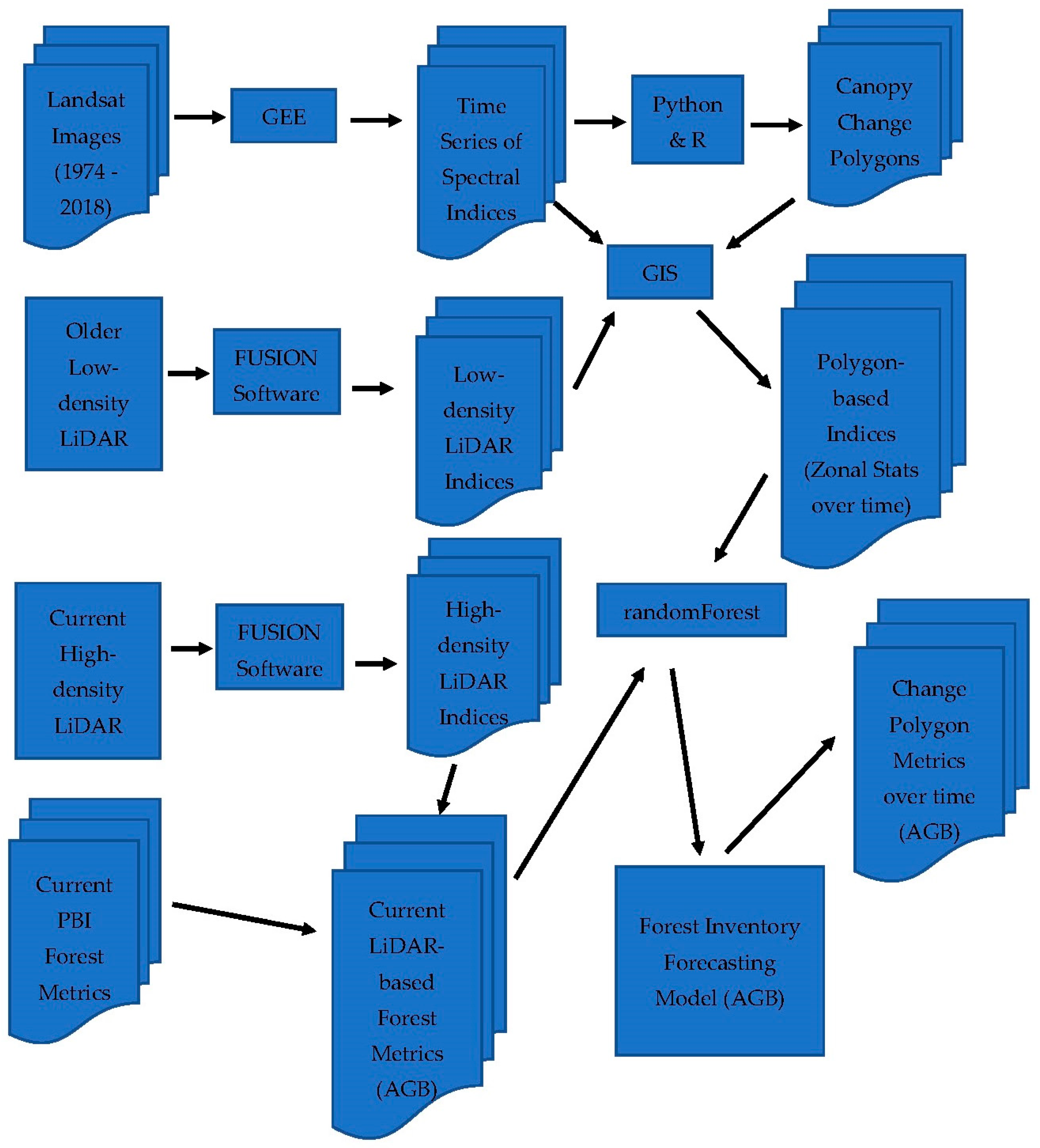
3] confirmed the utility of time-series Landsat spectral data in assessments of post-disturbance recovery from wildfire and harvest at the landscape level. Recent advances in the availability of moderately high-resolution satellite imagery coupled with the enhanced processing capabilities of super-computers or cloud platforms provides an opportunity to use broad-scale remote sensing approaches to detect forest canopy change and regeneration. Vogeler et al. [21,22] have detailed an approach utilizing the LandTrendr algorithm [1,23] on the Google Earth Engine (GEE) platform with 97.2% ± 1.9% validation accuracy for change vs. no change. This method maps forest canopy change (i.e., “change polygons”) at the landscape scale and estimates the timing and type of disturbances taking place between growing seasons (e.g., fast change). LandTrendr is based on the pixel-level trajectory of annual spectral reflectance values from forest canopies observed through Landsat time-series imagery collected during the peak growing seasons. The Minnesota Department of Natural Resources (MNDNR), Division of Forestry, Guideline Monitoring Program (GMP) has transitioned to using this method for harvest detection and site selection prior to field monitoring of the implementation of sustainable forest management practices. Although Vogeler et al. [22] report high user’s accuracies for disturbance agent classifications (80.0%, 89.6%, 89.7%, 90.2%, 92.9%, and 95.6% accuracy for wind, other disturbances (e.g., insect, disease, drought, or unspecified), flood, fire, conversion, and harvest, respectively), the GMP is currently assessing the spatial, temporal, and classification accuracy of this GEE approach to change detection via an independent use case related to timber harvest monitoring in Minnesota, USA. A raster version of these fast change data, covering 44 years from 1974 to 2018 with a minimum mapping unit of one hectare, can be found on the Minnesota Geospatial Commons website [24].
Increasing acquisitions of LiDAR, an advanced remote sensing technology able to accurately characterize forest structure, and recent advances in analytical capabilities have provided powerful means for assessing AGB in forested settings [25,26,27,
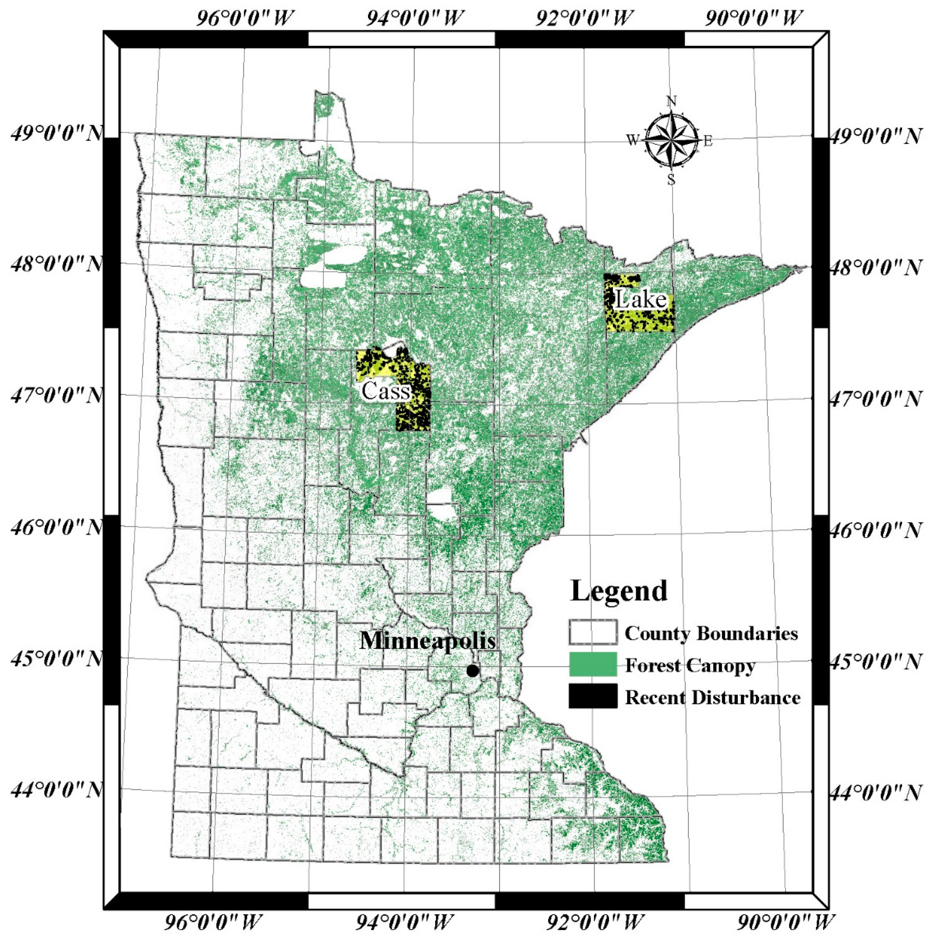
28]. The LiDAR-based forest inventory still requires sample plot measurements on the ground, and multi-temporal LiDAR collections can provide the basis for development of growth and yield models [28]. MNDNR initiated LiDAR acquisitions suitable for several natural resource applications in Minnesota in 2008. However, these initial statewide acquisitions were low point density and did not include a PBI component. High density LiDAR acquisitions paired with PBI for parts of Cass and Lake counties were initiated in 2017, enabling development of LiDAR-based inventory metrics for these areas, and providing LiDAR point cloud data for two points in time. These multi-temporal LiDAR datasets provide important baseline information across large landscapes and administrative areas. Implementation of the Minnesota LiDAR Plan has begun and, if successful, will result in acquisitions of high-density LiDAR statewide. This new statewide high-density LiDAR dataset paired with PBI fieldwork will enhance state forest inventories [29,30]. When combined with temporally referenced spectral indices, these data have the potential to provide important information related to forest composition, structure, growth, and productivity across substantial spatial extents (e.g., management units to ecological landscapes).
Here, we test the hypothesis that statewide low-density LiDAR acquired in Minnesota from 2008 to 2012 (circa 2010), paired with Landsat-derived spectral indices for growing seasons between 1974 and 2018 can be used in a modeling environment to create accurate estimates of standing biomass over time (past, present, and future) with ground truth referenced to AGB estimates derived from high-density LiDAR and PBI datasets acquired in 2017 and 2018 in Cass and Lake Counties. In doing so, we test the ability of satellite-derived spectral indices to supplement, augment, and correct for potential misinformation represented in older LiDAR acquisitions (resulting from ongoing disturbance and growth since time of acquisition). We also examine differential forest growth after canopy disturbance. Specifically, we test the null hypothesis that there is no significant difference in mean biomass accumulation over time among different disturbance agents on change polygons identified by Vogeler et al. [21]. This work combines and builds on multiple lines of inquiry related to forest inventory [3,28,31], remote sensing [1,3,21,22,23], and forecasting [28,31,32] methodology to illustrate a means of producing time series estimates of AGB for forested regions of the world where the necessary data resources exist.

2. Materials and Methods

2.1. Research Landscape and Data Preparation

The climate in Minnesota (north-central United States of America) is humid continental with summertime high temperatures averaging ~25 °C in the north and ~30 °C in the south with extremes as high as 46 °C. Winters in Minnesota are cold with average temperatures well below freezing (extremes may reach −51 °C). Average annual precipitation ranges from 890 mm in the southeast to 510 mm in the northwest with substantial snow accumulation during winter months. The average growing season ranges from 90 days in the north to 160 days in the southeast [33]. The glacial till plain landscapes in the study areas (Figure 1) are composed substantially of southern boreal forest and mixed hardwood forest (dense conifer and mixed conifer–deciduous), interspersed with significant numbers of wetlands and glacial lakes. Timber harvest, fires, windstorms, floods, insect infestations, and diseases continue to shape Minnesota’s forested landscape (Table 1).
The acquisition areas for two high density LiDAR pilot sites in Cass and Lake Counties (total about 600,000 hectares) in northern Minnesota (Figure 1) were selected as the areas of interest for this study. LiDAR-derived AGB was considered as the response variable, which is assumed to be related to regeneration of forest stands disturbed by various agents of change. The high-density LiDAR for Cass and Lake Counties, acquired during autumn 2017 and 2018 using different sensors, contained an average of 32 and 54 points per square meter, respectively. The results of LiDAR dependent inventory models including AGB are unpublished but reported to the Legislative Citizens Commission on Minnesota Resources [34]. The initial analysis for model accuracy is based on pixel/plot level comparisons of predictions and field observations.
The Landsat family of satellites has been collecting earth imagery continuously since 1974 using various sensors. Currently, Landsat 8 collects earth imagery at 15 m and 30 m resolutions with a 16-day repeat observation cycle. Current collections include 11 bands of visible, near-infrared, short-wave infrared, and thermal infrared light [35]. Recently, the full collection of Landsat data has become available for public use via the GEE cloud computing environment. We use this rich library of earth imagery to produce time-series of tasseled cap [36] brightness and greenness indices using cloud free season-averaged images (9–10 observations per growing season) for years between 1974 and 2018. These methods followed intermediate steps used by Vogeler et al. [21] employing the ee-LandsatLinkr [37] and LandTrendr [1,14] algorithms, available via GEE, to detect changed/disturbed areas (polygons), along with classification of change agents over time.
We used change polygons produced by the full process as test subjects for AGB modelling, incorporating both satellite-based spectral indices and LiDAR-derived information as predictive variables. Low-density LiDAR from Minnesota’s first ever statewide collect (circa 2010—hereafter called statewide 2010) was processed to produce a digital terrain model (DTM—ground surface returns), digital surface model (DSM—top of canopy returns), a canopy height model (CHM = DSM − DTM), and several other grid metrics (Table 2). Zonal statistics (mean, minimum, maximum, standard deviation, majority, etc.) derived from LiDAR and satellite imagery were then calculated for the change polygons and used as predictors in our AGB modelling effort (Table 2).

2.2. Data Analysis and Modelling Framework

Landsat time series and LiDAR-derived predictors (all LiDAR indices were derived using FUSION software [38]) were summarized within the boundary of each change polygon (minimum, maximum, mean, majority, standard deviation, coefficient of variation, and sum over time since disturbance) by running zonal statistics in a GIS environment to merge predictors with the corresponding polygon-level AGB for regression modeling (Supplementary Materials). The tasseled cap greenness index was also summarized over time for each polygon to provide a statistic closely related (R-squared = 0.86) to net CO2 uptake by the forest [39]. We also used the disturbance agent and year of change identified by Vogeler et al. [21] for change polygons as model predictors.
We considered two samples of the data (i.e., number of change polygons with minimum size of one hectare) for AGB modeling within the high-density LiDAR acquisition areas. These samples correspond to 7996 and 10,068 sites experiencing disturbance before 2011 and 2018, respectively.
In both samples, statewide 2010 LiDAR and time-series Landsat variables from 1974 to 2018 were used as predictors. One sample (79.4% of sites) represented all canopy disturbances prior to initial statewide LiDAR acquisition (circa 2010), while in the other sample, 20.6% experienced disturbance after the initial statewide LiDAR acquisition.
Because standing biomass is relevant to our understanding of site-level differences resulting from various disturbance agents, we examined this metric with additional detail. We used all available spatial predictors including high-density LiDAR and the full suite of spectral indices for the comparison of mean standing biomass across agent-wise disturbances for the time since disturbance (n = 10,068).
Time since disturbance was calculated annually for every change polygon as the difference between the date of disturbance and the appropriate date (year) of observation after disturbance (1974–2018 for Landsat indices, 2011 for the low-density LiDAR, and 2017 or 2018 for the high-density LiDAR). In total, changes in 31 unique predictor variables (Table 2) were considered across 44 years. All data were processed and assembled into a modeling data frame (Supplementary Data) using R [40]. The sum of accumulated greenness since time of disturbance was also summarized for each polygon using the dplyr package [41] from the tidyverse suite of data manipulation tools [42] in R.
The initial set of predictors was reduced using a variable selection process to identify and remove multi-collinear predictors. This selection process used a multivariate variable screening method based on QR-matrix decomposition [26]. Subsequently, a randomForest [43,44] (RF)-based model selection procedure was applied to obtain a parsimonious set of predictor variables. The set of predictors obtained from the RF model selection procedure was also subjected to forward and backward methods of stepwise regression [45] to identify statistically significant predictors.
The optimal sets of predictors were then used in the RF modeling framework. The RF method can estimate and rank the importance of predictors for each model. RF also gives an unbiased estimate of mean squared error through internal cross-validation and hence does not require a separate validation dataset. RF creates an ensemble of multiple regression tree models (for continuous variables), each constructed from a bootstrap subsample (about 66%) of the training data frame, and estimates model mean squared error (MSE) as the average value of the errors met with the out-of-bag data corresponding to approximately 33% of the plots that are withheld from the bootstrap subsample. Finally, AGB models were fit for each disturbance agent and for all agents combined. All RF models were created using a random subset of the data selected without replacement, selection of 2 random predictors to be removed from consideration at each branch of the “tree” (e.g., mtry), and a maximum of 501 trees generated for each model. See Figure 2 for a generalized overview of the full data management and model development process.
Finally, we examined potential relationships between disturbance agent and post-disturbance biomass accumulation rates. One necessary step to looking at biomass accumulation over time was to model initial biomass remaining at the time/year of disturbance, because the required formula for calculating net accumulation (e.g., growth − mortality) is (StandingBiomass − InitialBiomass)/Time. For estimation of initial AGB, we used the model and dataset from the RF modeling process using 7996 sites. The RF model was used to make predictions of initial biomass for the year of disturbance. Hence, data used to inform the estimate of initial biomass were selected from sites experiencing disturbance prior to the date of low-density LiDAR collection (i.e., 2010). We use the 5–15-year window following disturbance as a benchmark for biomass accumulation because initially high variability related to recruitment is more stable by 5 years. In addition, this date range provides a large enough sample to assess error from our estimate of biomass post-disturbance. In total, this means we have a chance to see the signal from biomass accumulation within this window. Average modeled AGB accumulation at various times following disturbance was graphed using a generalized additive (GAM) model within ggplot2 [46]. The term GAM is taken to include any quadratically penalized generalized linear model (GLM). The degree of smoothness is estimated as part of fitting. Smoothing terms are represented using regression splines with parameters selected by Restricted Maximum Likelihood (REML) [47]. Finally, we used a pairwise t-test to identify any significant differences in biomass accumulation following disturbance by different agents.

3. Results

Total forest cover in the two areas of interest (AOI) was 397,317 ha, with a total of 41,245 ha (11.46%) disturbed at least once over the period of observation (1974–2018). Only the most recent disturbances at any site were included in the 41,245 ha figure. Change polygons varied in shape and size between 1 and 234 ha with the average being 5 ha (SD = 7.1 ha). 
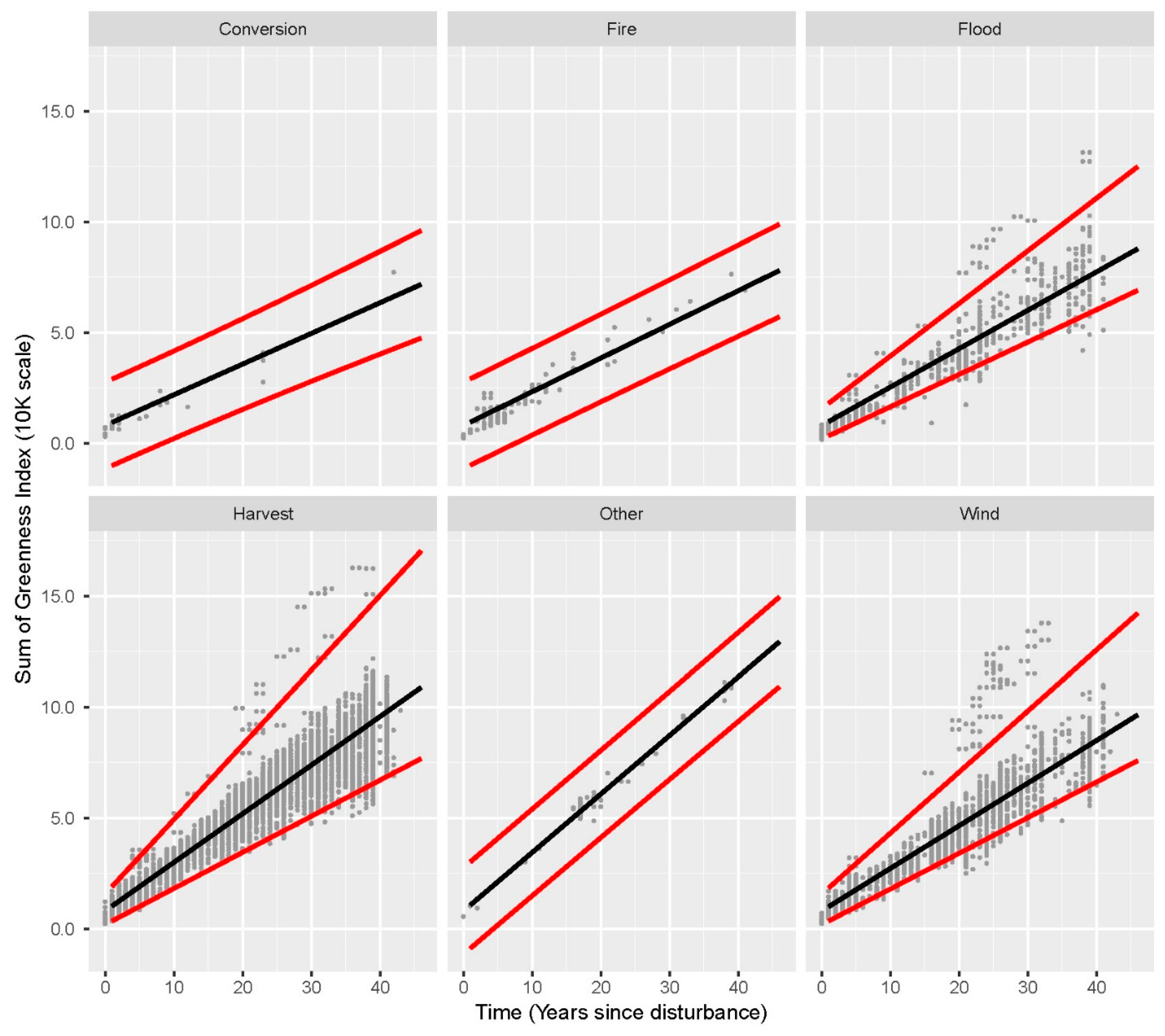
Figure 3 shows the relationship between time since disturbance and accumulated biophysical capacity for carbon dioxide uptake by the forest as captured by the tasseled cap greenness index over time [39].
Models predicting AGB, given spectral indices observed since disturbance, and intermediate low-density LiDAR information where applicable, are shown in Table 3. The amount of variance explained by each model and importance values (as percent increase in mean squared error when a predictor is removed) are also shown. The combined and agent-specific models could be reconstructed using each predictor containing an importance value in the column for a given model. These results are summarized for the modeling processes utilizing all sites, and using only sites disturbed prior to 2011.
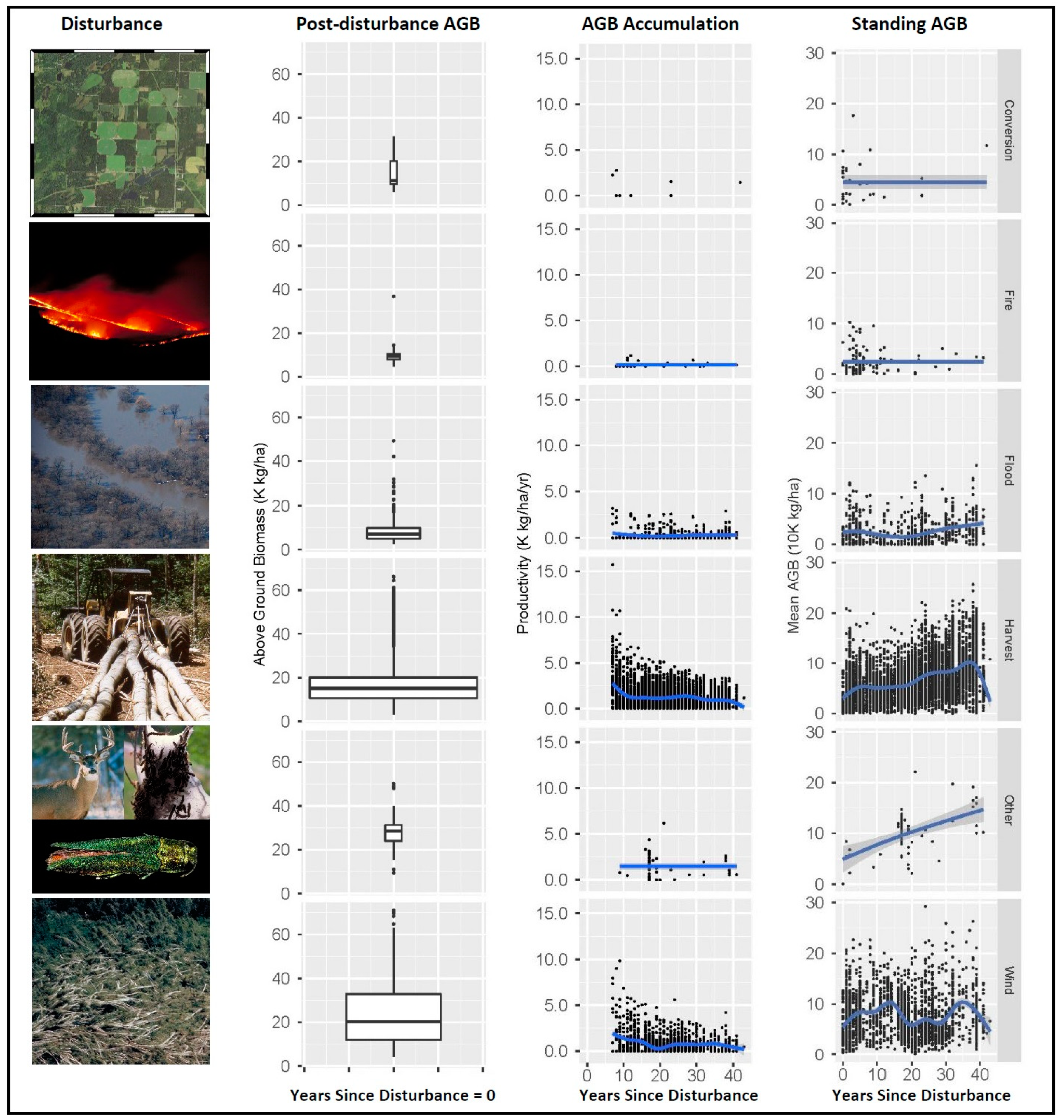
Standing AGB for sites experiencing different disturbance agents is shown in Table 4 and Figure 4. In Table 4, Time represents the average time since disturbance for observations corresponding to that agent of change. Time is related to the opportunity for regrowth of AGB following loss to fire, wind, harvest, or other factors. Further, differences in the average time since disturbance for various agents is an indication of the frequency with which these events tend to occur across the bio-regional landscape. An ANOVA for standing AGB using the full dataset indicated that there were significant differences in AGB predictions for different agents (p-value < 2.2 × 10⁻¹⁶) (Figure 4). A pairwise t-test (with Bonferroni adjustment) for the effect of inter-group variations showed that there were statistically significant differences (α = 0.05) between harvest and each other disturbance type, as well as between wind and conversion.
Non-significant comparisons included conversion and fire, conversion and flood, and fire and flood (Table 5). Statistics for estimates of productivity between 5 and 15 years after disturbance are shown in Table 6. A pairwise t-test (with Bonferroni adjustment) of between group differences in biomass accumulation over time showed that there was a statistically significant difference (α = 0.05) between harvest and fire, between harvest and flood, and between harvest and wind. Significant differences in biomass productivity over time also existed between fire and other, flood and other, wind and other, and between wind and flood (Table 7).

4. Discussion

Substantial research over many years has provided a firm basis for our understanding of forest growth and yield [48,49,50,51,52,53,54,55,56,57,58,59,60]. Although a full review of this research is beyond the scope of the current manuscript, it is important to note that our expectations related to development of AGB following disturbance are rooted in this body of literature.
Building on results from previous research comparing post-disturbance recovery from wildfire and harvest [3], we find clear differences in standing AGB and stand regeneration over time for different disturbance agents. Standing biomass and biomass accumulation rates indicate different things related to disturbance severity and recovery from disturbance. For example, wind and harvest disturbances often have more initial AGB relative to fire and flood. This may be an indication that prevailing disturbance intensity from wind and harvest are either less than that for fire and flood, or are more variable, with some sites retaining substantial AGB or established seedlings following disturbance. Indeed, groups of outliers observed for accumulated greenness associated with these disturbances (Figure 2) may be explained by the presence of advance regeneration retained after variable levels of disturbance. While White et al. [3] found higher variability in regrowth of forest canopy after wildfire compared to harvest, little research exists for comparison of differences in AGB development following the range of disturbances analyzed here.
Our comparison of differences in standing biomass among disturbance agents yielded clear and significant results. This observation is an indicator that something different is happening on sites experiencing different types of disturbance in the years following the event and corresponds closely to the conclusions of White et al. [3]. Such differences are expected to be cumulative over time, and to become more apparent as time goes on. Senf and Seidl [10] use Landsat time series to assess forest canopy disturbance and recovery across Europe, but do not directly address the issue of AGB development. However, mirroring the conclusions of White et al. [3], Senf and Seidl [10] point to fire disturbance as a factor leading to slower canopy recovery. Research using tree ring analysis to examine carbon storage, sequestration, and biodiversity on a longer timescale [17] also found that the highest rates of carbon sequestration occurred on more recently disturbed plots. Our results agree with these findings and suggest that sustainable timber harvest at levels below the regional annual increment, and adjusted for natural disturbance, may contribute to greater forest resiliency. AGB productivity following harvest is significantly different from (greater than) that observed for wind, flood, and fire disturbance agents. Collectively, these observations may have significant and substantial meaning for efforts to sequester carbon from the atmosphere via forest management.
Biomass accumulation (an indicator of productivity) is the response of trees remaining or growing onto a site following a disturbance. Established research leads to the expectation that, initially, this response will be quite strong, but will moderate as competition effects come into play following establishment of a cohort, e.g., saturation of the newly available growing space. Initial AGB remaining after a disturbance will influence the path this development takes. Indeed, the general trend of reduced biomass accumulation with time since disturbance is both clearly apparent and expected in our results [16,17]. Harvest appears to result in the largest and most consistent productivity response to disturbance, with harvested sites experiencing roughly six times the rate of biomass accumulation seen for sites subjected to stand replacing fire or flood (years 5–15 post disturbance), and a nearly 20% increase in productivity when compared to sites subjected to wind-caused canopy loss.
Essentially, our results indicate that harvest not only resets the accumulation rate of biomass (productivity) to a higher level than other disturbance types but often leads to the accumulation of larger biomass loads (standing biomass) with time. These observations may be explained by intentional silvicultural strategies employed in conjunction with timber harvest (e.g., seed tree retention, artificial regeneration/planting, site preparation, and selection of high-quality sites with potential for rapid natural regeneration) or represent a response to the large increase in available growing space and minimal disturbance of the ground layer frequently resulting from these disturbances. When combined with the potential for mid-term storage of carbon in timber products used for construction (housing, commercial, and other structures) [61,62,63] or carbon offsets associated with biomass energy production [64], this higher level of biomass production means that forest management for timber and other uses can be a helpful tool for carbon sequestration in the effort to mitigate anthropogenic climate change.
Because our estimates of initial AGB are modelled, results should be taken as a general understanding of regrowth following disturbance, not as an absolute truth. However, our independent test for 54 harvests monitored by GMP explained 90.09% of variance, indicating good correspondence of the model to observations. It is also understood that LiDAR data serve as a snapshot in time and do not represent true conditions before or after the data are collected. This depreciation of information relevance is clearly mitigated to a large degree using Landsat spectral indices available over long time periods. Error involved with estimates of initial and standing AGB presented here results from imprecise minimum mapping units for disturbance (1 ha) and inherent variability in the severity of discrete disturbance events. This model related error inflates the expected variance for our estimates of biomass accumulation, thereby complicating interpretation of the results. Another source of variability in our initial AGB estimates comes from the estimate of disturbance dates derived from change detection. Inaccuracies of 1–3 years are common in the change detection dates and influence our estimates of initial AGB following disturbance. Further, error associated with disturbance agent classification also increases our uncertainty regarding initial AGB. Nonetheless, clear differences exist in forest regeneration rate and character between sites disturbed by different agents of change. These differences result in varying rates of biomass accumulation over time and differences in standing stocks of biomass on sites affected by various agents of change. These differences are thought to be related to disturbance severity, species level responses, canopy structure development, community compositions, and carbon sequestration and storage potentials resulting from distinct disturbance types.
We have also shown that older low-density LiDAR data can serve as a good predictor in models producing AGB estimates for forested regions of interest. The information provided by these low-density LiDAR-derived products can be effectively leveraged with the addition of widely available spectral indices derived from satellite sensors, and more current high-density LiDAR paired with PBI within portions of the region of interest. The combination of different platforms and vintages of remotely sensed data products can serve to inform and model landscape-scale changes over time and continues to enhance the utility of older geospatial datasets, further extending their return on investment. These observations may also benefit canopy change detection efforts used for monitoring of timber harvest and other disturbances.

5. Conclusions

We have tested the hypothesis that older low-density LiDAR, paired with Landsat-derived spectral indices available over a long time-period can be used in a modeling environment to create accurate estimates of standing biomass. Comparison of our modelling results against ground truth referenced to AGB estimates derived from high-density LiDAR and PBI datasets yielded good correlation between modelled estimates and observed values (R-squared ~0.85). In testing our primary hypothesis, we have shown that satellite-derived spectral indices are able to supplement, augment, and correct for potential misinformation present in older LiDAR acquisitions quite effectively.
Low-density LiDAR data provide important information related to existing levels of AGB in a forested setting. This observation is especially relevant when canopy height data are paired with indices of wetness and greenness derived from satellite imagery over time. In combination, low-density LiDAR and spectral indices can be used to accurately predict current AGB, as determined from high density LiDAR and PBI reference data. High-density LiDAR data provide a range of useful information for development of predictive models of AGB across a broader region and serve as important benchmarks for monitoring over time.
We also examined differential forest growth after canopy disturbance and have rejected the null hypothesis that there is no significant difference in standing biomass or mean biomass accumulation over time among different disturbance agents. Over time, the response to disturbance by various agents of change results in clear differences in AGB. Results presented here indicate profound differences in recruitment and forest development following various events resulting in canopy change. This research provides quantifiable clarity, adding to our understanding that forest management via timber harvest can be used as an effective tool to increase AGB productivity.
Periodic re-measurement with high and low-density LiDAR would further contribute to our understanding of differences in forest regrowth following disturbance by providing a more solid baseline (e.g., multiple observations over time) related to changes in AGB and tightening resulting confidence intervals for the kinds of models used here. However, high quality LiDAR data are expensive to collect over large areas, so additional analysis of the benefits of using methods described here to model landscape-scale AGB over time should be completed. Such analyses would inform the needed re-measurement interval, help target areas of interest where they are most relevant to improving model accuracy, and provide quantifiable information related to return on investment for such data acquisition. This research also identifies some areas of uncertainty stemming from the change detection methods used, and further research into this important field of study is merited. The combination of multi-temporal LiDAR-derived and satellite-based spectral indices may provide another avenue for improving canopy change detection methods and our understanding of forest recovery following disturbance.

Supplementary Materials

The following are available online at https://www.mdpi.com/article/10.3390/earth3010006/s1, Table S1: Research and modelling data for regeneration following disturbance in Minnesota, USA.

Author Contributions

Conceptualization: D.C.W. and J.C.; Formal analysis, R.K.D.; Funding acquisition, D.C.W. and J.C.; Methodology, D.C.W. and R.K.D.; Project administration, D.C.W.; Validation, R.K.D.; Visualization, D.C.W.; Writing—original draft, D.C.W. and R.K.D.; Writing—review and editing, D.C.W., R.K.D., and J.C. All authors have read and agreed to the published version of the manuscript.

Funding

All funding for this research was provided by the Lessard-Sams Outdoor Heritage Council Clean Water Fund through the Guideline Monitoring Program (Minnesota Department of Natural Resources—Division of Forestry). Matching funds for project coordination and manuscript development were also provided by the Minnesota Department of Natural Resources—Division of Forestry—Resource Assessment.

Institutional Review Board Statement

Not applicable.

Informed Consent Statement

Not applicable.

Data Availability Statement

See Supplementary Materials. Additional data available upon request from the authors.

Conflicts of Interest

The authors declare no conflict of interest. The funders had no role in the design of the study; in the collection, analyses, or interpretation of data; in the writing of the manuscript; or in the decision to publish the results.

References

  1. Kennedy, R.E.; Yang, Z.; Cohen, W.B. Detecting trends in forest disturbance and recovery using yearly Landsat time series: 1. LandTrendr—Temporal segmentation algorithms. Remote. Sens. Environ. 2010, 114, 2897–2910. [Google Scholar] [CrossRef]
  2. Bartels, S.F.; Chen, H.Y.H.; Wulder, M.A.; White, J.C. Trends in post-disturbance recovery rates of Canada’s forests following wildfire and harvest. For. Ecol. Manag. 2016, 361, 194–207. [Google Scholar] [CrossRef] [Green Version]
  3. White, J.C.; Wulder, M.A.; Hermosilla, T.; Coops, N.C.; Hobart, G.W. A nationwide annual characterization of 25 years of forest disturbance and recovery for Canada using Landsat time series. Remote Sens. Environ. 2017, 194, 303–321. [Google Scholar] [CrossRef]
  4. White, J.C.; Saarinen, N.; Wulder, M.A.; Kankare, V.; Hermosilla, T.; Coops, N.C.; Holopainen, M.; Hyyppä, J.; Vastaranta, M. Assessing spectral measures of post-harvest forest recovery with field plot data. Int. J. Appl. Earth Obs. Geoinf. 2019, 80, 102–114. [Google Scholar] [CrossRef]
  5. Frolking, S.; Palace, M.W.; Clark, D.B.; Chambers, J.Q.; Shugart, H.H.; Hurtt, G.C. Forest disturbance and recovery: A general review in the context of spaceborne remote sensing of impacts on aboveground biomass and canopy structure. J. Geophys. Res. 2009, 114, G00E02. [Google Scholar] [CrossRef]
  6. Chazdon, R.L.; Brancalion, P.H.S.; Laestadius, L.; Bennett-Curry, A.; Buckingham, K.; Kumar, C.; Moll-Rocek, J.; Guimarães Vieira, I.C.; Wilson, S.J. When is a forest a forest? Forest concepts and definitions in the error of forest and landscape restoration. Ambio 2016, 45, 538–550. [Google Scholar] [CrossRef] [PubMed]
  7. Meli, P.; Holl, K.D.; Benayas, J.M.R.; Jones, H.P.; Jones, P.C.; Montoya, D.; Mateos, D.M. A global review of past land use, climate, and active vs. passive restoration effects on forest recovery. PLoS ONE 2017, 12, e0171368. [Google Scholar] [CrossRef]
  8. Wise, L.; Marland, E.; Marland, G.; Hoyle, J.; Kowalczyk, T.; Ruseva, T.; Colby, J.; Kinlaw, T. Optimizing sequestered carbon in forest offset programs: Balancing accounting stringency and participation. Carbon Balance Manag. 2019, 14, 16. [Google Scholar] [CrossRef]
  9. Frazier, R.J.; Coops, N.C.; Wulder, M.A. Boreal Shield Forest disturbance and recovery trends using Landsat time series. Remote Sens. Environ. 2015, 170, 317–327. [Google Scholar] [CrossRef]
  10. Senf, C.; Seidl, R. Post-disturbance canopy recovery and the resilience of Europe’s forests. Glob. Ecol. Biogeogr. 2021, 31, 25–36. [Google Scholar] [CrossRef]
  11. Alves, L.F.; Vieira, S.A.; Scaranello, M.A.; Camargo, P.B.; Santos, F.A.M.; Joly, C.A.; Martinelli, L.A. Forest structure and live aboveground biomass variation along an elevational gradient of tropical Atlantic moist forest (Brazil). For. Ecol. Manag. 2010, 260, 679–691. [Google Scholar] [CrossRef]
  12. Soriano-Luna, M.D.Á.; Ángeles-Pérez, G.; Guevara, M.; Birdsey, R.; Pan, Y.; Vaquera-Huerta, H.; Valdez-Lazalde, J.R.; Johnson, K.D.; Vargas, R. Determinants of above-ground biomass and its spatial variability in a temperate forest managed for timber production. Forests 2018, 9, 490. [Google Scholar] [CrossRef] [Green Version]
  13. Urbazaev, M.; Thiel, C.; Cremer, F.; Dubayah, R.; Migliavacca, M.; Reichstein, M.; Schmullius, C. Estimation of forest aboveground biomass and uncertainties by integration of field measurements, airborne LiDAR, and SAR and optical satellite data in Mexico. Carbon Balance Manag. 2018, 13, 5. [Google Scholar] [CrossRef] [Green Version]
  14. Anderson-Teixeira, K.J.; Miller, A.D.; Mohan, J.E.; Hudiburg, T.W.; Duval, B.D.; DeLucia, E.H. Altered dynamics of forest recovery under a changing climate. Glob. Chang. Biol. 2013, 17, 2001–2021. [Google Scholar] [CrossRef]
  15. Orusa, T.; Borgogno Mondino, E. Exploring Short-term climate change effects on rangelands and broad-leaved forests by free satellite data in Aosta Valley (Northwest Italy). Climate 2021, 9, 47. [Google Scholar] [CrossRef]
  16. McMahon, S.M.; Parker, G.G.; Miller, D.R. Evidence for a recent increase in forest growth. Proc. Natl. Acad. Sci. USA 2010, 107, 3611–3615. [Google Scholar] [CrossRef] [Green Version]
  17. Mikoláš, M.; Svitok, M.; Bače, R.; Meigs, G.W.; Keeton, W.S.; Keith, H.; Buechling, A.; Trotsiuk, V.; Kozák, D.; Bollmann, K.; et al. Natural disturbance impacts on trade-offs and co-benefits of forest biodiversity and carbon. Proc. R. Soc. B 2021, 288, 20211631. [Google Scholar] [CrossRef] [PubMed]
  18. Wilson, D.C.; Morin, R.S.; Frelich, L.E.; Ek, A.R. Monitoring disturbance intervals in forests: A case study of increasing forest disturbance in Minnesota. Ann. For. Sci. 2019, 76, 78. [Google Scholar] [CrossRef]
  19. Millar, C.I.; Stephenson, N.L. Temperate forest health in an era of emerging megadisturbance. Science 2015, 349, 823–826. [Google Scholar] [CrossRef]
  20. Stevens-Rumann, C.S.; Kemp, K.B.; Higuera, P.E.; Harvey, B.J.; Rother, M.T.; Donato, D.C.; Morgan, P. and Veblen, T.T. Evidence for declining forest resilience to wildfires under climate change. Ecol. Lett. 2018, 21, 243–252. [Google Scholar] [CrossRef] [PubMed]
  21. Vogeler, J.C.; Braaten, J.D.; Slesak, R.A.; Falkowski, M.J. Extracting the full value of the Landsat archive: Inter-sensor harmonization for the mapping of Minnesota forest canopy cover (1973–2015). Remote Sens. Environ. 2018, 209, 363–374. [Google Scholar] [CrossRef]
  22. Vogeler, J.C.; Slesak, R.A.; Fekety, P.A.; Falkowski, M.J. Characterizing over four decades of forest disturbance in Minnesota, USA. Forests 2020, 11, 362. [Google Scholar] [CrossRef] [Green Version]
  23. Kennedy, R.E.; Yang, Z.; Gorelick, N.; Braaten, J.; Cavalcante, L.; Cohen, W.B.; Healey, S. Implementation of the LandTrendr algorithm on google earth engine. Remote Sens. 2018, 10, 691. [Google Scholar] [CrossRef] [Green Version]
  24. Minnesota Department of Natural Resources. Most Recent Fast Forest Disturbances in Minnesota Version 4.0. 2019. Available online: https://gisdata.mn.gov/dataset/env-fast-forest-disturbances (accessed on 30 December 2021).
  25. Deo, R.K.; Russell, M.B.; Domke, G.M.; Woodall, C.W.; Falkowski, M.J.; Cohen, W.B. Using Landsat time-series and LiDAR to inform aboveground biomass baselines in northern Minnesota, USA. Can. J. Remote Sens. 2017, 43, 28–47. [Google Scholar] [CrossRef]
  26. Deo, R.K.; Russell, M.B.; Domke, G.M.; Woodall, C.W.; Andersen, H.E.; Cohen, W.B. Evaluating site-specific and generalized spatial models of aboveground forest biomass based on Landsat time-series and LiDAR strip samples in the Eastern USA. Remote Sens. 2017, 9, 598. [Google Scholar] [CrossRef] [Green Version]
  27. Deo, R.K.; Froese, R.E.; Falkowski, M.J.; Hudak, A.T. Optimizing variable radius plot size and LiDAR resolution to model standing volume in conifer forests. Can. J. Remote Sens. 2016, 42, 428–442. [Google Scholar] [CrossRef]
  28. Tompalski, P.; Coops, N.C.; White, J.C.; Goodbody, T.R.; Hennigar, C.R.; Wulder, M.A.; Socha, J.; Woods, M.E. Estimating changes in forest attributes and enhancing growth projections: A review of existing approaches and future directions using airborne 3D point cloud data. Curr. For. Rep. 2021, 7, 1–24. [Google Scholar] [CrossRef]
  29. Minnesota Geospatial Advisory Council. Minnesota Lidar Plan. 2021. Available online: https://www.mngeo.state.mn.us/committee/3dgeo/acquisition/Minnesota_Lidar_Plan.pdf (accessed on 30 December 2021).
  30. Sugarbaker, L.J.; Eldridge, D.F.; Jason, A.L.; Lukas, V.; Saghy, D.L.; Stoker, J.M.; Thunen, D.R. Status of the 3D Elevation Program, 2015; Open-File Report 2016-1196; US Geological Survey: Reston, VA, USA, 2017; 13p. [Google Scholar] [CrossRef] [Green Version]
  31. Wahlenberg, W.G. Methods of Forecasting Timber Growth in Irregular Stands; Technical Bulletin 1941, 796; U.S. Department of Agriculture, Southern Forest Experiment Station, Forest Service. Available online: https://naldc.nal.usda.gov/download/CAT86200791/PDF (accessed on 21 December 2021).
  32. Lamb, S.M.; MacLean, D.A.; Hennigar, C.R.; Pitt, D.G. Forecasting forest inventory using imputed tree lists for LiDAR grid cells and a tree-list growth model. Forests 2018, 9, 167. [Google Scholar] [CrossRef] [Green Version]
  33. Minnesota Department of Natural Resources. Minnesota Climate Summaries and Publications. Available online: https://www.dnr.state.mn.us/climate/summaries_and_publications/index.html (accessed on 30 December 2021).
  34. Legislative Citizens Commission on Minnesota Resources. Project Report: Development of Innovative Cost-Saving Methodology for Forest Inventory 2016. Available online: https://www.lccmr.leg.mn/projects/2016/finals/2016_03o.pdf (accessed on 30 December 2021).
  35. United States Geological Survey. Landsat 8. Available online: https://www.usgs.gov/landsat-missions/landsat-8 (accessed on 30 December 2021).
  36. Ali Baig, M.H.; Zhang, L.; Shuai, T.; Tong, Q. Derivation of a tasselled cap transformation based on Landsat 8 at-satellite reflectance. Remote. Sens. Lett. 2014, 5, 423–431. [Google Scholar] [CrossRef]
  37. Braaten, J.; Cohen, W.; Yang, Z. LandsatLinkr: An Automated System for Processing Large Volumes of Landsat Imagery and Building Long Spectrally Consistent Chronologies across MSS, TM, ETM+, and OLI Sensors; Laboratory for Applications of Remote Sensing in Ecology, Oregon State University: Corvallis, OR, USA, 2021; Available online: http://jdbcode.github.io/LandsatLinkr/index.html (accessed on 27 December 2021).
  38. McGaughey, R.J. FUSION/LDV LIDAR Analysis and Visualization Software. USDA Forest Service, Pacific Northwest Research Station. Available online: http://forsys.cfr.washington.edu/FUSION/fusion_overview.html (accessed on 3 January 2022).
  39. McMillan, A.M.S.; Goulden, M.L. Age-dependent variation in the biophysical properties of boreal forests. Glob. Biogeochem. Cycles 2008, 22, GB2019. [Google Scholar] [CrossRef]
  40. R Core Team. R: A Language and Environment for Statistical Computing; R Foundation for Statistical Computing: Vienna, Austria, 2019; Available online: https://www.R-project.org/ (accessed on 21 December 2021).
  41. Wickham, H.; François, R.; Henry, L.; Müller, K. dplyr: A Grammar of Data Manipulation. R Package Version 0.8.3. 2019. Available online: https://CRAN.R-project.org/package=dplyr (accessed on 21 December 2021).
  42. Wickham, H.; Averick, M.; Bryan, J.; Chang, W.; McGowan, L.D.; François, R.; Grolemund, G.; Hayes, A.; Henry, L.; Hester, J.; et al. Welcome to the tidyverse. J. Open Source Softw. 2019, 4, 1686. [Google Scholar] [CrossRef]
  43. Breiman, L. Random forests. Mach. Learn. 2001, 45, 5–32. [Google Scholar] [CrossRef] [Green Version]
  44. Liaw, A.; Wiener, M. Classification and Regression by random Forest. R News 2002, 2, 18–22. [Google Scholar]
  45. Hocking, R.R. A Biometrics Invited Paper. The analysis and selection of variables in linear regression. Biometrics 1976, 32, 1–49. [Google Scholar] [CrossRef]
  46. Wickham, H. ggplot2: Elegant Graphics for Data Analysis; Springer: New York, NY, USA, 2016. [Google Scholar]
  47. Hastie, T.; Tibshirani, R. Generalized additive models. Stat. Sci. 1986, 1, 297–318. Available online: https://web.stanford.edu/~hastie/Papers/gam.pdf (accessed on 21 December 2021). [CrossRef]
  48. Brown, R.M.; Gevorkiantz, S.R. Revised. Volume, yield, and stand tables for tree species in the Lake States. Univ. Minn. Agric. Exp. Sta. Tech. Bull. 1934, 39, 208. [Google Scholar]
  49. Gevorkiantz, S.R.; Duerr, W.A. Methods of Predicting Growth of Forest Stands in the Forest Survey of the Lake States; USDA For. Serv. Lake States For. Exp. Stn. Econ. Notes; USDA Forest Service: Washington, DC, USA, 1938; Volume 9, p. 59.
  50. Buckman, R.E. Growth and Yield of Red Pine in Minnesota; USDA Forest Serv. Tech. Bull.; USDA Forest Service: Washington, DC, USA, 1962; 50p.
  51. Clutter, J.L. Compatible growth and yield models for loblolly pine. For. Sci. 1963, 9, 354–371. [Google Scholar]
  52. Schlagel, B.F. Growth and Yield of Quaking Aspen in North Central Minnesota; RP NC-58; USDA Forest Service: Washington, DC, USA, 1971; 11p.
  53. Sullivan, A.D.; Clutter, J.L. A simultaneous growth and yield for loblolly pine. For. Sci. 1972, 18, 76–86. [Google Scholar]
  54. Lundgren, A.L. The Effect of Initial Number of Trees per Acre and Thinning Densities on Timber Yields from Red Pine Plantations in the Lake States; RP NC-193; USDA Forest Service: Washington, DC, USA, 1981; 25p.
  55. Hahn, J.T.; Raile, G.K. Empirical Yield Tables for Minnesota; GTR NC-71; USDA Forest Service: Washington, DC, USA, 1982; 212p.
  56. Burkhart, H.E.; Sprinz, P.T. Compatible cubic volume and basal area projection equations for thinned old-field loblolly pine plantations. For. Sci. 1984, 30, 86–93. [Google Scholar]
  57. McDill, M.E.; Amateis, R.L. Measuring forest site quality using the parameters of a dimensionally compatible height growth function. For. Sci. 1992, 38, 409–429. [Google Scholar]
  58. Walters, D.K.; Ek, A.R. Whole stand yield and density equations for fourteen forest types in Minnesota. N. J. Appl. For. 1993, 10, 75–86. [Google Scholar] [CrossRef]
  59. Burkhart, H.E.; Tomé, M. Modeling Forest Trees and Stands; Springer: New York, NY, USA, 2012; 457p. [Google Scholar]
  60. Wilson, D.C.; Ek, A.R. Revised. Whole Stand Growth and Yield Models for Major Forest Types in the Upper Great Lakes Region; Staff Paper Series 254; Dept. of Forest Resources; University of Minnesota: St. Paul, MN, USA, 2019; 32p, (plus appendices); Available online: https://www.forestry.umn.edu/our-department/publications/ (accessed on 21 December 2021).
  61. Skog, K.E.; Nicholson, G.A. Carbon sequestration in wood and paper products. In The Impact of Climate Change on America’s Forests: A Technical Document Supporting the 2000 USDA Forest Service RPA Assessment; Joyce, L.A., Birdsey, R., Eds.; Gen. Tech. Rep. 2000; RMRS-GTR-59; Department of Agriculture, Forest Service, Rocky Mountain Research Station: Fort Collins, CO, USA, 2000; pp. 79–88. [Google Scholar]
  62. Skog, K.E. Sequestration of carbon in harvested wood products for the United States. For. Prod. J. 2008, 58, 56–72. [Google Scholar]
  63. Loehle, C. Carbon sequestration due to commercial forestry: An equilibrium analysis. For. Prod. J. 2020, 70, 60–63. [Google Scholar] [CrossRef]
  64. Kukrety, S.; Wilson, D.C.; D’Amato, A.W.; Becker, D.R. Assessing sustainable forest biomass potential and bioenergy implications for the northern Lake States region, USA. Biomass Bioenergy 2015, 81, 167–176. [Google Scholar] [CrossRef] [Green Version]
Figure 1. Cass and Lake County Minnesota study sites (yellow) with statewide forest canopy (green) and disturbed areas (black). Coordinate system: North American Datum of 1983, Universal Transverse Mercator Zone 15 North. For reference, 1 degree is equivalent to approximately 110 km in the north to south direction, or 78 km in the east to west direction.
Earth 03 00006 g001
Figure 2. Flowchart of data management and model development process.
Earth 03 00006 g002
Figure 3. Fitted (black line) and observed (gray dots) accumulated greenness index values over time since disturbance for the six agents of change. Red lines represent 95% confidence intervals around the fitted values. Greenness informs approximately 86% of observed variance in CO2 flux capacity within the forest [39].
Earth 03 00006 g003
Figure 4. Summary of initial above ground biomass following different disturbances, subsequent AGB accumulation rates, and standing AGB over time. Image credits: MNDNR, USGS.
Earth 03 00006 g004
Table 1. Area disturbed (hectares) within the study area (Figure 1) displayed by year of disturbance (1975–2017) and disturbance agent. This table includes areas corresponding to overlapping disturbances where more than one change event has occurred.
YearConversionFireFloodHarvestOtherWindTotal
19752.61--6.57-2.5211.7
1976--10.8954.54-11.777.1
1977-1.0811.3443223.6752.2520.3
1978--81.36879.874.2340.681006.1
1979-11.07123.571330.686.03374.311845.7
19804.05-100.71260.35-7.47372.6
1981--83.24506.76-17.1607.1
1982--5.94325.26-17.37348.6
1983--15.66400.11-38.07453.8
1984--4.3296.95--101.3
1985-2.07125.312052.885.4183.62369.3
19866.4615.0350.85676.92-39.96789.2
19877.021.26154.81785.24-291.012239.3
1988--26.19606.51-79.11711.8
1989-9.2712.03935.97-225.541182.8
1990--10.981044.521.17291.051347.7
19911.251.833.212203.681.08387.062628.1
1992--71.46896.04-180.771148.3
1993--53.73892.68-232.751179.2
19945.58-199.981654.213.06550.52413.3
1995--103.13979.2-78.941161.3
1996-7.7432.131007.001.0875.031123.0
1997-2.34593.511497.26-391.032484.1
1998--221.951531.1712.54162.421928.1
1999--87.931528.4418.27831.022465.7
200026.82-139.41782.7146.26355.821351.0
20012.5211.79102.421416.4689.46697.522320.2
20021.083.7897.38668.49-168.57939.3
2003--232.2591.33-39.42863.0
20041.891.8942.57733.4-450.481230.2
20052.521.4457.74969.21-124.21155.1
20062.8813.574.52578.56-73.71743.2
20074.2317.7366.69814.593.15233.21139.6
2008-16.4720.381096.24-140.191273.3
20095.9451.72110.971567.995.58287.552029.8
201031.9524.7550.581077.25-69.751254.3
2011-4.7723.22450.26-20.07498.3
201230.18383.49423.091571.16-756.243164.2
2013-117.54340.171104.55-250.551812.8
20144.05121.5177.2834.22-134.721271.7
201531.32123.21292.531919.084.86251.232622.2
201616.7518.6327.41714.848.821342.412128.9
2017--2.6117.91-8.5529.1
Total189.1963.94495.340,493.1234.79965.456,341.4
Table 2. Descriptions for spectral indices and LiDAR data used as predictors in models of above ground biomass.
Index (Predictor)Description (with Reference to Individual Change Polygons)
cvTCWCoefficient of variation for tasseled cap wetness values (of all 30-m pixels)
majorityTCGMajority of tasseled cap greenness values (of all 30-m pixels)
maxTCGMaximum of tasseled cap greenness values (of all 30-m pixels)
maxTCWMaximum of tasseled cap wetness values (of all 30-m pixels)
meanTCWMean of tasseled cap wetness values (of all 30-m pixels)
minTCGMinimum of tasseled cap greenness values (of all 30-m pixels)
minTCWMinimum of tasseled cap wetness values (of all 30-m pixels)
stdTCGStandard deviation of tasseled cap greenness values (of all 30-m pixels)
stdTCWStandard deviation of tasseled cap wetness values (of all 30-m pixels)
SumGreenSum of mean tasseled cap greenness index since time of disturbance (of all 30-m pixels)
maxElevAv_LowDensityMaximum of average elevations (of 20-m statewide LiDAR grids/pixels)
maxElevMax_LowDensityMaximum of maximum elevations (of 20-m statewide LiDAR grids/pixels)
maxElevP50_LowDensityMaximum of 50th percentile elevations (of 20-m statewide LiDAR grids/pixels)
maxPcCOV_LowDensityMaximum of percent cover (of 20-m statewide LiDAR grids/pixels)
meanElevAv_LowDensityMean of average elevations (of 20-m statewide LiDAR grids/pixels)
meanElevMax_LowDensityMean of maximum elevations (of 20-m statewide LiDAR grids/pixels)
meanElevP50_LowDensityMean of 50th percentile elevations (of 20-m statewide LiDAR grids/pixels)
meanPcCOV_LowDensityMean of percent cover (of 20-m statewide LiDAR grids/pixels)
minElevAv_LowDensityMinimum of average elevations (of 20-m statewide LiDAR grids/pixels)
minElevMax_LowDensityMinimum of maximum elevations (of 20-m statewide LiDAR grids/pixels)
minElevP50_LowDensityMinimum of 50th percentile elevations (of 20-m statewide LiDAR grids/pixels)
minPcCOV_LowDensityMinimum of percent cover (of 20-m statewide LiDAR grids/pixels)
stdElevAv_LowDensityStandard deviation of average elevations (of 20-m statewide LiDAR grids/pixels)
stdElevMax_LowDensityStandard deviation of maximum elevations (of 20-m statewide LiDAR grids/pixels)
stdElevP50_LowDensityStandard deviation of 50th percentile elevations (of 20-m statewide LiDAR grids/pixels)
stdPcCOV_LowDensityStandard deviation of percent cover (of 20-m statewide LiDAR grids/pixels)
timeCount in years since disturbance
Table 3. Percent increase in mean squared error when predictor is removed (RF) for agent specific and combined above ground biomass models.
PredictorAll *Pre-2011FireFloodHarvestOtherWind
cvTCW0.6----1.07-
majorityTCG1.131.1--0.75-0.81
maxTCG1.331.13-0.280.630.040.75
maxTCW1.810.87--0.720.250.97
meanTCW-2.12--1.91-1.26
minTCG-1.7-0.141.070.231.32
minTCW-1.17--1.040.45-
stdTCG--0.14--0.72-
stdTCW-----0.81-
SumGreen4.212.89-0.482.27-1.48
maxElevAv_LowDensity---0.71-2.56-
maxElevMax_LowDensity--0.27--2.31-
maxElevP50_LowDensity--0.54----
maxPcCOV_LowDensity--0.15--0.85-
meanElevAv_LowDensity12.116.520.882.5513.792.3913.46
meanElevMax_LowDensity8.8410.480.262.5610.11-5.69
meanElevP50_LowDensity---1.35-1.429
meanPcCOV_LowDensity--0.281.37---
minElevAv_LowDensity--0.4--2.25-
minElevMax_LowDensity-----3.35-
minElevP50_LowDensity2.33-0.46--0.39-
minPcCOV_LowDensity-----1.48-
stdElevAv_LowDensity--0.320.67-0.15-
stdElevMax_LowDensity---0.27-0.690.66
stdElevP50_LowDensity2.25-0.43--0.18-
stdPcCOV_LowDensity---0.32---
time3.542.1-0.251.511.281.46
Sample Size10,0687996315575563551781
% Variance Explained85.14 **87.5451.774.586.6166.6886.37
* Combined AGB model produced using all available data. ** An independent test for 54 harvests monitored by GMP between 2000 and 2018 explained 90.09% of variance.
Table 4. Mean above ground biomass present on sites experiencing different agents of disturbance (2017–2018).
Disturbance AgentMean AGB (kg/ha)StDevnTime Since Disturbance (Avg. Years)Hectares Disturbed% of AOI Disturbed (1974–2018)
Conversion50,60940,385286.715560.43%
Fire24,88822,0211237.46770.19%
Flood24,57626,55771619.522970.64%
Harvest70,09140,826648822.426,2397.29%
Other102,04141,5426019.9318 0.09%
Wind74,47540,793252116.310,158 2.82%
Table 5. p-values for pairwise comparisons of standing above ground biomass among disturbance agent combinations (α = 0.05).
ConversionFireFloodHarvestOther
Fire0.155630----
Flood0.0535901.000 ---
Harvest0.007160<2 × 10⁻¹⁶<2 × 10⁻¹⁶--
Other0.000000<2 × 10⁻¹⁶<2 × 10−160.000000 -
Wind0.000570<2 × 10⁻¹⁶<2 × 10−160.000023 0.000005
Table 6. Modeled above ground biomass accumulation (kg/ha/yr.) (5–15 years following disturbance).
AgentMean ΔAGBStDevnAverage Time (Years)Different from Harvest (α = 0.05)
Conversion1001138287.5No
Fire198382547.1Yes
Flood3507961308.9Yes
Harvest1611179110659.9-
Other610229210No
Wind135517174569.1Yes
Table 7. p-values for pairwise comparison of AGB accumulation among agents following disturbance (α = 0.05).
ConversionFireFloodHarvestOther
Fire1.0000----
Flood1.00001.0000---
Harvest1.00000.0000<2 × 10⁻¹⁶--
Other1.00000.00000.00000.6990-
Wind1.00000.08600.0000<2 × 10−160.0000
Publisher’s Note: MDPI stays neutral with regard to jurisdictional claims in published maps and institutional affiliations.

