
Impact of Wind on the Spatio-Temporal Variation in Concentration of Suspended Solids in Tonle Sap Lake, Cambodia

 ,
,  and
and
Abstract
:1. Introduction
2. Materials and Methods
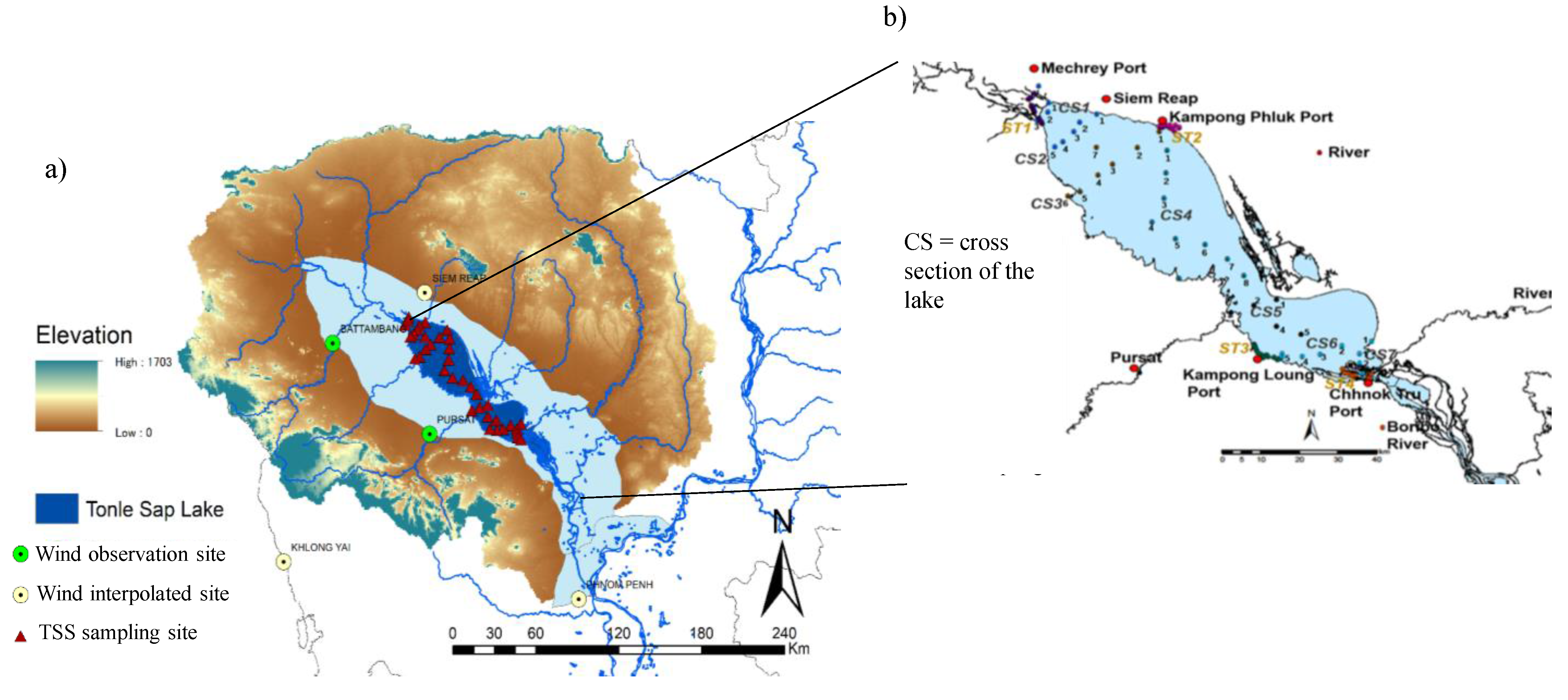
2.1. Study Area
2.2. Data Preparation
2.3. TSS and Other Environmental Variables
2.4. Empirical Relationships
2.5. Mechanism Elucidation of Wind-Induced Sediment Re-Suspension
3. Results and Discussion
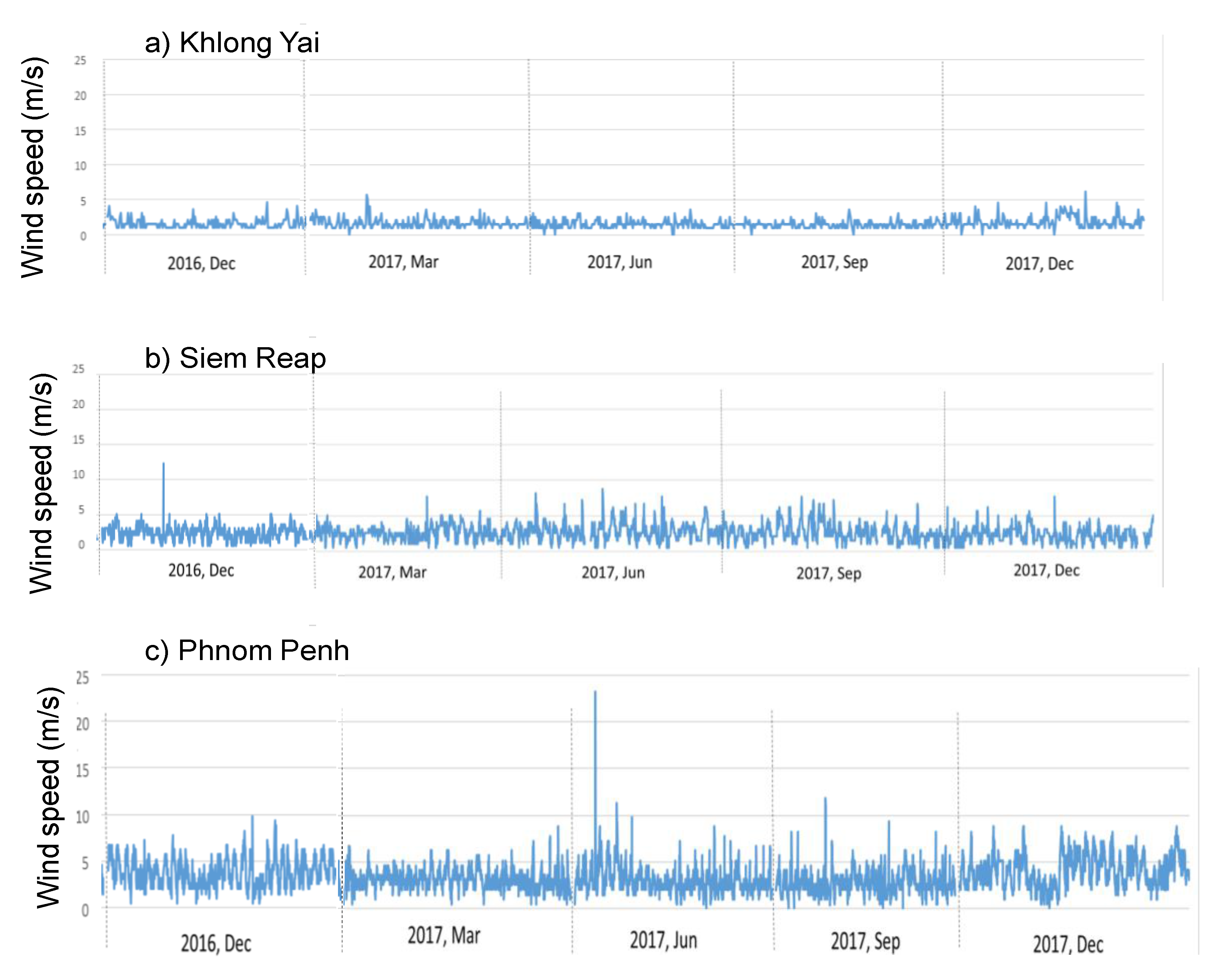
3.1. Characterization of Wind Data
3.2. Interpolation of Wind Data
3.3. Empirical Relation
3.4. Mechanism of Sediment Re-Suspension
3.5. Time to Reach Equilibrium TSS
4. Conclusions
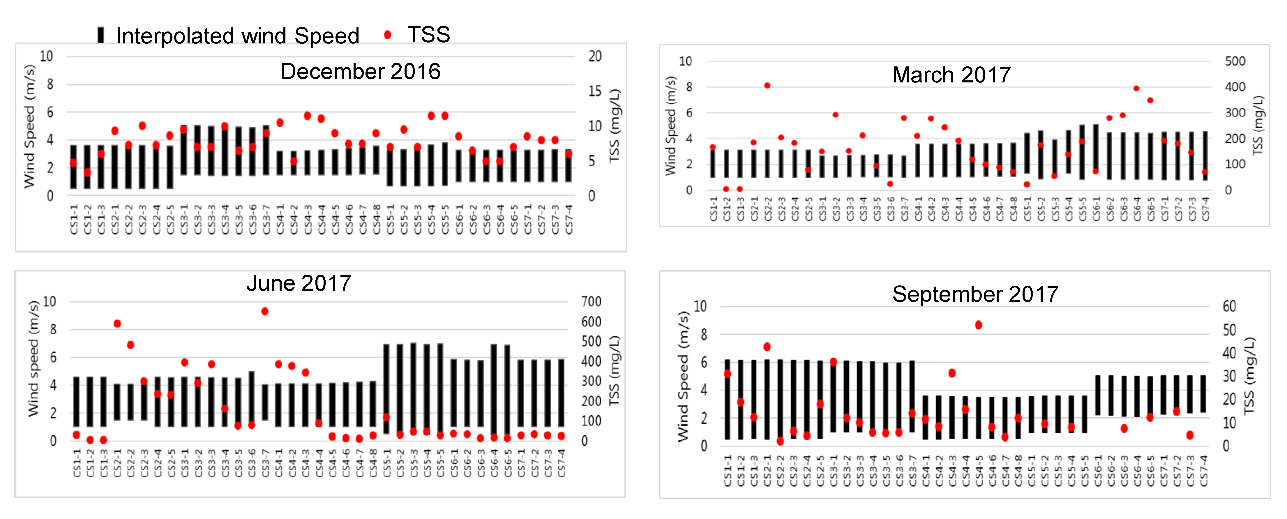
- In March, the wind direction is mainly southward and changes toward the southeast or southwest depending on the locations. In general, the wind speed in December and March was less than 5 m/s, but in June and September, the wind speed was as much 7 m/s.
- On the basis of the weighted Pearson correlation coefficient (r) and RMSE, wind interpolation using the IDW method was found to be comparatively better than the vectorized average and inverse of the ratio of distance.
- The TSS concentration, in general, during the wet season in December and September was less than 50 mg/L, but during the dry season in March and June, it was greater than 50 mg/L and peaked up to 400 mg/L in March and greater than 600 mg/L in June. The sediment characteristics with respect to sand, silt, and clay did not differ much across various CS in TSL.
- Settling velocity (m/day) across 37 sites across TSL varied from 0.28 to 11.70, with an average of 3.25 ± 2.75.
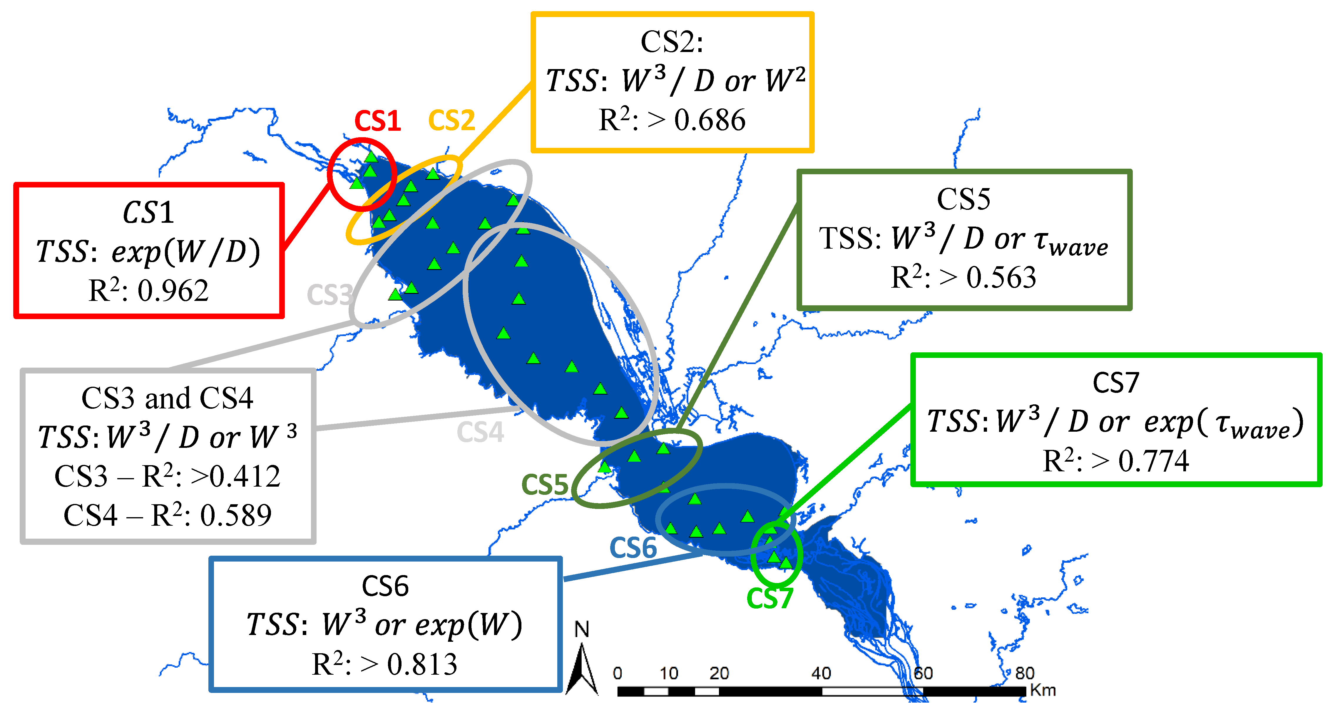
- TSS did not exhibit direct correlation with the settling velocity and sediment characteristics (LOI and particle diameter). The empirical equation to correlate TSS with wind speed (W), water depth (D), and shear stress (τ_wave), especially during dry season for different CS across TSL is, CS1= exp(W/D); CS2= W2 or W3/D; CS3, and CS4 = W3 or W3/D; CS5 = W3/D or τ_wave; CS6 = W3 or exp(W); and CS7 = W3/D or exp(τ_wave) (for detailed equation, please refer to Table 4).
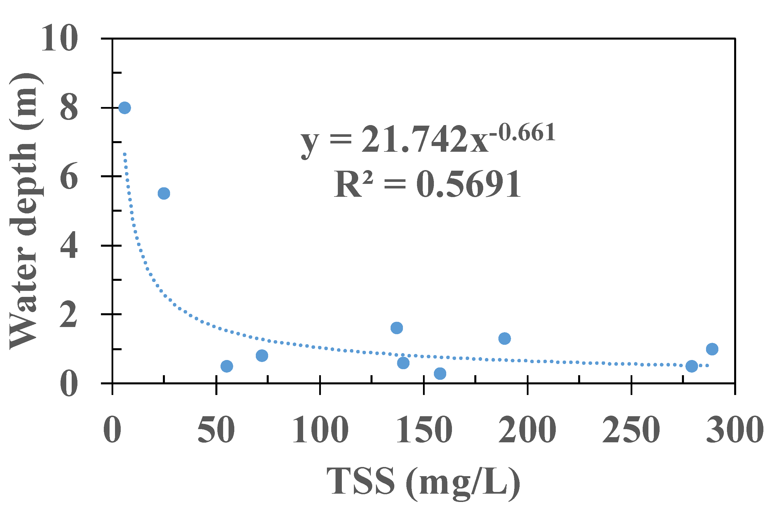
- The shear stress due to waves was smaller at the center of the lake and increased toward the shoreline, which is one of the reasons why TSL exhibits higher TSS at the shoreline than at the center of the lake. The total shear stress was greater than the critical shear stress, especially during the dry season in March, when TSS is higher and water depth is lower, compared to the wet season, when TSS is low and water depth is higher.
- The higher wind-induced critical shear stress than the total shear stress at most of the CS in TSL indicated sedimentation occurs predominantly during the transition phase of the reversal flow between TSL and MR during December and June, and erosion (siltation) is dominant during March. Additionally, most of the siltation in March was dominant in the southern part of the lake, at CS5, 6, and 7.
- The times to reach equilibrium TSS in March, June, and December were 9, 20, and 32 days, respectively. In general, the higher the depth is, the longer the time to reach equilibrium TSS.
Supplementary Materials
Author Contributions
Funding
Data Availability Statement
Acknowledgments
Conflicts of Interest
References
- Hawley, N.; Lesht, B. Sediment resuspension in Lake St. Clair. Limnol. Oceanogr. 1992, 37, 1720–1737. [Google Scholar] [CrossRef]
- Vlag, D.P. A model for predicting waves and suspended silt concentration in a shallow lake. Hydrobiologia 1992, 235, 119–131. [Google Scholar] [CrossRef]
- Barica, J. Extreme fluctuations in water quality of eutrophic fish kill lakes: Effect of sediment mixing. Water Res. 1974, 8, 881–888. [Google Scholar] [CrossRef]
- Hamilton, D.P.; Mitchell, S.F. An empirical model for sediment resuspension in shallow lakes. Hydrobiologia 1996, 317, 209–220. [Google Scholar] [CrossRef]
- Scheffer, M. Ecology of Shallow Lakes; Springer: Berlin, Germany, 2004; Volume 22. [Google Scholar]
- Reddy, K.R.; Fisher, M.M.; Ivanoff, D. Resuspension and diffusive flux of nitrogen and phosphorus in a hyper-eutrophic lake. J. Environ. Qual. 1996, 25, 363–371. [Google Scholar] [CrossRef]
- Søndergaard, M.; Kristensen, P.; Jeppesen, E. Phosphorus release from resuspended sediment in the shallow and wind-exposed Lake Arresø, Denmark. Hydrobiologia 1992, 228, 91–99. [Google Scholar] [CrossRef]
- Ogilvie, B.G.; Mitchell, S.F. Does sediment resuspension have persistent effects on phytoplankton? Experimental studies in three shallow lakes. Freshw. Biol. 1998, 40, 51–63. [Google Scholar] [CrossRef]
- Jalil, A.; Li, Y.; Zhang, K.; Gao, X.; Wang, W.; Khan, H.O.S.; Pan, B.; Ali, S.; Acharya, K. Wind-induced hydrodynamic changes impact on sediment resuspension for large, shallow Lake Taihu, China. Int. J. Sediment Res. 2019, 34, 205–215. [Google Scholar] [CrossRef]
- Chao, X.; Jia, Y.; Shields, F.D., Jr.; Wang, S.S.; Cooper, C.M. Three-dimensional numerical modeling of cohesive sediment transport and wind wave impact in a shallow oxbow lake. Adv. Water Resour. 2008, 31, 1004–1014. [Google Scholar] [CrossRef]
- Luettich, R.A., Jr.; Harleman, D.R.; Somlyody, L. Dynamic behavior of suspended sediment concentrations in a shallow lake perturbed by episodic wind events. Limnol. Oceanogr. 1990, 35, 1050–1067. [Google Scholar] [CrossRef]
- Horppila, J.; Nurminen, L. Effects of submerged macrophytes on sediment resuspension and internal phosphorus loading in Lake Hiidenvesi (Southern Finland). Water Res. 2003, 37, 4468–4474. [Google Scholar] [CrossRef]
- Matisoff, G.; Watson, S.B.; Guo, J.; Duewiger, A.; Steely, R. Sediment and nutrient distribution and resuspension in Lake Winnipeg. Sci. Total Environ. 2017, 575, 173–186. [Google Scholar] [CrossRef]
- Qin, B.; Zhu, G.; Zhang, L.; Luo, L.; Gao, G.; Gu, B. Estimation of internal nutrient release in large shallow Lake Taihu, China. Sci. China Ser. D 2006, 49, 38–50. [Google Scholar] [CrossRef]
- Bailey, M.C.; Hamilton, D.P. Wind induced sediment resuspension: A lake-wide model. Ecol. Model. 1997, 99, 217–228. [Google Scholar] [CrossRef]
- Morales-Marin, L.A.; French, J.R.; Burningham, H.; Battarbee, R.W. Three-dimensional hydrodynamic and sediment transport modeling to test the sediment focusing hypothesis in upland lakes. Limnol. Oceanogr. 2018, 63, S156–S176. [Google Scholar] [CrossRef] [Green Version]
- Bengtsson, L.; Hellström, T. Wild-induced resuspension in a small shallow lake. Hydrobiologia 1992, 241, 163–172. [Google Scholar] [CrossRef]
- Wu, T.; Timo, H.; Qin, B.; Zhu, G.; Janne, R.; Yan, W. In-situ erosion of cohesive sediment in a large shallow lake experiencing long-term decline in wind speed. J. Hydrol. 2016, 539, 254–264. [Google Scholar] [CrossRef]
- Carper, G.L.; Bachmann, R.W. Wind resuspension of sediments in a prairie lake. Can. J. Fish. Aquat. Sci. 1984, 41, 1763–1767. [Google Scholar] [CrossRef]
- Brocchini, M.; Dodd, N. Nonlinear shallow water equation modeling for coastal engineering. J. Waterw. Port Coast. Ocean Eng. 2008, 134, 104–120. [Google Scholar] [CrossRef]
- Rohweder, J.J.; Rogala, J.T.; Johnson, B.L.; Anderson, D.; Clark, S.; Chamberlin, F.; Runyon, K. Application of wind fetch and wave models for habitat rehabilitation and enhancement projects. Geol. Surv. 2008, 1200, 43. [Google Scholar]
- Håkanson, L.; Bryhn, A.C. A dynamic mass-balance model for phosphorus in lakes with a focus on criteria for applicability and boundary conditions. Water Air Soil Pollut. 2007, 187, 119–147. [Google Scholar] [CrossRef] [Green Version]
- Siev, S.; Yang, H.; Sok, T.; Uk, S.; Song, L.; Kodikara, D.; Oeurng, C.; Hul, S.; Yoshimura, C. Sediment dynamics in a large shallow lake characterized by seasonal flood pulse in Southeast Asia. Sci. Total Environ. 2018, 631, 597–607. [Google Scholar] [CrossRef]
- Reeks, M.W.; Reed, J.R.; Hall, D.R. On the resuspension of small particles by a turbulent flow. J. Phys. D Appl. Phys. 1988, 21, 574–589. [Google Scholar] [CrossRef]
- Churchill, J.H.; Williams, A.J.; Ralph, E.A. Bottom stress generation and sediment transport over the shelf and slope off of Lake Superior’s Keweenaw peninsula. J. Geophys. Res. Ocean. 2004, 109, 10.1029/2003JC001997. [Google Scholar] [CrossRef]
- Chung, E.G.; Bombardelli, F.A.; Schladow, S.G. Sediment resuspension in a shallow lake. Water Resour. Res. 2009, 45. [Google Scholar] [CrossRef]
- Hawley, N.; Lesht, B.M.; Schwab, D.J. A comparison of observed and modeled surface waves in southern Lake Michigan and the implications for models of sediment resuspension. J. Geophys. Res. Space Phys. 2004, 109. [Google Scholar] [CrossRef] [Green Version]
- Zhang, S.; Nielsen, P.; Perrochet, P.; Jia, Y. Multiscale superposition and decomposition of field-measured suspended sediment concentrations: Implications for extending 1DV models to coastal oceans with advected fine sediments. J. Geophys. Res. Ocean. 2021, 126, e2020JC016474. [Google Scholar] [CrossRef]
- Zhang, S.; Wu, J.; Jia, Y.; Wang, Y.-G.; Zhang, Y.; Duan, Q. A temporal LASSO regression model for the emergency forecasting of the suspended sediment concentrations in coastal oceans: Accuracy and interpretability. Eng. Appl. Artif. Intell. 2021, 100, 104206. [Google Scholar] [CrossRef]
- Ji, Z.-G.; Jin, K.-R. Impacts of wind waves on sediment transport in a large, shallow lake. Lakes Reserv. Res. Manag. 2014, 19, 118–129. [Google Scholar] [CrossRef]
- Reardon, K.E.; Bombardelli, F.A.; Moreno-Casas, P.A.; Rueda, F.J.; Schladow, S.G. Wind-driven nearshore sediment resuspension in a deep lake during winter. Water Resour. Res. 2014, 50, 8826–8844. [Google Scholar] [CrossRef]
- Miao, Q.; Yang, D.; Yang, H.; Li, Z. Establishing a rainfall threshold for flash flood warnings in China’s mountainous areas based on a distributed hydrological model. J. Hydrol. 2016, 541, 371–386. [Google Scholar] [CrossRef]
- Sheng, Y.P.; Lick, W. The transport and resuspension of sediments in a shallow lake. J. Geophys. Res. Space Phys. 1979, 84, 1809–1826. [Google Scholar] [CrossRef]
- Kummu, M.; Penny, D.; Sarkkula, J.; Koponen, J. Sediment: Curse or blessing for Tonle Sap Lake? AMBIO J. Hum. Environ. 2008, 37, 158–163. [Google Scholar] [CrossRef]
- Koehnken, L. IKMP Discharge and Sediment Monitoring Program Review, Recommendations and Data Analysis—Part 2: Data Analysis and Preliminary Results; Mekong River Commission (MRC): Phnom Penh, Cambodia, 2012. [Google Scholar]
- Shivakoti, B.R.; Ngoc-Bao, P. Environmental Changes in Tonle Sap Lake and Its Floodplain: Status and Policy Recommendations; Institute for Global Environmental Strategies (IGES): Kanagawa, Japan; Tokyo Institute of Technology (Tokyo Tech): Tokyo, Japan; Institute of Technology of Cambodia (ITC): Phnom Penh, Cambodia, 2020. [Google Scholar]
- Tsukawaki, S. Lithological features of cored sediments from the northern part of Lake Tonle Sap, Cambodia. In Proceedings of the International Conference on Stratigraphy and Tectonic Evolution of Southeast Asia and the South Pacific, Bangkok, Thailand, 19–24 August 1997; pp. 232–239. [Google Scholar]
- Ali, S.M.; Mahdi, A.S.; Shaban, A.H. Wind speed estimation for Iraq using several spatial interpolation methods. Environ. Prot. 2012, 1, 2. [Google Scholar]
- Bretschneider, F.; De Weille, J.R. Introduction to Electrophysiological Methods and Instrumentation; Elsevier: Amsterdam, The Netherlands, 2006. [Google Scholar]
- James, W.F.; Barko, J.W.; Butler, M.G. Shear stress and sediment resuspension in relation to submersed macrophyte biomass. Hydrobiologia 2004, 515, 181–191. [Google Scholar] [CrossRef]
- Parker, G.; Toro-Escobar, C.M.; Ramey, M.; Beck, S. Effect of floodwater extraction on mountain stream morphology. J. Hydraul. Eng. 2003, 129, 885–895. [Google Scholar] [CrossRef]
- Khanal, R.; Uk, S.; Kodikara, D.; Siev, S.; Yoshimura, C. Impact of water level fluctuation on sediment and phosphorous dynamics in Tonle Sap Lake, Cambodia. Water Air Soil Pollut. 2021, 232, 1–15. [Google Scholar] [CrossRef]
- Gloor, M.; Wüest, A.; Münnich, M. Benthic boundary mixing and resuspension induced by internal seiches. Hydrobiologia 1994, 284, 59–68. [Google Scholar] [CrossRef]


| IDW | Pursat | Battam Bang | Average | |||||||
|---|---|---|---|---|---|---|---|---|---|---|
| Year | 2008 | 2009 | 2010 | 2010 | ||||||
| Evaluation Value | r | RMSE | r | RMSE | r | RMSE | r | RMSE | r | RMSE |
| (1) Speed | ||||||||||
| IDW | 0.75 | 0.68 | 0.57 | 0.70 | 0.31 | 1.19 | 0.32 | 0.70 | 0.49 | 0.81 |
| Vectorized average | 0.78 | 1.11 | 0.36 | 1.26 | 0.20 | 1.96 | −0.14 | 0.84 | 0.30 | 1.29 |
| Inverse of ratio | 0.55 | 0.91 | 0.17 | 0.98 | 0.56 | 1.65 | −0.05 | 0.96 | 0.31 | 1.13 |
| (2) Direction | ||||||||||
| IDW | −0.35 | 122 | −0.11 | 162 | 0.60 | 255 | −0.19 | 163 | −0.01 | 176 |
| Vectorized average | 0.31 | 56 | 0.34 | 176 | −0.58 | 192 | −0.12 | 83 | −0.01 | 127 |
| Inverse of ratio | 0.24 | 142 | 0.27 | 145 | 0.12 | 284 | −0.43 | 177 | 0.05 | 187 |
| (3) Direction + Speed (Inner product) | ||||||||||
| r | ||||||||||
| IDW | −0.02 | −0.28 | 0.14 | 0.07 | −0.02 | −0.02 | ||||
| Vectorized average | 0.06 | 0.05 | 0.00 | −0.24 | −0.03 | 0.06 | ||||
| Inverse of ratio | −0.45 | 0.07 | 0.66 | −0.40 | −0.03 | −0.45 | ||||
| (4) Direction + Speed (Polar coordinates) | ||||||||||
| r | x | y | x | y | x | y | x | y | x | y |
| IDW | 0.32 | −0.63 | 0.25 | 0.01 | −0.55 | 0.24 | 0.54 | −0.62 | 0.14 | −0.25 |
| Vectorized average | 0.64 | 0.61 | 0.55 | 0.40 | 0.04 | −0.30 | 0.23 | 0.22 | 0.36 | 0.23 |
| Inverse of ratio | 0.89 | 0.33 | −0.42 | −0.90 | 0.49 | −0.24 | 0.48 | 0.37 | 0.36 | −0.11 |
| RMSE | x | y | x | y | x | y | x | y | x | y |
| IDW | 1.21 | 3.38 | 2.37 | 3.30 | 0.57 | 3.48 | 1.39 | 4.02 | 1.39 | 3.55 |
| Vectorized average | 1.19 | 1.30 | 2.92 | 1.92 | 0.55 | 1.05 | 1.53 | 1.56 | 1.55 | 1.46 |
| Inverse of ratio | 1.32 | 3.11 | 1.37 | 2.85 | 1.32 | 3.13 | 0.26 | 3.80 | 1.07 | 3.22 |
| Month | Wind | Total Suspended Solid (TSS) | |
|---|---|---|---|
| Wind Direction | Wind Speed | ||
|
| ||
| December | Direction changes to N at once 1: Trends change slightly between 2016 and 2017, but mainly is westward 2,3: Direction changes to N at once | 1: Higher in 2017 than in 2016, and similar in range as in Mar 2: Max: 12.3 m/s, turbulence calms down compared to Sep 3: Average increases compared to Sep |
|
| March | Trends do not change regardless of year 1: Main direction: West or East wind, No NE or SW direction 2: Frequent southern wind, relatively unstable 3: Only SE in 2016 and 2017 | 1: Relatively lower wind speed (Ave: 3–4 m/s, max: 3.6–5.7 m/s) 2: Occasional stronger wind (7.2–8.2 m/s) 3: Max: 6.2–8.8 m/s |
|
| June | Trends do not change regardless of year 1: NS from EW in Mar 2: SW stable 3: SW to SE in Mar | 1: Average does not change in Mar, max changes (3.6 m/s in Mar → 15.4 m/s in Jun) 2: Increases by 5 m/s from 7.2–8.2 → 8.8–13.3 m/s 3: Speed does not change, with occasional max, 6.2–8.8 → 12.9–23.2 m/s |
|
| September | Trends do not change regardless of year 1: Frequent westward, 2016 and 2017 show same trends. 2: Overall westward, NW ratio increases in 2017 3: S and N from SW 4: Westward wind trend remainsDirection varies by year | 1: No turbulence and a stable wind of 2–3 m/s 2: 15–20 m/s in 2016, no turbulence and a stable wind around 7 m/s 3: Speed is the same or slightly higher than that in Jun at around 10 m/s |
|
| Area | Point | Settling Velocity (m/day) | Mass Ratio of Sediment (%, Sand, Silt, Clay) | |
|---|---|---|---|---|
| CS1 | CS1-1 | 6.50 | 4.16 |  |
| CS1-2 | 6.48 | 4.14 |  | |
| CS1-3 | 5.08 | 2.55 |  | |
| CS2 | CS2-1 | 6.78 | 4.53 |  |
| CS2-2 | 4.86 | 2.33 |  | |
| CS2-3 | 5.50 | 2.98 |  | |
| CS2-4 | 5.61 | 3.11 |  | |
| CS2-5 | 7.84 | 6.05 |  | |
| CS3 | CS3-1 | 6.87 | 4.65 |  |
| CS3-2 | 5.48 | 2.96 |  | |
| CS3-3 | 5.65 | 3.15 |  | |
| CS3-4 | 3.42 | 1.16 |  | |
| CS3-5 | 10.9 | 11.7 |  | |
| CS3-6 | 9.36 | 8.65 |  | |
| CS3-7 | 4.46 | 1.96 |  | |
| CS4 | CS4-1 | 2.49 | 0.61 |  |
| CS4-2 | 6.28 | 3.89 |  | |
| CS4-3 | 2.28 | 0.51 |  | |
| CS4-4 | 2.62 | 0.68 |  | |
| CS4-5 | 3.00 | 0.89 |  | |
| CS4-6 | 6.48 | 4.14 |  | |
| CS4-7 | 5.83 | 3.35 |  | |
| CS4-8 | 2.71 | 0.72 |  | |
| CS5 | CS5-1 | 5.85 | 3.37 |  |
| CS5-2 | 4.80 | 2.27 |  | |
| CS5-3 | 8.01 | 6.33 |  | |
| CS5-4 | 1.68 | 0.28 |  | |
| CS5-5 | 2.02 | 0.40 |  | |
| CS6 | CS6-1 | 7.38 | 5.37 |  |
| CS6-2 | 4.19 | 1.73 |  | |
| CS6-3 | 2.15 | 0.46 |  | |
| CS6-4 | 3.94 | 1.53 |  | |
| CS6-5 | 3.10 | 0.95 |  | |
| CS7 | CS7-1 | 7.83 | 6.05 |  |
| CS7-2 | 3.49 | 1.20 |  | |
| CS7-3 | 10.3 | 10.4 |  | |
| CS7-4 | 3.31 | 1.08 |  |
| Regression Relation | R2 | RMSE | |
|---|---|---|---|
| Whole lake (dry + wet season) | 0.06 | 111 | |
| Wet season | 0.03 | 2.0 | |
| 0.02 | 2.0 | ||
| Dry season | 0.06 | 141 | |
| Dry season | |||
| Cross section 1 | 0.96 | 53 | |
| Cross section 2 | 0.71 | 259 | |
| 0.69 | 256 | ||
| Cross section 3 | 0.42 | 198 | |
| 0.41 | 182 | ||
| Cross section 4 | 0.59 | 159 | |
| 0.59 | 156 | ||
| Cross section 5 | 0.56 | 79 | |
| 0.58 | 73 | ||
| Cross section 6 | 0.82 | 175 | |
| 0.81 | 153 | ||
| Cross section 7 | 0.88 | 82 | |
| 0.77 | 51 |
| Date | Point | TSS (mg/L) | Water Depth (m) | Total Shear Stress (Pa) | Critical Shear Stress (Pa) |
|---|---|---|---|---|---|
| 21 December 2016 | CS7-4 | 6 | 8.0 | 2.93 | 1.63 |
| 30 March 2017 | CS5-2 | 158 | 0.3 | 5.85 | 2.36 |
| 15 March 2017 | CS5-4 | 55 | 0.5 | 3.30 | 3.94 |
| 16 March 2017 | CS5-4 | 137 | 1.6 | 2.53 | 0.83 |
| 26 March 2017 | CS5-5 | 140 | 0.6 | 2.26 | 0.83 |
| 15 March 2017 | CS6-2 | 189 | 1.3 | 3.06 | 2.06 |
| 15 March 2017 | CS6-5 | 72 | 0.8 | 1.76 | 1.52 |
| 15 March 2017 | CS7-1 | 279 | 0.5 | 5.81 | 3.85 |
| 15 March 2017 | CS7-4 | 289 | 1.0 | 3.25 | 1.63 |
| 2 July 2017 | CS7-4 | 25 | 5.5 | 2.66 | 1.63 |
| March (2017) | June (2017) | December (2016) | ||
|---|---|---|---|---|
| Observed TSS (mg/L) | 433 | 684 | 15.5 | |
| 4.5 | 12 | 4.3 | ||
| Ave | 176.8 | 157.4 | 4.8 | |
| Average wind speed (m/s) (W) | 2.3 | 2.5 | 2.4 | |
| Average water depth (m) (D) | 1.2 | 2.8 | 4.7 | |
| Average settling velocity (m/day) (β) | 3.2 | 3.3 | 3.3 | |
| Time for equilibrium TSS (day) | 9 | 20 | 32 | |
Publisher’s Note: MDPI stays neutral with regard to jurisdictional claims in published maps and institutional affiliations. |
© 2021 by the authors. Licensee MDPI, Basel, Switzerland. This article is an open access article distributed under the terms and conditions of the Creative Commons Attribution (CC BY) license (https://creativecommons.org/licenses/by/4.0/).
Share and Cite
Sato, M.; Khanal, R.; Uk, S.; Siev, S.; Sok, T.; Yoshimura, C. Impact of Wind on the Spatio-Temporal Variation in Concentration of Suspended Solids in Tonle Sap Lake, Cambodia. Earth 2021, 2, 424-439. https://doi.org/10.3390/earth2030025
Sato M, Khanal R, Uk S, Siev S, Sok T, Yoshimura C. Impact of Wind on the Spatio-Temporal Variation in Concentration of Suspended Solids in Tonle Sap Lake, Cambodia. Earth. 2021; 2(3):424-439. https://doi.org/10.3390/earth2030025
Chicago/Turabian StyleSato, Michitaka, Rajendra Khanal, Sovannara Uk, Sokly Siev, Ty Sok, and Chihiro Yoshimura. 2021. "Impact of Wind on the Spatio-Temporal Variation in Concentration of Suspended Solids in Tonle Sap Lake, Cambodia" Earth 2, no. 3: 424-439. https://doi.org/10.3390/earth2030025
APA StyleSato, M., Khanal, R., Uk, S., Siev, S., Sok, T., & Yoshimura, C. (2021). Impact of Wind on the Spatio-Temporal Variation in Concentration of Suspended Solids in Tonle Sap Lake, Cambodia. Earth, 2(3), 424-439. https://doi.org/10.3390/earth2030025