Mapping Susceptibility to Debris Flows Triggered by Tropical Storms: A Case Study of the San Vicente Volcano Area (El Salvador, CA)

Abstract

In this study, an inventory of storm-triggered debris flows performed in the area of the San Vicente volcano (El Salvador, CA) was used to calibrate predictive models and prepare a landslide susceptibility map. The storm event struck the area in November 2009 as the result of the simultaneous action of low-pressure system 96E and Hurricane Ida. Multivariate Adaptive Regression Splines (MARS) was employed to model the relationships between a set of environmental variables and the locations of the debris flows. Validation of the models was performed by splitting 100 random samples of event and non-event 10 m pixels into training and test subsets. The validation results revealed an excellent (area under the receiver operating characteristic (ROC) curve (AUC) = 0.80) and stable (AUC std. dev. = 0.01) ability of MARS to predict the locations of the debris flows which occurred in the study area. However, when using the Youden’s index as probability threshold to discriminate between pixels predicted as positives and negatives, MARS exhibits a moderate ability to identify stable cells (specificity = 0.66). The final debris flow susceptibility map, which was prepared by averaging for each pixel the score of the 100 MARS repetitions, shows where future debris flows are more likely to occur, and thus may help in mitigating the risk associated with these landslides.

1. Introduction

Landslides are among the main causes of natural hazards in El Salvador [1]. In these areas, landslides are caused by tropical rains or occur as a secondary event of earthquakes. Regarding the first trigger, the intense rainfall events that frequently affect the country are responsible for the activation of gravitational phenomena consisting of shallow and fast-moving flow landslides that may cause severe economic damage and even victims [2]. The occurrence of these landslides is related to the outcropping of unconsolidated material on steep slopes, which can be rapidly moved by gravity and travel hundreds of meters to several kilometers from its origin [3]. Dramatic examples of their destructive potential are given by the disasters which occurred in Vargas (Venezuela), causing around 15,000 victims in December 1999 [4,5], or in the mountainous regions of Rio de Janeiro (Brazil), in January 2001, where numerous debris avalanches and debris flows triggered by an extreme rain event lasting 2 days caused around 1500 victims [6,7].

Landslide risk can be mitigated by predicting the areas in which slope failures are most likely to occur in the future. The likelihood of a gravitational phenomenon triggering in a specific location is known as landslide susceptibility. A landslide susceptibility map represents, for each spatial unit of a given area, the relative probability of landslide occurrence [8,9]. Developing landslide susceptibility maps provides a valid and useful tool to the authorities dealing with territory management and civil protection, as they indicate where new slope failures are more likely to occur.

Several methodologies could be used to generate landslide susceptibility maps. At watershed or regional scale, the probability of landslide occurrence is mostly evaluated by adopting a stochastic approach [10,11,12,13,14,15,16,17,18,19]. This is based on the principle that “the past is the key to the future”, thus the triggering of future landslides is more probable under the same environmental conditions that produced slope failures in the past. A statistical approach relies upon inventories of landslides and maps revealing the spatial variability of a set of environmental attributes, expressing the time-unchanging preparatory conditions allowing the reproduction of the morphodynamic response to a given future triggering event. The dependent variable reflects the presence or absence of landslides in a given location or mapping unit. The independent variables (or covariates) act as proxies to the factors mainly controlling landslide occurrence in the study area and are expected to play the role of predictors of the spatial distribution of the landslides included in the inventories [20]. Once a set of predictors is defined, a value for dependent and independent variables is assigned to each of the mapping units [21]. Unlike geomorphological or heuristic methods, which strongly depend on the skill and experience of the operator, the stochastic approach is characterized by a high objectivity since it uses statistical tools to determine the influence of the instability factors and, consequently, the functional relationship between the latter and the distribution of gravitational phenomena in a given area [22]. The statistical approach aims to achieve the best possible compromise between costs (money and time) and reliability of the landslide susceptibility models. The quality of the input data strongly controls the accuracy of the landslide predictive models and the relative susceptibility maps. At the same time, deterministic approaches are critically dependent on very strong hypothesis about mechanical and hydrological properties of rocks, layering and geometrical setting of shallow to deep volumes, failure mechanisms and surface type, triggering rainfall function [23].

In this study, remote analysis allowed us to prepare to prepare an inventory of landslides that occurred in San Vicente (El Salvador), following a combination of events that hit El Salvador in November 2009, when most of the country was affected by the passage of Hurricane Ida and low-pressure system 96E. Most of the landslides which occurr in San Vicente can be classified as debris flows. According to the Varnes classification of landslides [24], debris flows are characterized by a mixture of non-cohesive material (<80% sand and finer), air and water that rapidly move downwards along impluvium lines, usually gullies and first- or second-order channels. From a physical-mechanical aspect, debris flows are viscous fluids that are in an intermediate position between rock avalanches and sediment-laden water floods. Debris flows can be initiated by debris slides or avalanches or rock falls occurring on open and steep slopes. Once the moving material reaches steep impluvium lines, these phenomena turns into debris flows [25]. These consist of surges of rock masses, air, and water that move downstream along the channels, entraining saturated soil and surface water [7]. In this phase, the speed of such gravitational phenomena is considerable (up to 20 m/s), and different debris flows can also flow into the same channel, thus increasing their erosive and destructive power. The deposition fan is often located at the base of the slope, but can also reach several kilometers from it. For this reason, this type of landslide is extremely dangerous in the San Vicente area, where the base of the volcano slopes is densely populated and crossed by major transportation routes.

The aim of this work is to predict the spatial distribution of the landslides occurring in the San Vicente area by using a statistical modelling technique known as Multivariate Adaptive Regression Splines (MARS) [26]. The MARS method has been successfully applied recently in some geomorphological studies [27,28,29,30], but there are relatively few tests in the literature in the field of landslide susceptibility zoning [9,27,28,29,31,32,33,34,35,36]. In fact, the statistical techniques most frequently used to map landslide susceptibility in the recent past have been conditional analysis, discriminant analysis, logistic regression, artificial neural networks, and classification and regression trees [18,20,21,37,38,39,40,41]. The performance of the model is evaluated by using confusion matrices and by preparing receiver operating characteristic (ROC) curves and analyzing the values of the area under the ROC curve (AUC).

2. Geographical Description and Mapping

2.1. Study Area

The study area, which extends for 287 km², is located along the slopes of the San Vicente Volcano, El Salvador, CA (Figure 1).

The San Vicente volcano, also known as Chichontepec (in the indigenous language nawat pipil language it means “the mountain of the two breasts” for its double summit) is one of the 22 volcanoes of the volcanic arc of El Salvador and is situated next to the town of San Vicente (hence the name), located about 50 km east of the capital city San Salvador. This composite stratovolcano is the second highest volcano (2182 m asl) and one of the most important volcanos in the country (with San Salvador, San Miguel, Ilopango, Santa Ana, lzalco, and Conchaguita).

Although San Vicente has not erupted in the past 1700 years, powerful hot springs and geothermal developments located on the north side of the volcano suggest that past eruptions are youthful enough and that the volcanic system maintains residual heat from magmatic sources. Thus, the volcano should be considered active and likely to erupt again [42].

Predicting the style of future eruptions is difficult due to the poorly-known eruptive history, however, on the basis of past eruptive activity, future eruptions might involve emplacement of lava flows and growth and collapse of small-volume lava domes. In addition, the collapse of lava domes might generate pyroclastic flows and surges that might travel several kilometers over the volcano’s base.

However, possible future eruptions do not represent the main problem posed by the volcano, as the main current risk in the area is given by the manifestation of massive debris flows.

Due to a tropical-humid climate regime, with average annual rainfall of about 1500 mm and average annual temperatures between 21 °C and 32 °C, the slopes of San Vicente volcano experience strong physical-chemical degradation with consequent lowering of the level of cohesion of the rocks, also favored by the pyroclastic and ashy nature of the outcropping materials. This climatic and geological setting favors the occurrence of numerous gravitational phenomena, such as debris flows, involving weathered pyroclastic materials which cover steep slopes. This type of landslide, which can destroy or damage everything in its path through burial or impact, has occurred many times in Central America, causing enormous economic damage and, above all, deaths. For example, in 1998, at Casita volcano in Nicaragua, extremely heavy rainfall from Hurricane Mitch triggered rapidly moving debris flows that destroyed two villages and killed more than 2000 people. Regarding our study area, an impressive debris flow in 1934 on the north side of San Vicente destroyed the village of Tepetitan [42].

2.2. Landslide Inventory

On the 7 and 8 November 2009, most of El Salvador was struck by the simultaneous action of the Hurricane Ida and the low-pressure system 96E. Hurricane Ida has been evolving since 4 November 2009 as a tropical depression in the southern-western sector of the Caribbean Sea and increased its strength until it evolved to tropical storm grade on 7 November while crossing Nicaragua’s coast. It arrived at the stage of second level hurricane on the 8, then subsequently shifted northward to the Gulf of Mexico and the Caribbean Sea, returning to the tropical storm grade and then depression on the 9, until its total disappearance on 12 November. At the same time, the low-pressure system 96E from the eastern Pacific Ocean arrived in El Salvador territory [43]. This event caused heavy rainfall between 7 and 8. The combined action of these two events resulted in about 350 mm in 24 h in an area of about 400 km² located between Ilopango Lake and San Vicente Volcano.

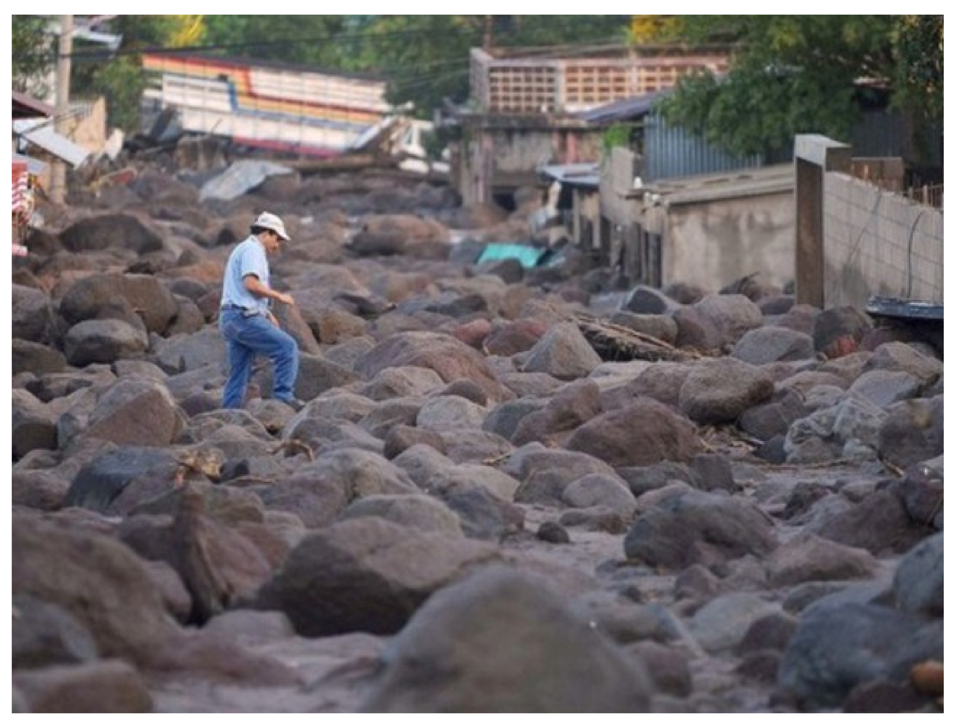
As a consequence, floods and thousands of landslides occurred in this area, causing about 200 victims, huge damage to infrastructures and buildings, with an economic loss estimated to be approximately a quarter of a billion dollars [44]. These landslides, mostly debris flows, seriously affected the villages of Verapaz and Guadalupe (Figure 2 and Figure 3), located in the north-western sector of the study area. By comparing the two images of Figure 2, it is possible to identify numerous debris flows, which mainly occurred on the northern and north-western flanks of the volcano, hitting the towns of Guadalupe and Verapaz, located at 5 and 6 km NW from the volcano summit. The triggering of the slope instability at the initiation point was due to the increase in pore pressure and unit weight induced by the saturation of the top volcanic layer. The debris flows phenomena triggered a debris slide at the initiation points rapidly moving downward and taking the form of debris avalanches/debris flows entraining large part of the weathered pyroclastic top-layer. In light of their high energy, the flows which moved from the head sector of the northern volcanic slopes took the form of huge debris flows entraining also the alluvial block/gravel debris along the gullies and the streams which assumed the role of tracks.

Mapping of the landslides triggered by heavy rainfalls in a tropical area, where vegetation recovers rapidly, such as that of San Vicente, requires aerial/satellite images taken not long after the event. The landslides archive used in this study was prepared by remotely analyzing high-resolution imagery dated 21 November 2009, thus only 2 weeks after the combined action of Hurricane Ida and 96E low-pressure system, and freely available in Google Earth. Each debris flow was delimited into a polygon and a landslide identification point (LIP; [39]) which was automatically extracted at the highest point of the landslide crown line. Although no agreement exists on the best location of a point allowing to identify for a given landslide the conditions that triggered that specific slope failure, numerous recent studies have successfully adopted LIPs for landslide susceptibility zoning [40,45,46]. In case of debris flows, which are usually shallow, LIPs are expected to be even more suitable to identify pre-failure conditions [34,45].

2.3. Environmental Variables

Landslide susceptibility zoning requires the adoption of a mapping unit technique, which allows the study area to be divided into portions with certain properties, and to distinguish each unit from adjacent ones according to clear and definable boundaries [15]. The selection of a type of mapping unit depends on the available data and on the objective of the research. In this study, grid cells were used as mapping units. These divide the territory into regular squares of predefined size and are usually preferred when working with raster data. The size of the cells was set to 10 m, in light of the horizontal resolution of the available digital elevation model (DEM), which was derived by vectorizing 10 m contour interval topographic maps and employed to derive most of the predictor variables. This resolution of the input data has been demonstrated to produce landslide susceptibility models with good predictive performance [41]. For all of the selected independent variables, a value or a category was assigned to each cell. Regarding the dependent variable, which reflects the presence or absence of a LIP within a mapping unit, a binary value was given to each cell (0: absence; 1: presence) [39].

In this study, 10 environmental attributes were selected as predictor variables of the mapped landslide, on the basis of their presumed influence on the triggering mechanism and on the availability of data: GEO (lithology), USE (land use), LCL (landform classification), SLO (slope), ELE (elevation), PRC (profile curvature), PLC (plan curvature), TWI (topographic wetness index), NORTH (Northness), and EAST (Eastness). All the variables, with the exception of GEO and USE, were derived from the 10 m resolution raster DEM available for the area by using QGIS and SAGA GIS [47] software. GEO, USE, and LCL are categorical variables whereas all the others are continuous.

Geology (GEO)—The lithology layer was prepared on the basis a regional geological map at a scale of 1:100,000 [48], which was modified and improved by means of field checks. The study area is characterized by the presence of seven lithological units that can be distinguished on the basis of their different physic-chemical characteristics (Figure 4). In light of the expected physical behavior, to each of the different outcropping lithologies an expected geomechanical response was associated distinguishing soft (low cohesion and strength) from hard (high cohesion and shear strength) rock and soil terms.

In the area of the San Vicente volcano, the outcropping rocks are intermediate and basic effusive rocks with alternations of pyroclastites (geo.1). Moving eastward from the crater, large outcroppings of intermediate basic effusive rocks and subordinate pyroclastites (geo.3) can be observed, alternating with acid pyroclastic rocks, volcanic epiclastites and volcanic epiclastites and pyroclastites with locally effusive basic-intermediate rocks (geo.6 and geo.7) in the western sector of the area. In the northern sector, where the localities of San Vicente (north-eastern sector of the area), Guadalupe and Verapaz (north and north-western sector) are located, there is a strong presence of acidic pyroclastites and subordinate volcanic epiclastites and acid effusive rocks, or lithologies belonging to the Terra Blanca, a member of the San Salvador formation (geo.4). All these deposits are highly weathered and may favor the triggering of debris flows following intense rainfall events.

As shown in

Table 1. The seven lithological classes are shown with their corresponding descriptions and the percentage value of the presence of each class compared to the total area.

COD	TYPE	DESCRIPTION	% Presence of the Factor in the Area
geo.1	Soft rocks	intermediate basic effusive rocks and subordinate pyroclastites	23.00%
geo.2	Hard rocks	intermediate basic effusive rocks and subordinate pyroclastites	20.84%
geo.3	Medium rocks	acid effusive and acid intermediate rocks	0.80%
geo.4	Very soft soil	Tierra Blanca: acidic pyroclastites and subordinate volcanic epiclastites and acid effusive rocks	17.25%
geo.5	Soft soil	Quaternary sedimentary deposits	0.91%
geo.6	Hard soil	acid pyroclastic rocks, volcanic epiclastites	29.77%
geo.7	Medium soil	volcanic epiclastites and pyroclastites, locally effusive basic-intermediate rocks	7.42%

, the lithology class with the largest extent is that of hard soil, i.e., acid pyroclastic rocks and volcanic epiclastites; this class contains almost half of the identified landslides.

Land use (USE)—The land use raster map includes 11 classes and was created by rasterizing the Corine Land Cover shapefile, which was prepared by using satellite images dated 2002. Most of the territory investigated is characterized by crops of different nature, whereas only about 3% of the area is characterized by the presence of anthropogenic structures (

Table 2. Percentage frequency distribution of land use (left) and landform classifications (right).

COD	TYPE	% Presence of the Factor in the Area	COD	TYPE	% presence of the Factor in the Area
use.1	Urban areas	3.13%	lcl.0	Streams	4.86%
use.2	Woods	5.05%	lcl.1	Midslope drainages	7.88%
use.3	Annual crops	17.61%	lcl.2	Upland drainages	0.59%
use.4	Mixed crops	20.11%	lcl.3	Valleys	5.39%
use.5	Permanent crops	45.96%	lcl.4	Plains	18.21%
use.6	Wetlands	0.00%	lcl.5	Open slopes	42.47%
use.7	Mangroves	0.00%	lcl.6	Upper slopes	7.12%
use.8	Minings	0.00%	lcl.7	Local ridges	0.41%
use.9	Pastures	1.73%	lcl.8	Midslope ridges	8.98%
use.10	Rivers	0.24%	lcl.9	High ridges	4.08%
use.11	Shrub vegetations	6.18%

).

Landform classification (LCL)—This variable was extracted by using an automated procedure that recognizes landforms on a gridded elevation distribution. Table 2 reveals that open slopes (lcl.5) is the most frequent class.

Slope (SLO)—This variable represents the steepness of the ground measured as a percentage.

Elevation (ELE)—The altitude above sea level of each cell corresponds to the value of the DEM.

Profile curvature (PRC)—This variable reflects the geometry of the surface in the direction of the maximum incline of the slope. Positive cell values indicate an upward convexity of the surface while negative values indicate a downward concavity; a value of 0 indicates the absence of concavity/convexity and therefore a constant slope steepness.

Plan curvature (PLC)—This variable reflects the curvature measured perpendicular to the direction of maximum slope, thus reflecting the curvature along the contour lines. Positive and negative values indicate a convex and a concave surface, respectively, while a value of 0 indicates the absence of concavity/convexity at the cell along contour lines. Profile and plan curvature, which reflect flow acceleration/deceleration and flow convergence/divergence across land surface, respectively, can also be used to identify areas of activation and propagation of landslides [49].

Topographic wetness index (TWI)—This variable is calculated as ln(A_s/tanβ), where A_s is the specific contributing area and β is the local slope angle. As TWI reflects the role of topography in driving the infiltration, it is typically assumed as a proxy for potential soil saturation and, thus, is expected to control spatial distribution of debris flows.

Northness (NORTH) and Eastness (EAST)—These two variables were computed by applying cosine and sine transformations of slope aspect expressed in radians. Slope aspect may influence the spatial distribution of landslides, as it can reflect difference in exposure to solar radiation temperature, humidity, and type, and density of vegetation cover. Northness ranges between 1, if the aspect is north, and -1, if the aspect is south, with 0 associated to slopes facing east or west. Accordingly, eastness is in the range 1 (east)–1 (west), with 0 indicating either north or south slope aspect.

Since the modelling technique employed requires multicollinearity among covariates to be excluded, the variance inflation factor (VIF) was calculated for the selected continuous predictors. This metric allows the degree of correlation between predictors to be measured. Predictors with VIF values equal or higher than 10 indicate multicollinearity [50,51,52]. VIF values were calculated by using the R package “usdm” [53].

2.4. Modelling Technique

Multivariate Adaptive Regression Splines (MARS; [26]) was used as a modelling technique of landslide susceptibility. MARS is a non-parametric regression method that allows non-linear relationships between dependent and independent variables to be modeled. This technique splits the range of the covariates into intervals, whose extreme values are called “knots”, and finds an optimal linear function between two consecutive knots, which is known as “basis function” [28,29,33,36]. This technique has been already successfully used for stochastic modelling of geomorphological phenomena, including soil erosion and landslides [9,29,33,34,35,36,54]. The MARS model is the result of the weighted sum of terms that include a basis function or a product of two or more basis functions. Mathematically, a MARS model is expressed as:

$$y=f\left(x\right)=\alpha +{\displaystyle \sum }_{i=1}^N{\beta }_i{h}_i\left(x\right)$$

where $y$ is the dependent variable predicted by the function $f\left(x\right)$, $\alpha$ is the constant, $h_i$ is the basis functions and ${\beta }_i$ its coefficients, and $N$ is the number of basis functions.

In this paper, MARS models were prepared using the “earth” package [55] of the R software. The “evimp” function of the “earth” package was used to estimate the importance of each of the selected predictors [35]. This was evaluated according to the number of model subsets that include the variable or a category, in the case of categorical variables (i.e., GEO, USE, LCL). The higher the number is, the greater the contribution of the variable/category is.

2.5. Calibration and Validation of the Models

Modelling of landslide susceptibility by using a statistical approach requires a validation procedure allowing to measure the predictive skill of the model. Without validation, the model is unusable and deprived of any scientific significance.

In this work, MARS models were calibrated and validated by using different random samples extracted from the landslide archive [13]. The calibration subset of landslides (training subset) is exploited to produce a prediction model, while the validation subset (test subset) simulates future landslides which are exploited to measure the predictive skill of the model [13,19]. This approach requires that the random selection of learning and test samples is repeated many times, in order to assure that the validation results, and related conclusions, are not produced by chance. Estimating the variability of the model’s performance allows for evaluating the robustness of the modelling approach, whereas the average values of the performance metrics can be employed to reveal the overall predictive ability. To this aim, 100 presence/absence balanced datasets were created, each composed by the whole set of positives (i.e., cells intersecting LIPs) and the same number of randomly extracted negatives (i.e., cells not intersecting LIPs). Then, each of the 100 datasets was randomly divided into a training and a test group, both with the same number of positive and negative cells, containing 75% and 25% of the LIPs, respectively. Finally, a MARS model was calibrated and validated on each of the datasets, thus obtaining 100 measures of the model’s performance. In this way, it is possible to test the model for potential effects (such as dispersion in the assessed accuracy or variable regressed coefficients) which could be induced by the very high prevalence of negatives which typically characterize the complete dataframe at the scale of the whole study area.

The predictive skill of the models was evaluated by preparing, for each of the 100 models’ run, a receiver operating characteristic (ROC) curve and by calculating the area under the ROC curve (AUC). ROC curves plot, across all possible cut-off values, sensitivity (or true positive ratio, TPR) against 1—specificity (or false positive ratio; FPR). TPR is the ratio between the number of the true positives (TP) (i.e., positives that were correctly classified) and the total number of positive cells, whereas FPR corresponds to the ratio between the number of false positives (FP) (i.e., negatives that were incorrectly classified as positive) and the total number of negative cells. AUC values close to 1 indicate perfect discrimination ability of the model, whereas values close to 0.5 indicate no discrimination ability; values equal or higher than 0.7, 0.8, and 0.9 can be interpreted as acceptable, excellent, or outstanding, respectively [56]. In order to evaluate the model’s performance by using also cut-off dependent metrics, an optimal cut-off value for the 100 ROC curves was calculated by using the Youden’s index (J) [30,35,57,58]. This method allows the threshold that maximizes the sum of sensitivity and specificity to be found. The value of J was used as threshold to separate cells predicted as negatives and positives and to prepare a confusion matrix by calculating TP, FP, and the number of true negatives (TN) and false negatives (FN).

2.6. Landslide Susceptibility Map

The 100 MARS replicates allowed an average value of probability of debris flow occurrence to be calculated for each of the cells of the study area. These values, which vary in the range between 0 and 1, were classified into four levels (low, moderate, high, and very high) and employed to produce a final debris-flow landslide susceptibility map. The optimal cut-off value J was used as limit between moderate and high susceptibility levels. Two other Youden’s indexes, J_low and J_high, calculated for the cells with probability lower and higher than J, respectively, were employed to separate low/moderate and high/very high susceptibility levels.

3. Results

3.1. Landslide Inventory

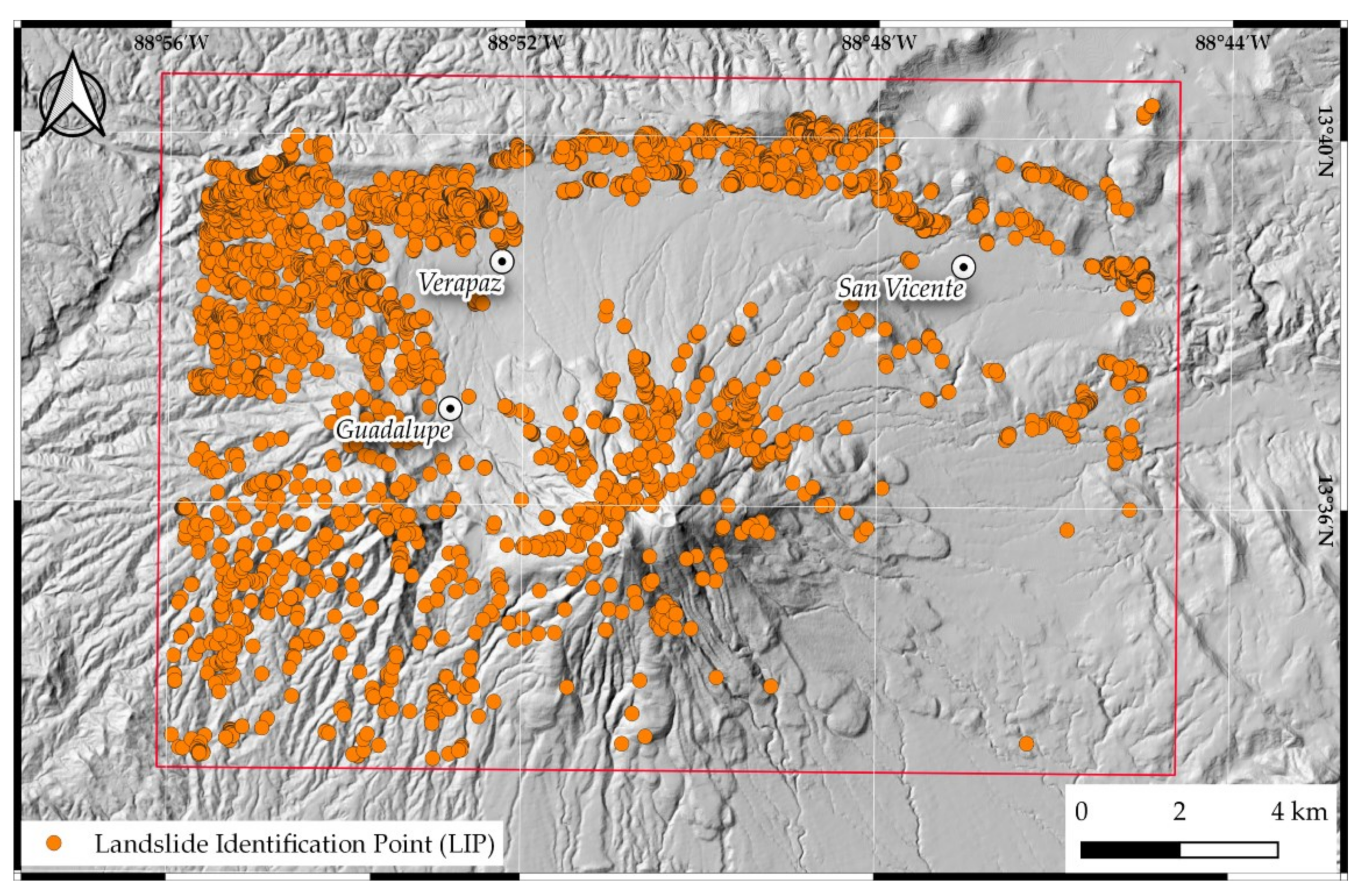
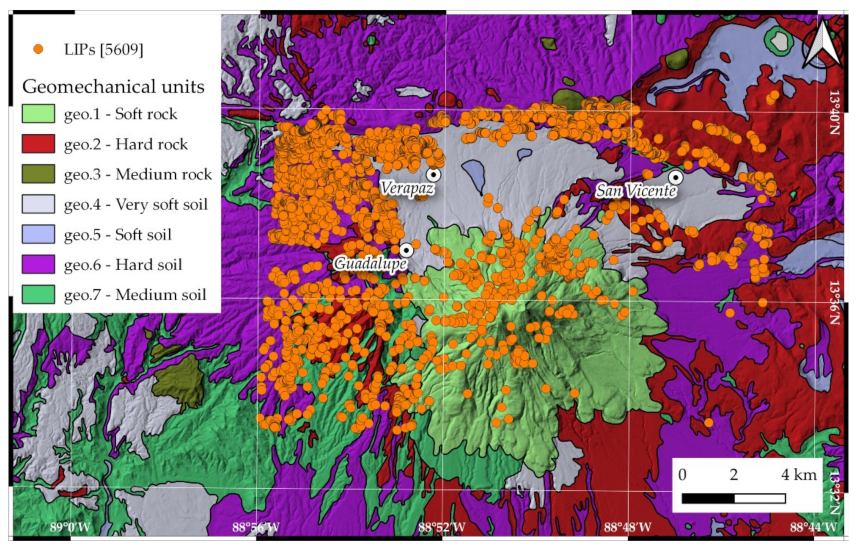
The visual analysis of the Google Earth images dated 21 November 2009 and available for the study area allowed us to identify 5609 LIPs relative to the debris flows triggered by the paroxysmal event happened on 7 and 8 November 2009 (Figure 5). LIPs are mainly located in the northern, western, and north-western sectors of the study area, as well as in the slopes of the San Vicente volcano. Almost half (i.e., 2753) of the LIPs are located over the hard soil unit (Figure 6), which includes acid pyroclastic rocks and volcanic epiclastites, being the class with the greatest areal extension (Table 1). The second highest frequency of LIPs (i.e., 979) is observed for the Tierra Blanca unit, which includes acidic pyroclastites and subordinate volcanic epiclastites and acid effusive rocks (geo.4). The class geo.1 (intermediate basic effusive rocks and subordinate pyroclastites), which is the second largest lithological unit, hosts 612 LIPs, representing around the 11% of the LIPs’ inventory.

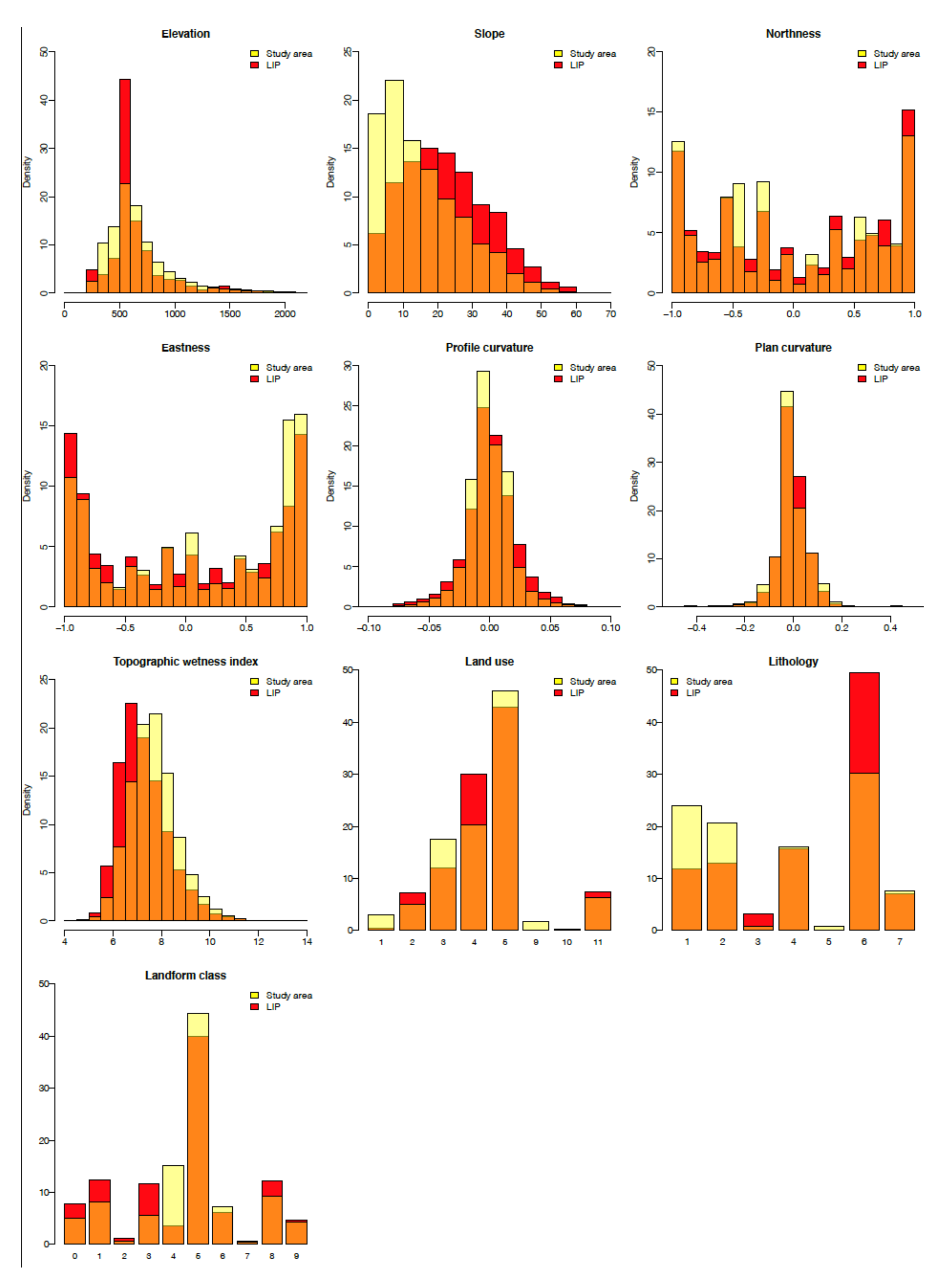
Figure 7 shows the relative frequency distributions [%] of the selected predictors calculated over the entire study area and only on the pixels intersecting one or more LIPs (i.e., positive pixels). Different distributions of a predictor observed in the entire area and where LIPs occur are expected to indicate a relationship between the spatial variability of that predictor and the LIPs’ positions. On the other hand, similar distributions should suggest no correlation between predictor and target variable. The distributions of elevation share the same center, but that observed on positive pixels is clearly less dispersed, indicating that pixels in the range 500–600 m asl are more likely to host a LIP. The slope frequency distribution observed on positive pixels is centered at a higher steepness than that observed on the entire area, reflecting that debris flows are more likely to start on pixels with slope angle between 10 and 30°. Frequency distributions of northness and eastness reflect the distribution of the LIPs over the study area (Figure 5), which occur more frequently on slopes facing east and north. Frequency distributions of plan and profile curvature calculated on the entire dataset and on positive pixels appear very similar, whereas those of TWI are differently skewed revealing that LIPs occur more frequently at low to moderate values and thus on the middle and upper portions of the slopes. Frequency distributions of USE and LCL show small to moderate differences, whereas those of GEO indicate that hard soil (geo.6) is the lithology class most prone to debris flows and soft (geo.1) and hard (geo.2) rocks are the most stable.

3.2. Calibration and Validation of the Models

Calibration and validation of MARS models were performed by using all the selected environmental variables as predictors. The variance inflation factor (VIF), indeed, which is below the threshold of ten for all the independent continuous variables, revealed absence of strong correlations among them (

Table 3. Variance Inflation Factor values calculated for the seven continuous variables.

VARIABLES	VIF
ELE	1.308
PLC	1.491
PRC	1.276
SLO	2.013
TWI	2.205
NORTH	1.003
EAST	1.035

).

The dataset employed to calibrate and validate the debris flows predictive models includes 2,794,399 pixels of 10 m, which cover the entire study area. 4975 of these pixels host one or more LIPs and are classified as “positive cells”. The remaining 2,789,424 pixels are classified as “negative cells”. The first step of the validation procedure consisted in preparing 100 random samples, including 1244 pixels (25% of the total positive cases) and the same number of negatives cases. Then, each of the 100 samples were split into a training and a test subset, both balanced in terms of positive and negative cases and including 75% and 25% of the 1244 pixels, respectively.

Figure 8 shows 100 ROC curves, each revealing the fit of a MARS model to a test subset, as well as the average ROC curve. The latter achieves an AUC value of 0.80, which reflects excellent predictive performance of the MARS models. Moreover, the standard deviation of the 100 AUC values, which is equal to 0.01, demonstrates the robustness of the procedure to changes of the learning and validation samples.

The average ROC curve was employed to calculate the Youden’s index J, which is equal to 0.46 and represents the optimal cut-off value allowing to maximize the sum of sensitivity and specificity. This value was employed to calculate an average confusion matrix for all of the 100 random samples of 2488 pixels, with a 1:1 ratio of positive-to-negative instances, as well as for the entire dataset, which has a high prevalence of negative pixels (

Table 4. Validation results for the balanced and all-area Multivariate Adaptive Regression Splines (MARS) models.

MODELS	N° PIXELS	CUT-OFF	POSITIVE CASES	NEGATIVE CASES	TP	FP	TN	FN
Balanced	2488	0.46	1244	1244	985	417	827	259
All-area	2,794,399	0.46	4975	2,789,424	3992	933,454	1,855,970	983
MODELS	ACCURACY	SENSITIVITY	SPECIFICITY	PPV	NPV	AUC
Balanced	0.73	0.79	0.66	0.70	0.76	0.80
All-area	0.67	0.80	0.67	0.00	0.99	0.81

).

Sensitivity of the 100 model runs (balanced models) and that calculated for the average probability values computed for all the pixels of the area (all-area model) is 0.79 and 0.80, respectively, demonstrating a good predictive skill of event pixels; on the other hand, specificity values are 0.66 and 0.67, respectively, thus reflecting a lower ability of the MARS models to detect true negatives. The accuracy of the balanced models (0.73) is substantially higher than that achieved by the all-area model (0.67), due to the very high number of false positives (FP) predicted over the entire dataset. Positive predictive value (PPV) and negative predictive value (NPV), which are calculated as TP/(TP + FP) and TN/(TN + FN), are 0.70 and 0.76 for the balanced models, whereas they are 0.00 and 0.99 when computed on the entire study area. The values of PPV and NPV calculated for the all-area model reflect the high number of FP and the high ratio of TN to FN, respectively.

The AUC value (0.81) achieved by the all-area model, also reported in Table 4, indicates, in accordance with the classification proposed by Hosmer and Lemeshow [56], an excellent ability of the predictive model to discriminate between observed presences and absences.

Figure 9 displays the relative importance of the predictor variables assessed by using the nsubsets criterion [9,35,54]. Slope is the most important independent variable, followed by three classes of GEO (i.e., geo.1, geo.2 and geo.7) and LCL (i.e., lcl.3, lcl.4 and lcl.5), and by ELE, which achieve a relative importance higher than 30%.

3.3. Landslide Susceptibility Map

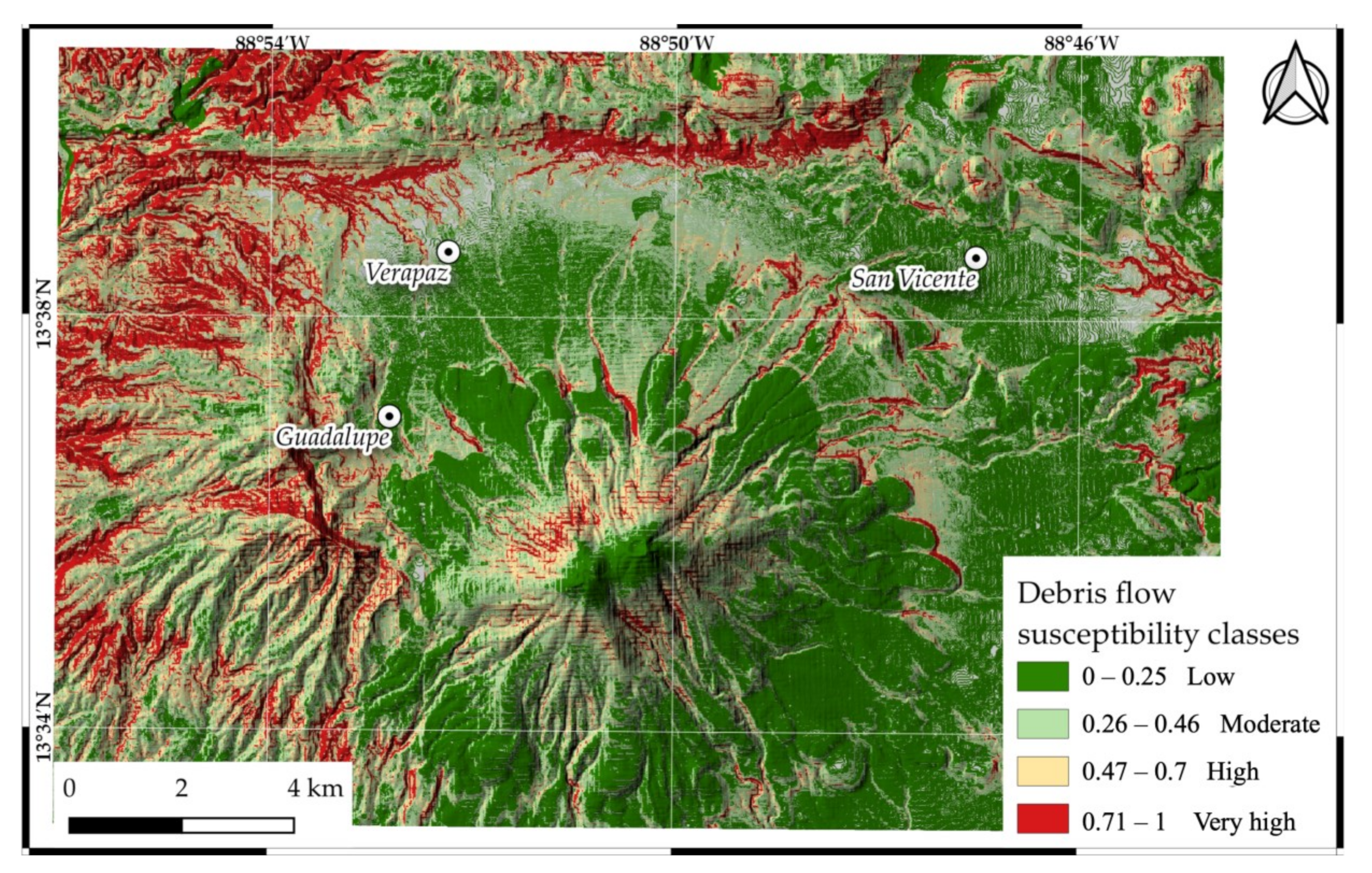
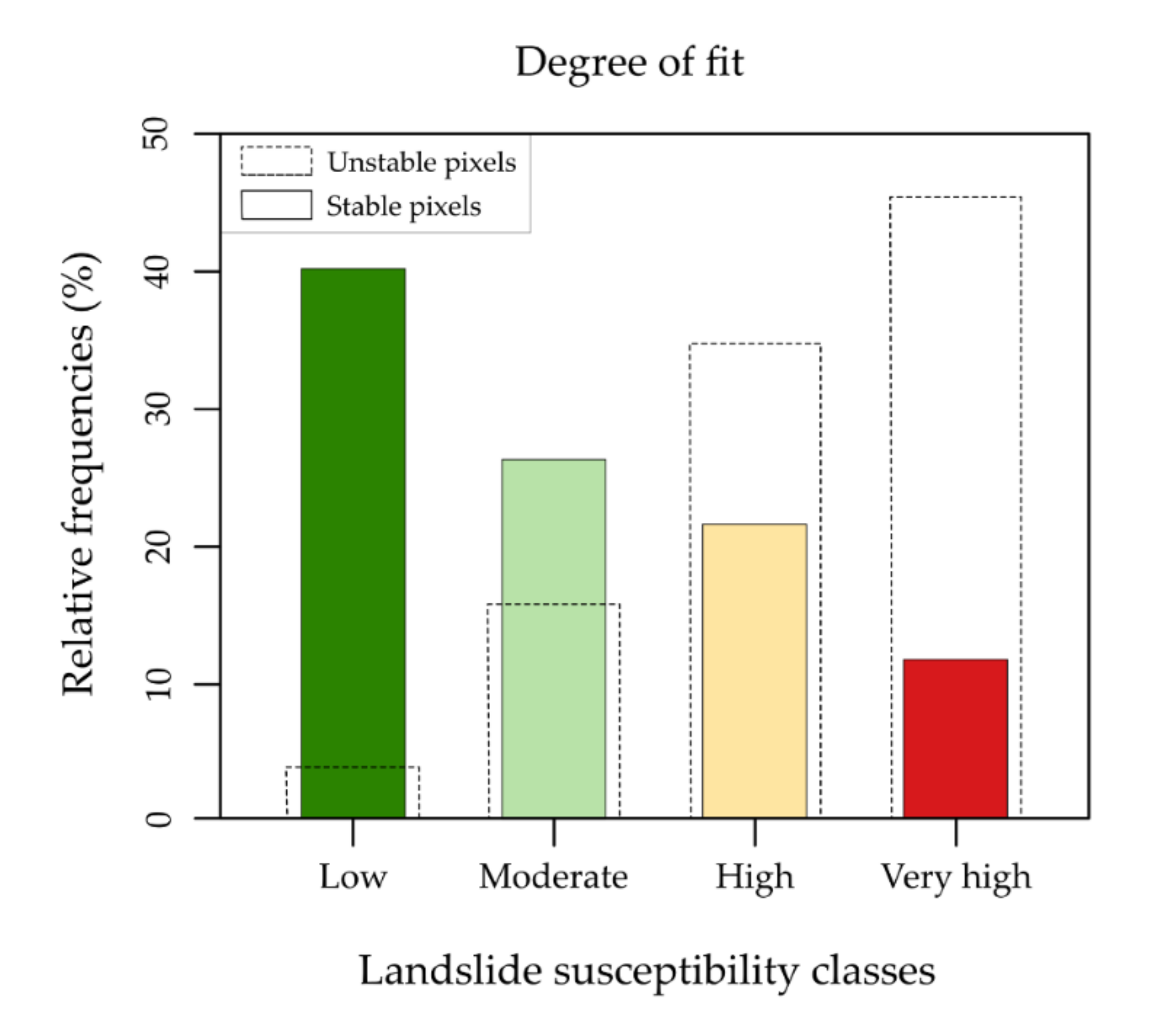
Figure 10 shows the final debris flow susceptibility map, obtained by averaging the probability values calculated by the 100 MARS model runs for each of the 2,794,399 pixels of the study area. The map was created by classifying the probability values into four levels, according to the optimal cut-off value J (0.46) and the subsequent two different Youden’s indexes (equal to 0.25 and 0.7, respectively) calculated to discriminate very low/low and high/very high susceptibility levels. The “degree of fit” between the susceptibility map and the spatial distribution of the LIPs is shown in Figure 11. The latter reveals that the frequency of the probability classes decreases from the lowest to the highest levels, whereas frequency of LIPs shows an inverse trend achieving the highest value in the highest susceptibility class.

4. Discussion and Conclusions

In this experiment, susceptibility to debris flow initiation in the area of the San Vicente volcano (El Salvador, CA) was evaluated by preparing an inventory including thousands of landslides triggered by heavy rainfalls due to the Hurricane Ida and the 96E low-pressure system (November 2009) and by modelling the relationship between the location of these landslides and the spatial variability of a set of environmental variables by using MARS as a modelling technique.

The validation of the MARS models, which was performed on 100 random samples of pixels, revealed an overall excellent ability to predict the debris flows that occurred in the San Vicente area, as attested by an average AUC value equal to 0.80. Moreover, the very low standard deviation of AUC values (0.01) demonstrated the robustness of the modelling procedure, which achieved very similar performance when changing the learning and validation samples. The cut-off dependent metrics, which were calculated by applying the Youden’s index as threshold to discriminate between pixels predicted as positives and negatives, revealed a different ability of the models to identify event (sensitivity = 0.79) and stable (specificity = 0.66) cells. This difference in performance reflects a relatively low number of false negatives, on the one hand, and a high number of false positives on the other. The number of false positives increases proportionally when the model is applied to the entire study area (i.e., all-area model). This data indicates that the model tends to overestimate the susceptibility to debris flows in the area of San Vicente. However, it is worth noting that an excess of false positives constitutes a less serious prediction error than that due to a large number of false negatives. In fact, while landslides could occur in the future in pixels erroneously predicted as unstable, those pixels that have been considered stable and where landslides have occurred constitute an irreversible error. Besides, in light of the geomorphological setting of the area and its high exposure to severe rainfall triggering events, false positive cases are to be considered as potential future initiation points.

The ability of MARS to predict debris flow source sites in the San Vicente area is very similar to that measured in the Ilopango Caldera, El Salvador [34,35], by using an inventory of landslides also triggered by the Hurricane Ida and the 96E low-pressure system (AUC = 0.81–0.82; Std. dev. = 0.006). The performance of MARS observed in this study is slightly better than that evaluated by Vargas et al. [36] in Mocoa (Colombia) with debris flows triggered by a heavy rainfall event, where average AUC was 0.78, but with a very low standard deviation (0.007). Regarding the threshold dependent metrics, similar values of sensitivity (0.84) and specificity (0.66) were found in the area of the Ilopango Caldera by Rotigliano et al. [34,35]. The specificity values also found in these previous studies indicate that future research should address the issue of the high number of false positives generated by the MARS model.

The evaluation of the importance of the predictor variables revealed that slope angle (SLO) and elevation (ELE) are the most important continuous predictors, whereas, among the categorical variables, three classes of lithology (GEO) and landform classification (LCL) achieved a high relative importance (>30%). The analysis of the variables’ importance, which was based on the nsubsets criterion, partially confirms what can be inferred from the comparison of the variables’ relative frequency distributions observed on the entire area and on the positive pixels (Figure 7). These distributions are indeed somewhat different for SLO and ELE, but also for TWI, EAST, and NORTH, which instead exhibited low importance (<20%). Based on the high density of LIPs, we would have expected a high importance of the lithology category geo.6 (hard soil), whose relative contribution to the MARS models is, however, very low. This result confirms the ability of the multivariate statistical approach to recognize and recall the role of really important variables, which are also coherent and adequate in terms of geomorphological modelling.

A strong relationship between landslide locations and variability of slope angle and elevation was also found in other landslide susceptibility studies that employed MARS as modelling techniques [34,36]. Regarding the Ilopango Caldera area, Rotigliano et al. [35] calculated a high importance for elevation and terrain ruggedness index. The latter variable is usually strongly correlated with slope steepness, thus we can infer that the importance of the continuous predictors of debris flows is somewhat similar in the two areas of El Salvador. On the other hand, the analysis of the importance of the categorical variables revealed different results, as GEO and LCL exhibited low importance in the Ilopango Caldera area, whereas a relatively strong relationship was found between some of the USE classes and the location of debris flows.

On the basis of the results obtained in this experiment, the following conclusions can be drawn for the area of San Vicente volcano (El Salvador, CA):

• The MARS technique confirms its ability in modelling debris flow susceptibility in volcanic steep slopes, being able to predict the locations of debris flows with excellent accuracy (AUC = 0.80) by using a set of environmental variables that can be extracted from available thematic maps and a DEM with 10-m horizontal resolution as predictors;
• The ability of MARS to predict the spatial distribution of debris flows is stable when changes of the learning and validation samples are performed (AUC Std. dev. = 0.01);
• The cut-off dependent metrics revealed that MARS models produce a large number of false positives, and thus their ability to identify stable cells is moderate (specificity = 0.66);
• MARS exhibits the same predictive skill in the San Vicente area as that achieved in other study areas located in El Salvador and Colombia;
• MARS modelling revealed that slope angle, elevation, lithology, and landform classification are the most important predictors of the debris flows occurred in the study area.

The modeling procedure described in this paper allow for preparing debris flow susceptibility maps by using data typically available on a large scale. In contrast to the previous study [23], which was based on a deterministic approach, the map we obtained depicts the susceptibility to debris flow initiation in a large sector of the San Vicente area, without depending on the actual respondence of local shallow to deep setting to the one hypothesized in 2D modelling; however, according to the factor importance analysis, the statistical model largely fits with physically sound failure mechanisms. At the same time, the pixels in the susceptibility map with high scores could be taken as an input for physical modelling as more likely initiation points.

In light of the adopted calibration event and modelling method, we can consider the susceptibility map obtained as accurate in reproducing the expected landslide initiation scenario driven by a triggering event having a magnitude similar to the one of 2009. As Ida hurricane-like phenomena are recurrent in El Salvador, investigating and optimizing susceptibility modelling and mapping is of a great importance. In fact, predictive maps may help land planners and environmental agencies in adopting actions aimed to mitigate landslide risk and avoid severe damages or even casualties caused by their occurrence in urbanized areas. At the same time, the susceptibility model and map obtained, which were optimized for detecting the initiation points for future debris flow phenomena, are the basis for the now running step of this research aimed at the implementation of a propagation routing algorithm so to produce a full predictive scenario. Both initiation and propagation predictive scenario maps are in fact mandatory for converting a weather fore/now-cast into an effective early warning system.

References

1. Rose, W.I.; Bommer, J.J.; López, D.L.; Carr, M.J.; Major, J.J. Natural Hazards in El Salvador; Geological Society of America Boulder: Boulder, CO, USA, 2004. [Google Scholar]
2. Depresión Tropical 12E/Sistema Depresionario Sobre El Salvador y Otros Eventos Extremos del Pacífico—El Salvador. Available online: https://reliefweb.int/report/el-salvador/depresión-tropical-12e-sistema-depresionario-sobre-el-salvador-y-otros-eventos (accessed on 16 January 2020).
3. Crone, A.J.; Baum, R.L.; Lidke, D.J.; Sather, D.N.; Bradley, L.-A.; Tarr, A.C. Landslides Induced by Hurricane Mitch in El Salvador—An Inventory and Descriptions of Selected Features; Geological Society of America: Boulder, CO, USA, 2001. [Google Scholar]
4. Larsen, M.C.; Wieczorek, G.F. Geomorphic effects of large debris flows and flash floods, northern Venezuela, 1999. Z. Fur Geomorphol. Suppl. 2006, 145, 147–175. [Google Scholar]
5. Larsen, M.C. Rainfall-triggered landslides, anthropogenic hazards, and mitigation strategies. Adv. Geosci. 2008. [Google Scholar] [CrossRef] [Green Version]
6. Avelar, A.S.; Netto, A.L.C.; Lacerda, W.A.; Becker, L.B.; Mendonça, M.B. Mechanisms of the recent catastrophic landslides in the mountainous range of Rio de Janeiro, Brazil. In Landslide Science and Practice: Global Environmental Change; Avelar, A.S., Netto, A.L.C., Lacerda, W.A., Becker, L.B., Mendonça, M.B., Eds.; Springer: Berlin/Heidelberg, Germany, 2013. [Google Scholar]
7. Hungr, O.; Leroueil, S.; Picarelli, L. The Varnes classification of landslide types, an update. Landslides 2014, 11, 167–194. [Google Scholar] [CrossRef]
8. Brabb, E. Innovative Approaches for Landslide Hazard Evaluation. In Proceedings of the IV International Symposium on Landslides, Toronto, ON, Canada, 16–21 September 1984; pp. 307–323. [Google Scholar]
9. Conoscenti, C.; Rotigliano, E.; Cama, M.; Caraballo-Arias, N.A.; Lombardo, L.; Agnesi, V. Exploring the effect of absence selection on landslide susceptibility models: A case study in Sicily, Italy. Geomorphology 2016, 261, 222–235. [Google Scholar] [CrossRef]
10. Reichenbach, P.; Rossi, M.; Malamud, B.D.; Mihir, M.; Guzzetti, F. A review of statistically-based landslide susceptibility models. EarthSci. Rev. 2018, 180, 60–91. [Google Scholar] [CrossRef]
11. Carrara, A.; Agnesi, V.; Macaluso, T.; Monteleone, S.; Pipitone, G. Slope movements induced by the Southern Italy earthquake of November 1980. IAEG 1986, 2, 237–250. [Google Scholar]
12. Agnesi, V.; Carrara, A.; Macaluso, T.; Monteleone, S.; Pipitone, G.; Sorriso-Valvo, M. Elementi tipologici e morfologici dei fenomeni di instabilità dei versanti indotti dal sisma del 1980 (alta Valle del Sele). Geol. Appl. e Idrogeol. 1983, 18, 309–341. [Google Scholar]
13. Chung, C.-J.F.; Fabbri, A.G. Validation of Spatial Prediction Models for Landslide Hazard Mapping. Nat. Hazards 2003, 30, 451–472. [Google Scholar] [CrossRef]
14. Chung, C.J.; Fabbri, A.G. Predicting landslides for risk analysis—Spatial models tested by a cross-validation technique. Geomorphology 2008, 94, 438–452. [Google Scholar] [CrossRef]
15. Guzzetti, F.; Carrara, A.; Cardinali, M.; Reichenbach, P. Landslide hazard evaluation: A review of current techniques and their application in a multi-scale study, Central Italy. Geomorphology 1999, 31, 181–216. [Google Scholar]
16. Guzzetti, F.; Reichenbach, P.; Cardinali, M.; Galli, M.; Ardizzone, F. Probabilistic landslide hazard assessment at the basin scale. Geomorphology 2005, 72, 272–299. [Google Scholar] [CrossRef]
17. Guzzetti, F.; Reichenbach, P.; Ardizzone, F.; Cardinali, M.; Galli, M. Estimating the quality of landslide susceptibility models. Geomorphology 2006, 81, 166–184. [Google Scholar] [CrossRef]
18. Clerici, A.; Perego, S.; Tellini, C.; Vescovi, P. A GIS-based automated procedure for landslide susceptibility mapping by the Conditional Analysis method: The Baganza valley case study (Italian Northern Apennines). Environ. Geol. 2006, 50, 941–961. [Google Scholar] [CrossRef]
19. Conoscenti, C.; Di Maggio, C.; Rotigliano, E. GIS analysis to assess landslide susceptibility in a fluvial basin of NW Sicily (Italy). Geomorphology 2008. [Google Scholar] [CrossRef]
20. Costanzo, D.; Rotigliano, E.; Irigaray, C.; Jiménez-Perálvarez, J.D.; Chacón, J. Factors selection in landslide susceptibility modelling on large scale following the gis matrix method: Application to the river Beiro basin (Spain). Nat. Hazards Earth Syst. Sci. 2012, 12, 327–340. [Google Scholar] [CrossRef]
21. Rotigliano, E.; Cappadonia, C.; Conoscenti, C.; Costanzo, D.; Agnesi, V. Slope units-based flow susceptibility model: Using validation tests to select controlling factors. Nat. Hazards 2012, 61, 143–153. [Google Scholar] [CrossRef]
22. Verstappen, H.T. Geomorphology of the Agri valley, southern Italy. ITC J. 1983, 4, 291–301. [Google Scholar]
23. Smith, D.M.; Oommen, T.; Bowman, L.J.; Gierke, J.S.; Vitton, S.J. Hazard assessment of rainfall-induced landslides: A case study of San Vicente volcano in central El Salvador). Nat. Hazards 2015, 75, 2291–2310. [Google Scholar] [CrossRef]
24. Cruden, D.M.; Varnes, D.J. Landslide Types and Processes. In Landslides Investigation and Mitigation, Transportation Research Board, Special Report No. 247; Turner, A.K., Shuster, R.L., Eds.; National Academic Press: Washington. DC, USA, 1996; pp. 36–75. Available online: http://onlinepubs.trb.org/Onlinepubs/sr/sr247/sr247.pdf (accessed on 16 January 2020).
25. Sassa, K.; Wang, G.H. Mechanism of landslide-triggered debris flows: Liquefaction phenomena due to the undrained loading of torrent deposits. In Debris-Flow Hazards and Related Phenomena; Springer: Berlin/Heidelberg, Germany, 2007; pp. 81–104. [Google Scholar]
26. Friedman, J.H. Multivariate Adaptive Regression Splines. Ann. Stat. 1991, 19, 1–67. [Google Scholar] [CrossRef]
27. Gutiérrez, Á.G.; Schnabel, S.; Lavado Contador, J.F. Using and comparing two nonparametric methods (CART and MARS) to model the potential distribution of gullies. Ecol. Modell. 2009, 220, 3630–3637. [Google Scholar] [CrossRef]
28. Gómez-Gutiérrez, Á.; Conoscenti, C.; Angileri, S.E.; Rotigliano, E.; Schnabel, S. Using topographical attributes to evaluate gully erosion proneness (susceptibility) in two mediterranean basins: Advantages and limitations. Nat. Hazards 2015, 79, 291–314. [Google Scholar] [CrossRef]
29. Conoscenti, C.; Agnesi, V.; Cama, M.; Caraballo-Arias, N.A.; Rotigliano, E. Assessment of Gully Erosion Susceptibility Using Multivariate Adaptive Regression Splines and Accounting for Terrain Connectivity. L. Degrad. Dev. 2018, 29, 724–736. [Google Scholar] [CrossRef]
30. Conoscenti, C.; Rotigliano, E. Predicting gully occurrence at watershed scale: Comparing topographic indices and multivariate statistical models. Geomorphology 2020, 359. [Google Scholar] [CrossRef]
31. Conoscenti, C.; Angileri, S.; Cappadonia, C.; Rotigliano, E.; Agnesi, V.; Märker, M. Gully erosion susceptibility assessment by means of GIS-based logistic regression: A case of Sicily (Italy). Geomorphology 2014, 204, 399–411. [Google Scholar] [CrossRef] [Green Version]
32. Conoscenti, C.; Ciaccio, M.; Caraballo-Arias, N.A.; Gómez-Gutiérrez, Á.; Rotigliano, E.; Agnesi, V. Assessment of susceptibility to earth-flow landslide using logistic regression and multivariate adaptive regression splines: A case of the Belice River basin (western Sicily, Italy). Geomorphology 2015, 242, 49–64. [Google Scholar] [CrossRef]
33. Garosi, Y.; Sheklabadi, M.; Pourghasemi, H.R.; Besalatpour, A.A.; Conoscenti, C.; Van Oost, K. Comparison of differences in resolution and sources of controlling factors for gully erosion susceptibility mapping. Geoderma 2018, 330, 65–78. [Google Scholar] [CrossRef]
34. Rotigliano, E.; Martinello, C.; Agnesi, V.; Conoscenti, C. Evaluation of debris flow susceptibility in El Salvador (CA): A comparisobetween multivariate adaptive regression splines (MARS) and binary logistic regression (BLR). Hungarian Geogr. Bull. 2018, 67, 361–373. [Google Scholar] [CrossRef] [Green Version]
35. Rotigliano, E.; Martinello, C.; Hernandéz, M.A.; Agnesi, V.; Conoscenti, C. Predicting the landslides triggered by the 2009 96E/Ida tropical storms in the Ilopango caldera area (El Salvador, CA): Optimizing MARS-based model building and validation strategies. Environ. Earth Sci. 2019, 78. [Google Scholar] [CrossRef]
36. Vargas-Cuervo, G.; Rotigliano, E.; Conoscenti, C. Prediction of debris-avalanches and -flows triggered by a tropical storm by using a stochastic approach: An application to the events occurred in Mocoa (Colombia) on 1 April 2017. Geomorphology 2019, 339, 31–43. [Google Scholar] [CrossRef]
37. Carrara, A.; Crosta, G.; Frattini, P. Comparing models of debris-flow susceptibility in the alpine environment. Geomorphology 2008. [Google Scholar] [CrossRef]
38. Van Den Eeckhaut, M.; Reichenbach, P.; Guzzetti, F.; Rossi, M.; Poesen, J. Combined landslide inventory and susceptibility assessment based on different mapping units: An example from the Flemish Ardennes, Belgium. Nat. Hazards Earth Syst. Sci. 2009. [Google Scholar] [CrossRef] [Green Version]
39. Costanzo, D.; Chacón, J.; Conoscenti, C.; Irigaray, C.; Rotigliano, E. Forward logistic regression for earth-flow landslide susceptibility assessment in the Platani river basin (southern Sicily, Italy). Landslides 2014, 11, 639–653. [Google Scholar] [CrossRef] [Green Version]
40. Lombardo, L.; Cama, M.; Maerker, M.; Rotigliano, E. A test of transferability for landslides susceptibility models under extreme climatic events: Application to the Messina 2009 disaster. Nat. Hazards 2014, 74, 1951–1989. [Google Scholar] [CrossRef]
41. Cama, M.; Conoscenti, C.; Lombardo, L.; Rotigliano, E. Exploring relationships between grid cell size and accuracy for debris-flow susceptibility models: A test in the Giampilieri catchment (Sicily, Italy). Environ. Earth Sci. 2016, 75, 1–21. [Google Scholar] [CrossRef]
42. Major, J.J.; Schilling, S.P.; Pullinger, C.R.; Escobar, C.D.; Howell, M.M. USGS Open-File Report 01-367: Volcano-Hazard Zonation for San Vicente Volcano, El Salvador. Available online: https://pubs.usgs.gov/of/2001/0367/ (accessed on 16 November 2020).
43. Avila, L.A.; Cangialosi, J. Tropical Cyclone Report: Hurricane Ida; National Hurricane Center: Miami, FL, USA, 2010. Available online: https://www.nhc.noaa.gov/data/tcr/AL112009_Ida.pdf (accessed on 16 November 2020).
44. Avila, R. Síntesis de los Informes de Evaluación Técnica de las Lluvias del 7 y 8 de Noviembre 2009 en El Salvador: Análisis del impacto Físico Natural y Vulnerabilidad Socio Ambiental; report Comisión Técnico Científica; Coordina el Ministerio de Medio Ambiente y Recursos Naturales, MARN: San Salvador, El Salvador, 2010; Available online: https://www.academia.edu/42170439/_Síntesis_de_los_informes_de_evaluación_técnica_de_las_lluvias_del_7_y_8_de_noviembre_2009_en_El_Salvador_Análisis_del_impacto_físico_natural_y_vulnerabilidad_socio_ambiental_ (accessed on 16 November 2020).
45. Rotigliano, E.; Agnesi, V.; Cappadonia, C.; Conoscenti, C.; Agnesi, V. The role of the diagnostic areas in the assessment of landslide susceptibility models: A test in the sicilian chain. Nat. Hazards 2011, 58, 981–999. [Google Scholar] [CrossRef]
46. Cama, M.; Lombardo, L.; Conoscenti, C.; Agnesi, V.; Rotigliano, E. Predicting storm-triggered debris flow events: Application to the 2009 Ionian Peloritan disaster (Sicily, Italy). Nat. Hazards Earth Syst. Sci. 2015, 15, 1785–1806. [Google Scholar] [CrossRef] [Green Version]
47. Conrad, O.; Bechtel, B.; Bock, M.; Dietrich, H.; Fischer, E.; Gerlitz, L.; Wehberg, J.; Wichmann, V.; Böhner, J. System for Automated Geoscientific Analyses (SAGA) v. 2.1.4. Geosci. Model Dev. 2015, 8, 1991–2007. [Google Scholar] [CrossRef] [Green Version]
48. Weber, H.S.; Wiesemann, G.; Lorenz, W.; Schmidt-Thomé, M. Mapa Geológico de la República de El Salvador/América Central = Geologische Karte der Republik El Salvador/Mittelamerika. Available online: https://nla.gov.au/nla.obj-726140200/view (accessed on 16 November 2020).
49. Ohlmacher, G.C. Plan curvature and landslide probability in regions dominated by earth flows and earth slides. Eng. Geol. 2007, 91, 117–134. [Google Scholar] [CrossRef]
50. Allison, P.D. Logistic Regression Using the SAS System: Theory and Application; SAS Institute Inc.: Cary, NC, USA. Available online: http://www.sciepub.com/reference/248083 (accessed on 16 November 2020).
51. Hair, J.; Black, W.; Babin, B.; Anderson, R. Multivariate Data Analysis: A Global Perspective: Pearson Education International; Pearson Education: Upper Saddle River, NJ, USA; London, UK, 2010. [Google Scholar]
52. Keith, T.Z. Multiple Regression and Beyond; Routledge: Milton Park, Abingdon, UK, 2014. [Google Scholar]
53. Naimi, B. Uncertainty analysis for species distribution models. R Softw. Packag. 2015. [Google Scholar] [CrossRef]
54. Martinello, C.; Cappadonia, C.; Conoscenti, C.; Agnesi, V.; Rotigliano, E. Optimal slope units partitioning in landslide susceptibility mapping. J. Maps 2020. [Google Scholar] [CrossRef]
55. Milborrow, S. Notes on the Earth Package. 2020. Available online: http://www.milbo.org/doc/earth-notes.pdf (accessed on 16 November 2020).
56. Hosmer, D.W.; Lemeshow, S. Applied Logistic Regression; John Wiley & Sons, Inc.: Hoboken, NJ, USA, 2000; ISBN 9780471722144. [Google Scholar]
57. Youden, W.J. Index for rating diagnostic tests. Cancer 1950, 3, 32–35. [Google Scholar] [CrossRef]
58. Cama, M.; Lombardo, L.; Conoscenti, C.; Rotigliano, E. Improving transferability strategies for debris flow susceptibility assessmentApplication to the Saponara and Itala catchments (Messina, Italy). Geomorphology 2017, 288, 52–65. [Google Scholar] [CrossRef]
Figure 1. Location of the study area. This is located in the central sector of El Salvador, Central America (a); within the area under study (b) there are 3 towns: Guadalupe, Verapaz and San Vicente (c).
Earth 02 00005 g001
Figure 2. These two false color images generated by the Advanced Spaceborne Thermal Emission and Reflection Radiometer (ASTER) on NASA’s TERRA show the area under examination (see Figure 1 for the location) before (a) and after (b) the event of 7 and 8 November 2009. The images were prepared with artificial colors to make the vegetation (in red) distinguishable from the bare ground (in gray). NASA Earth Observatory image by Robert Simmon, based on data from the NASA/GSFC/METI/ERSDAC/JAROS, and U.S./Japan ASTER Science Team, https://earthobservatory.nasa.gov/images/41365/landslides-on-volcan-de-san-vicente.
Earth 02 00005 g002
Figure 3. An area hit by a debris flow in Verapaz after the simultaneous action of Hurricane Ida and the low-pressure system 96E. Photo by Yuri Cortez, 9 November 2009. AFP/Getty Images, https://volcano.si.edu/volcano.cfm?vn=343070. Large blocks entrained into the debris flows propagated floating on the surge invading a road.
Earth 02 00005 g003
Figure 4. Geological map of the study area (see Table 1 for the lithologic description).
Earth 02 00005 g004
Figure 5. Map of the 5609 landslide identification points (LIPs) identified in the study area.
Earth 02 00005 g005
Figure 6. Spatial distribution of the 5609 LIPs over the lithological map.
Earth 02 00005 g006
Figure 7. Relative frequency distributions [%] of the selected predictors calculated over the entire study area (yellow) and only on the pixels intersecting one or more LIPs (red). Orange is for overlapping boxes.
Earth 02 00005 g007
Figure 8. Receiver operating characteristic (ROC) curves processed using the MARS method in the study area.
Earth 02 00005 g008
Figure 9. Relative importance of the predictor variables. Thicker lines and bigger circles indicate importance higher than 30%.
Earth 02 00005 g009
Figure 10. Debris flow susceptibility map of the study area.
Earth 02 00005 g010
Figure 11. Relative frequency distributions of the debris flow susceptibility levels (solid outline) and of the LIPs (dotted outlines) calculated for the four levels.
Earth 02 00005 g011