A Hybrid Quantum–Classical Variational Linear Solver for Power Flow Analysis in Smart Grids with V2G Integration

Abstract

This paper presents a simulation-based proof of concept for integrating an existing Variational Quantum Linear Solver (VQLS) with a Newton-type AC power flow procedure for smart grids with vehicle-to-grid (V2G) participation. The novelty of the work lies not in proposing a new VQLS algorithm but in its engineering integration with a reduced Jacobian-based power flow subproblem and V2G operating scenarios. The proposed framework linearizes the nonlinear AC power flow equations and applies a four-qubit Real-Amplitudes VQLS circuit with the COBYLA optimizer to approximate a selected 16 × 16 reduced Jacobian system. The complete voltage profile is then reconstructed through the hybrid quantum–classical procedure. The method is evaluated using a modified IEEE 33-bus radial distribution system with an aggregated V2G unit connected at Bus 18. The main optimization run shows a rapid reduction and subsequent stabilization of the VQLS cost, while the resulting bus-voltage profile follows the overall trend of the Newton–Raphson reference solution. A separate 50-iteration assessment also reduces the cost substantially but does not reach the reference tolerance of 10⁻⁴. The V2G scenario analysis shows that prescribed V2G active-power support can reduce active power losses under both normal and stressed operating conditions, with loss reductions of 26.26%, 27.85%, and 30.52% in the base peak-load, N-1 contingency support, and dynamic railway-peak support cases, respectively. A resource-scaling assessment using a normalized classical computation index and a VQLS circuit-depth index is included only to illustrate resource-growth trends, not to establish computational superiority. The results support the feasibility of the proposed integration under ideal statevector simulation, but no quantum speedup or advantage over established classical solvers is claimed.

1. Introduction

Modern power systems are moving toward smart grid operation through the increasing use of renewable generation, distributed energy resources, battery energy storage systems, and electric vehicles (EVs). These technologies improve the flexibility of electricity supply and demand, but they also introduce variable generation, bidirectional power exchange, and more complex network operating conditions. Fang et al. [1] described the smart grid as an interconnected infrastructure in which communication, sensing, control, and distributed resources operate in coordination. Reliable power flow analysis therefore remains essential for evaluating bus voltages, active and reactive power flows, network losses, and operating limits.

Vehicle-to-grid (V2G) technology is an important part of this transition. Kempton and Tomić [2] established the concept of using aggregated EV batteries as controllable resources that can either draw power from or supply power to the grid. Later studies extended this idea to coordinated charging and energy management. Dankar et al. [3] developed a neural-network-based model predictive control strategy for a grid-connected photovoltaic–battery system with V2G and grid-to-vehicle operation. Li et al. [4] applied deep Q-learning to coordinate EV charging while allowing V2G participation. These developments show that EVs can act not only as electrical loads but also as flexible resources that support network operation.

The coordinated use of photovoltaic generation, battery storage, and EV charging has also been examined in microgrid and distribution-network applications. Thaitae et al. [5] evaluated a hybrid PV–battery energy storage system for an EV charging station in a microgrid. Chitgreeyan et al. [6] proposed a multi-period framework for controlling EV energy demand in an unbalanced power system while considering the spatial distribution of charging-station loads. Kongjeen et al. [7] modified the backward–forward sweep method to analyze microgrid load flow under different EV-load representations. Taken together, these studies indicate that EV integration can alter feeder loading, voltage profiles, and network losses, making coordinated energy management and accurate power flow analysis increasingly important.

Photovoltaic and battery storage resources have also been studied from the perspectives of sizing, placement, and system control. Prabpal et al. [8] optimized the size and location of battery energy storage using reactive-power control strategies. Chooseang et al. [9] examined photovoltaic sizing and placement with Volt–Var control and a unified power flow controller. Pengtem et al. [10] developed a multi-objective energy-management framework for a hybrid photovoltaic–hydropower–battery system serving remote communities. Rattanakam et al. [11] investigated battery sizing and placement for load-frequency control, whereas Deeum et al. [12] incorporated EV-load uncertainty into the robust optimization of photovoltaic and battery-storage configurations. These studies illustrate the need for computational approaches that can account for several distributed resources, uncertain EV demand, and changing network conditions.

Despite advances in optimization and control, conventional numerical methods remain the standard tools for power flow analysis. Tinney and Hart [13] introduced the Newton–Raphson power flow method, which is still widely used because of its strong convergence properties. Stott and Alsac [14] later developed the fast-decoupled load flow method to reduce the computational burden. Simplified formulations have also been proposed for specific applications, including the revised DC power flow model of Stott et al. [15] and the lossy DC formulation of Simpson-Porco [16]. Nevertheless, the convergence and accuracy of these methods remain influenced by network loading, topology, and matrix conditioning [17].

Open-source tools and standard benchmark systems have improved the reproducibility of power system studies. Thurner et al. [18] introduced Pandapower as a Python-based BSD-licensed version 1.4.3. Based platform for power flow, optimal power flow, short-circuit analysis, state estimation, and network optimization. Among commonly used benchmark networks, the IEEE 33-bus radial distribution system introduced by Baran and Wu [19] has been widely adopted for studies involving voltage regulation, loss reduction, network reconfiguration, distributed generation, and energy storage.

Classical solvers are effective for most present-day power system applications, but quantum computing provides another direction for addressing large linear-algebra and optimization problems. Deutsch [20] laid the theoretical foundation for universal quantum computation, while Nielsen and Chuang [21] established the broader framework of quantum information processing. Harrow, Hassidim, and Lloyd [22] subsequently introduced a quantum algorithm that prepares a quantum state proportional to the solution of a linear system. Childs et al. [23] later improved the dependence of quantum linear-system algorithms on solution precision.

Current quantum hardware still limits the practical implementation of these algorithms. Preskill [24] described present-day processors as noisy intermediate-scale quantum devices characterized by limited qubit counts, imperfect gate operations, and decoherence. Experimental progress has been demonstrated using programmable superconducting processors [25], but large-scale fault-tolerant quantum computation is not yet available. Hybrid quantum–classical algorithms have therefore attracted attention as a practical direction for near-term quantum applications [26].

Within this approach, the Variational Quantum Linear Solver (VQLS) introduced by Bravo-Prieto et al. [27] converts the solution of a linear system into a cost-function minimization problem. A parameterized quantum circuit produces a candidate solution, while a classical optimizer updates the circuit parameters. In the present study, the Constrained Optimization by Linear Approximation (COBYLA) algorithm is used because it can update the parameters without requiring analytical gradients.

Table 1. Summary of representative studies and their relationship to the present work.

Reference	Keywords	Relation to This Study
[2]	V2G, EV battery, bidirectional power	Foundation of V2G modeling
[3]	PV, BESS, MPC, V2G/G2V	Integrated EV-energy control
[4]	Deep Q-learning, EV charging, V2G	EV charging coordination
[5]	Microgrid, PV, BESS, EV station	Hybrid EV energy system
[6]	EV demand, optimization, unbalanced system	EV demand control
[7]	Load flow, BFS, EV model	Classical EV-integrated power flow
[8,9]	BESS, PV, sizing, Volt–Var	DER sizing and allocation
[10,11,12]	Energy management, uncertainty, optimization	Smart grid resource management
[13,14]	Newton–Raphson, FDLF	Classical power flow references
[22,23]	Quantum linear systems, HHL	Quantum linear-system foundations
[27]	VQLS, variational algorithm	Core quantum solution method
This work	VQLS, COBYLA, AC power flow, V2G	Hybrid quantum–classical power flow analysis

summarizes representative studies and their relationship to the present work.

Although previous studies have addressed EV charging coordination, V2G energy management, distributed-resource optimization, and classical load flow analysis, fewer studies have examined how an existing variational quantum linear solver can be embedded within a Newton-type AC power flow procedure for distribution-system analysis. It should be emphasized that the present work does not propose a new VQLS algorithm. The novelty lies in the engineering integration of the VQLS framework with a reduced Jacobian-based AC power flow formulation and in the assessment of its numerical behavior under V2G operating scenarios.

To make the scope of the quantum contribution explicit, the detailed IEEE 33-bus case study uses a four-qubit Real-Amplitudes circuit to represent a selected 16 × 16 reduced Jacobian subproblem. The remaining state variables are handled through the classical reconstruction stage. Therefore, the proposed method should be interpreted as a hybrid reduced-system implementation rather than a complete quantum solution of the full Newton–Raphson Jacobian for the IEEE 33-bus network.

To address this research gap, this study develops a hybrid quantum–classical framework for steady-state AC power flow analysis. At each power flow iteration, the nonlinear equations are linearized and expressed as a Jacobian-based linear system. The reduced system is supplied to the VQLS module, while COBYLA updates the parameters of the variational circuit by minimizing the residual-based cost function. The reconstructed correction vector is then returned to the classical power flow model to update the voltage magnitudes and phase angles.

The main evaluation uses a modified IEEE 33-bus radial distribution system with an aggregated EV-based V2G unit connected at Bus 18. The numerical study examines the VQLS cost trajectory, the bus-voltage profile relative to the Newton–Raphson reference solution, and the behavior of a separate fixed-budget convergence assessment. The voltage-profile comparison is intended to examine numerical consistency with the reference solution, not to claim exact equivalence or computational superiority.

The network-level assessment is extended to three prescribed V2G operating conditions: a base case without V2G support, a 20% V2G participation case, and a 50% V2G participation case. Their effects on active power losses are examined over a 24-h operating period. The term V2G participation in this study refers to prescribed steady-state operating scenarios rather than an optimized V2G dispatch schedule.

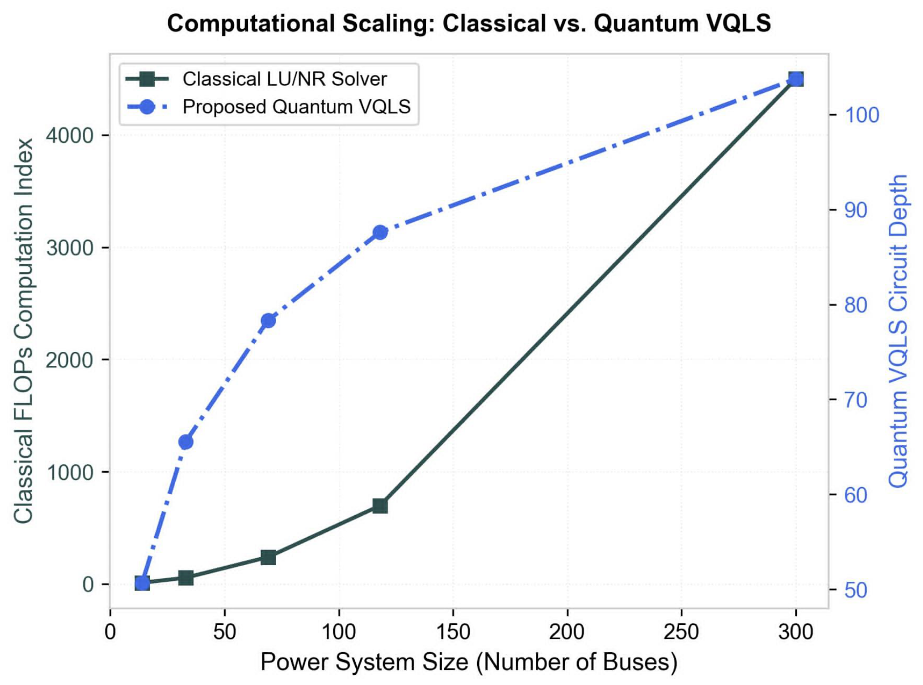
Preliminary resource-scaling trends are also evaluated for systems containing 14, 33, 70, 118, and 300 buses. The classical implementation is represented by a normalized classical computation index, whereas the VQLS implementation is represented by a circuit-depth index. Because these indicators describe different resources, they are used only to illustrate growth trends. They do not provide a direct execution-time comparison and do not establish quantum speedup or computational superiority over established classical solvers.

The principal contributions of this study are summarized as follows:

• A hybrid quantum–classical engineering framework is developed by embedding an existing VQLS formulation into a reduced Newton-type AC power flow procedure.
• A four-qubit VQLS implementation is applied to a selected 16 × 16 reduced Jacobian subproblem, while the complete voltage-profile calculation is recovered through classical reconstruction.
• The VQLS–COBYLA optimization behavior is evaluated through the main cost trajectory and an additional fixed-budget convergence assessment.
• The bus-voltage profile obtained from the proposed framework is compared with the conventional Newton–Raphson solution for a modified IEEE 33-bus radial distribution system.
• The effect of prescribed V2G participation on active power losses is investigated under a base case, a 20% participation case, and a 50% participation case over a 24-h period.
• Preliminary computational resource trends are examined for 14-, 33-, 70-, 118-, and 300-bus systems using a normalized classical computation index and a VQLS circuit-depth index.
• The findings are interpreted as a simulation-based proof of concept under ideal statevector simulation, without claiming quantum speedup, execution-time advantage, or superiority over established classical power flow methods.

The remainder of this paper is organized as follows. Section 2 presents the hybrid computational framework, V2G scenarios, and evaluation procedure. Section 3 reports the convergence, voltage-profile, active-power-loss, and resource-scaling results. Section 4 discusses the findings and limitations. Finally, Section 5 concludes the study and outlines directions for future work.

2. Materials and Methods

This section describes the proposed hybrid quantum–classical framework, the AC power flow formulation, the reduced Jacobian construction, the VQLS configuration, the COBYLA optimization procedure, the modified IEEE 33-bus distribution system, the prescribed V2G operating scenarios, and the evaluation metrics used in this study. In response to the reviewers’ comments, this revised section clarifies the actual scope of the quantum contribution, the reduced-system construction, the convergence criteria, the accuracy metrics, the conditioning analysis, and the resource indicators used for the simulation-based proof of concept.

2.1. Hybrid Quantum–Classical Solution Framework

The proposed framework combines classical power system modeling with a variational quantum solution procedure. Hybrid quantum–classical algorithms are considered a practical direction for near-term quantum computation because they divide the computational process between a parameterized quantum circuit and a classical optimizer, thereby reducing the dependence on deep fault-tolerant circuits [24,26,27].

The computational procedure begins with the network topology, branch impedances, bus loads, slack-bus condition, and specified V2G power exchange. These data are used to construct the bus admittance matrix and formulate the nonlinear AC power flow equations. At each system-level iteration, the power flow equations are linearized around the current operating point, resulting in a Jacobian-based system of linear equations.

The VQLS module is not used to solve the full IEEE 33-bus Newton–Raphson Jacobian directly. Instead, it is applied to a selected 16 × 16 reduced Jacobian subproblem that can be represented by a four-qubit variational circuit. The remaining state variables are recovered through a classical reconstruction step. Thus, the proposed implementation is a hybrid reduced-system solver rather than a complete quantum solution of the full AC power flow problem.

The reduced linear system is supplied to the VQLS module. A parameterized quantum circuit generates a candidate state-correction vector, and the corresponding residual cost is evaluated. The cost is then passed to the classical optimizer, which proposes a new set of circuit parameters. This quantum–classical loop is repeated until the cost becomes sufficiently stable within the available iteration budget or the prescribed maximum number of optimization iterations is reached.

The novelty of the present work is not the formulation of a new VQLS algorithm. The VQLS algorithm itself follows the variational linear-solver concept introduced in [27]. The contribution of this work is the engineering integration of an existing VQLS formulation into a reduced Newton-type AC power flow workflow and its assessment under prescribed V2G operating scenarios in a distribution system.

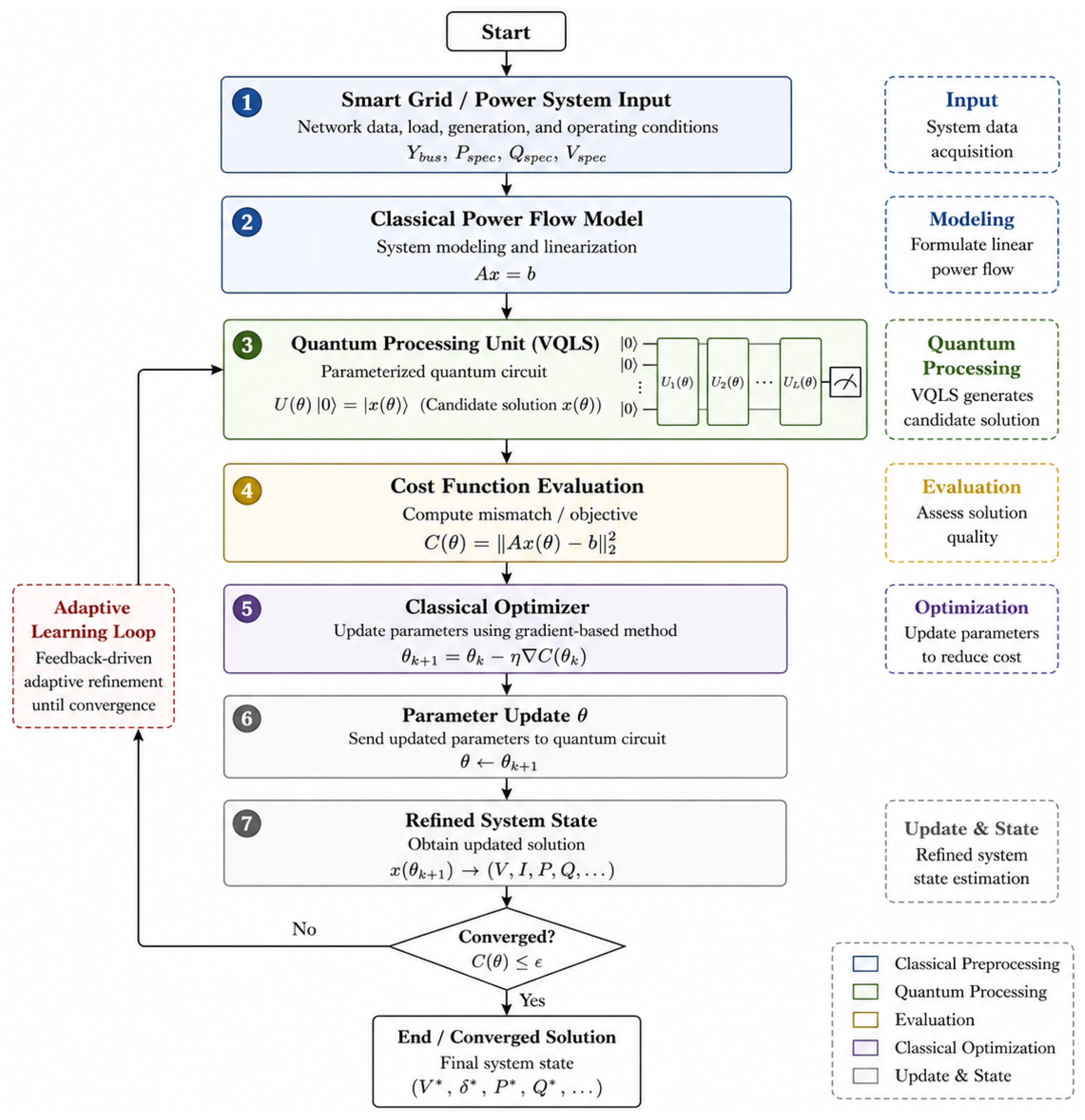
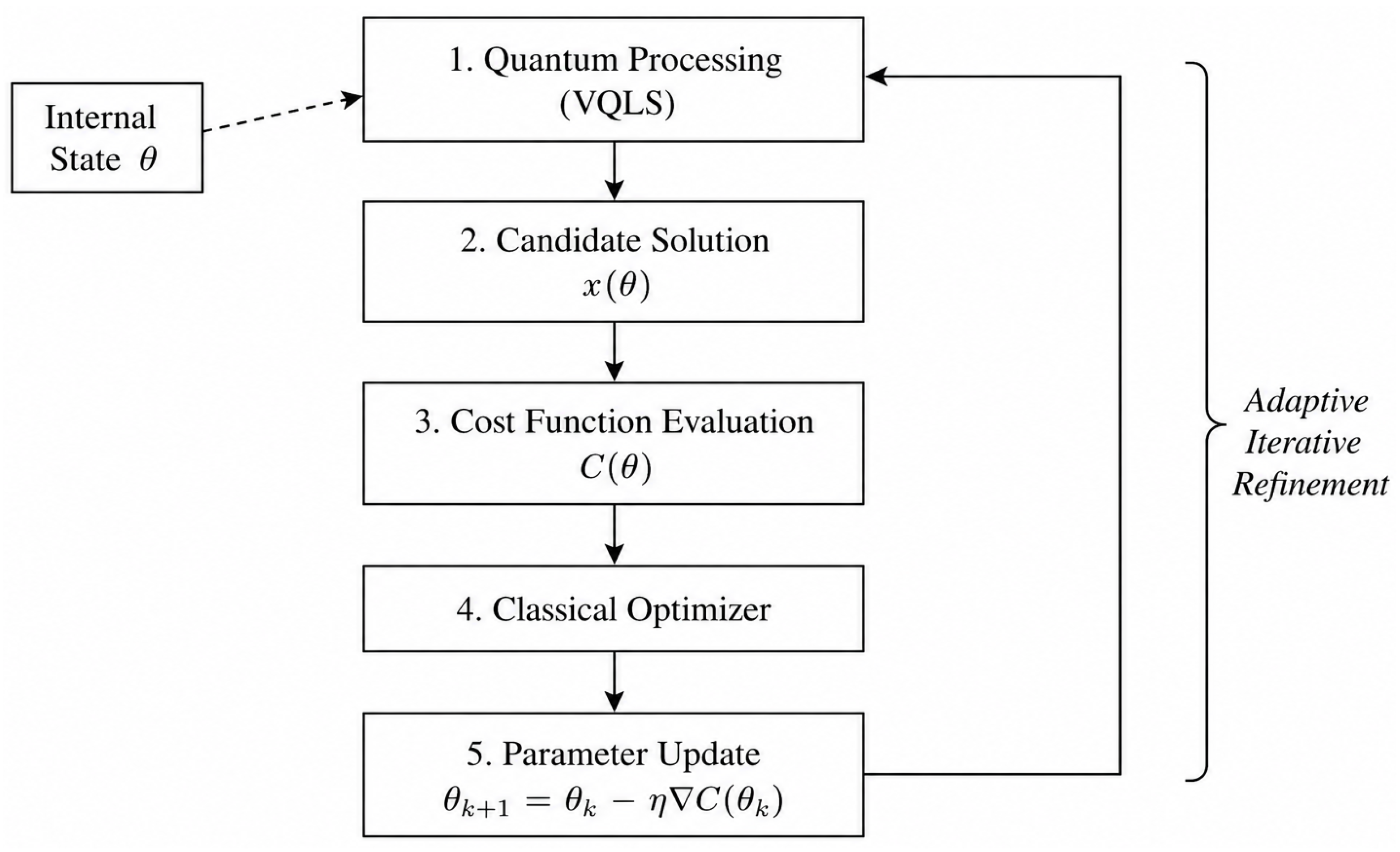
Figure 1 illustrates the overall structure of the proposed framework. The VQLS is used as an approximate linear-system solver within the conventional iterative AC power flow process rather than as a replacement for classical network modeling.

2.2. Power Flow Problem Formulation

Power flow analysis determines the steady-state voltage magnitude and phase angle at each bus for specified generation, load demand, and network parameters. In this study, the electrical network is represented using the conventional nodal admittance formulation employed in Newton–Raphson power flow analysis [13,17].

The relationship between the injected bus-current vector and the complex bus-voltage vector is expressed as

$$\mathbf{I}={\mathbf{Y}}_{\mathrm{bus}}\mathbf{V},$$

(1)

where $\mathbf{I}\in {\mathbb{C}}^n$ is the injected-current vector, $\mathbf{V}\in {\mathbb{C}}^n$ is the complex bus-voltage vector, ${\mathbf{Y}}_{\mathrm{bus}}\in {\mathbb{C}}^{n\times n}$ is the bus admittance matrix, and n is the number of buses.

The complex voltage at bus i is written as

$$V_i=|V_i|e^{j{\delta }_i},$$

(2)

where $|V_i|$ and ${\delta }_i$ denote the voltage magnitude and phase angle, respectively. The complex power injected at bus i is

$$S_i=P_i+j{Q}_i=V_i{I}_i^{\ast },$$

(3)

where $P_i$ and $Q_i$ are the active- and reactive-power injections, and the superscript ∗ denotes complex conjugation.

Using $Y_{ij}=G_{ij}+j{B}_{ij}$, the active- and reactive-power injections are given by

$$P_i={\displaystyle \sum _{j=1}^n}|V_i||V_j|\left[G_{ij}\cos ({\delta }_i-{\delta }_j)+B_{ij}\sin ({\delta }_i-{\delta }_j)\right],$$

(4)

and

$$Q_i={\displaystyle \sum _{j=1}^n}|V_i||V_j|\left[G_{ij}\sin ({\delta }_i-{\delta }_j)-B_{ij}\cos ({\delta }_i-{\delta }_j)\right].$$

(5)

Because Equations (4) and (5) are nonlinear, the Newton–Raphson method solves them through successive linearization [13,14]. At power flow iteration k, the active- and reactive-power mismatches are defined as

$$\Delta P_i^{\left(k\right)}=P_{i,\mathrm{spec}}-P_i^{\left(k\right)},$$

(6)

and

$$\Delta Q_i^{\left(k\right)}=Q_{i,\mathrm{spec}}-Q_i^{\left(k\right)},$$

(7)

where the subscript “spec” denotes the specified bus injection, and the superscript $\left(k\right)$ denotes the calculated value at the current iteration.

The mismatch vector and state-correction vector are related through the Jacobian matrix as

$$\left[\begin{array}{c}\Delta {\mathbf{P}}^{\left(k\right)}\\ \Delta {\mathbf{Q}}^{\left(k\right)}\end{array}\right]={\left[\begin{array}{cc}{\mathbf{J}}_{P\delta }& {\mathbf{J}}_{PV}\\ {\mathbf{J}}_{Q\delta }& {\mathbf{J}}_{QV}\end{array}\right]}^{\left(k\right)}\left[\begin{array}{c}\Delta {\mathit{\delta }}^{\left(k\right)}\\ \Delta {\mathbf{V}}^{\left(k\right)}\end{array}\right].$$

(8)

For integration with the VQLS, Equation (8) is written in the compact form

$${\mathbf{A}}^{\left(k\right)}{\mathbf{x}}^{\left(k\right)}={\mathbf{b}}^{\left(k\right)},$$

(9)

where

$${\mathbf{A}}^{\left(k\right)}={\mathbf{J}}^{\left(k\right)},{\mathbf{x}}^{\left(k\right)}=\left[\begin{array}{c}\Delta {\mathit{\delta }}^{\left(k\right)}\\ \Delta {\mathbf{V}}^{\left(k\right)}\end{array}\right],{\mathbf{b}}^{\left(k\right)}=\left[\begin{array}{c}\Delta {\mathbf{P}}^{\left(k\right)}\\ \Delta {\mathbf{Q}}^{\left(k\right)}\end{array}\right].$$

(10)

Reduced-System Construction and Full-State Reconstruction

The complete Newton–Raphson correction vector contains the voltage-angle and voltage-magnitude corrections associated with the non-slack buses. For the IEEE 33-bus test system, this full correction vector is larger than the dimension that can be represented by the four-qubit VQLS circuit used in this proof-of-concept study. Therefore, the full Jacobian equation was partitioned into a quantum block containing 16 selected state variables and a complementary block containing the remaining variables.

The 16-dimensional quantum block was selected as a fixed subset of the complete correction vector before the VQLS optimization was performed. The same variable indices were maintained throughout all power flow iterations to preserve a consistent mapping between the reduced quantum system and the full classical state vector. This selection was used to make the problem dimension compatible with the four-qubit state representation and should not be interpreted as an optimized or universally best variable-selection strategy.

The partitioned linear system was written as

$$\left[\begin{array}{cc}{\mathbf{J}}_{qq}& {\mathbf{J}}_{qc}\\ {\mathbf{J}}_{cq}& {\mathbf{J}}_{cc}\end{array}\right]\left[\begin{array}{c}\Delta {\mathbf{z}}_q\\ \Delta {\mathbf{z}}_c\end{array}\right]=\left[\begin{array}{c}\Delta {\mathbf{s}}_q\\ \Delta {\mathbf{s}}_c\end{array}\right],$$

(11)

where $\Delta {\mathbf{z}}_q\in {\mathbb{R}}^{16}$ denotes the selected state-correction variables represented by the VQLS module, $\Delta {\mathbf{z}}_c$ denotes the remaining correction variables, $\Delta {\mathbf{s}}_q$ and $\Delta {\mathbf{s}}_c$ are the corresponding mismatch-vector partitions, and ${\mathbf{J}}_{qq}$, ${\mathbf{J}}_{qc}$, ${\mathbf{J}}_{cq}$, and ${\mathbf{J}}_{cc}$ are the associated Jacobian submatrices.

The reduced 16 × 16 system was obtained using the Schur complement as

$${\mathbf{A}}_{\mathrm{red}}={\mathbf{J}}_{qq}-{\mathbf{J}}_{qc}{\mathbf{J}}_{cc}^{-1}{\mathbf{J}}_{cq},$$

(12)

and

$${\mathbf{b}}_{\mathrm{red}}=\Delta {\mathbf{s}}_q-{\mathbf{J}}_{qc}{\mathbf{J}}_{cc}^{-1}\Delta {\mathbf{s}}_c.$$

(13)

The VQLS was then used to approximate

$${\mathbf{A}}_{\mathrm{red}}\Delta {\mathbf{z}}_q={\mathbf{b}}_{\mathrm{red}}.$$

(14)

After reconstructing the 16-dimensional quantum solution, the correction vector for the complementary variables was recovered by classical back-substitution:

$$\Delta {\mathbf{z}}_c={\mathbf{J}}_{cc}^{-1}\left(\Delta {\mathbf{s}}_c-{\mathbf{J}}_{cq}\Delta {\mathbf{z}}_q\right).$$

(15)

Finally, $\Delta {\mathbf{z}}_q$ and $\Delta {\mathbf{z}}_c$ were returned to their original positions in the complete state-correction vector. The reconstructed full correction vector was subsequently used in the classical power flow iteration to update the voltage angles and voltage magnitudes of the 33-bus system.

The computational overhead of this reduction consists of the partitioning of the full Jacobian, construction of the Schur complement, solution or factorization associated with ${\mathbf{J}}_{cc}$, and classical back-substitution. These operations are not included in the VQLS circuit-depth index reported in the resource-scaling assessment. The circuit-depth index therefore reflects only the variational circuit representation and should not be interpreted as the total computational cost of the hybrid method.

Because the reduced system depends on the selected state variables and on the conditioning of the Jacobian submatrices, the accuracy of the final voltage profile may vary with the selected quantum-variable set. In this study, the fixed 16-variable selection was used for numerical consistency in the proof-of-concept evaluation. A systematic comparison of alternative variable-selection strategies is left for future work.

2.3. Variational Quantum Linear Solver

The VQLS reformulates the solution of a linear system as a variational optimization problem [27]. Instead of explicitly forming ${\mathbf{A}}^{-1}$, the method prepares a parameterized trial state and adjusts its parameters to reduce the residual between the candidate solution and the target linear system.

For each linearized power flow equation, the right-hand-side vector is normalized as

$$|b\rangle ={\displaystyle \frac{\mathbf{b}}{{\parallel \mathbf{b}\parallel }_2}}.$$

(16)

The approximate solution is represented by the parameterized quantum state

$$|x\left(\mathit{\theta }\right)\rangle ={U\left(\mathit{\theta }\right)|0\rangle }^{\otimes n_q},$$

(17)

where $U\left(\mathit{\theta }\right)$ is the parameterized circuit, $\mathit{\theta }$ is the trainable parameter vector, and $n_q$ is the number of qubits used in the simulation.

The candidate solution is evaluated using the residual-based cost function

$$C\left(\mathit{\theta }\right)={∥\mathbf{A}\mathbf{x}\left(\mathit{\theta }\right)-\mathbf{b}∥}_2^2,$$

(18)

where $\mathbf{x}\left(\mathit{\theta }\right)$ denotes the classical vector reconstructed from the trial state. A reduction in $C\left(\mathit{\theta }\right)$ indicates closer agreement between the candidate vector and the Jacobian-based linear equation.

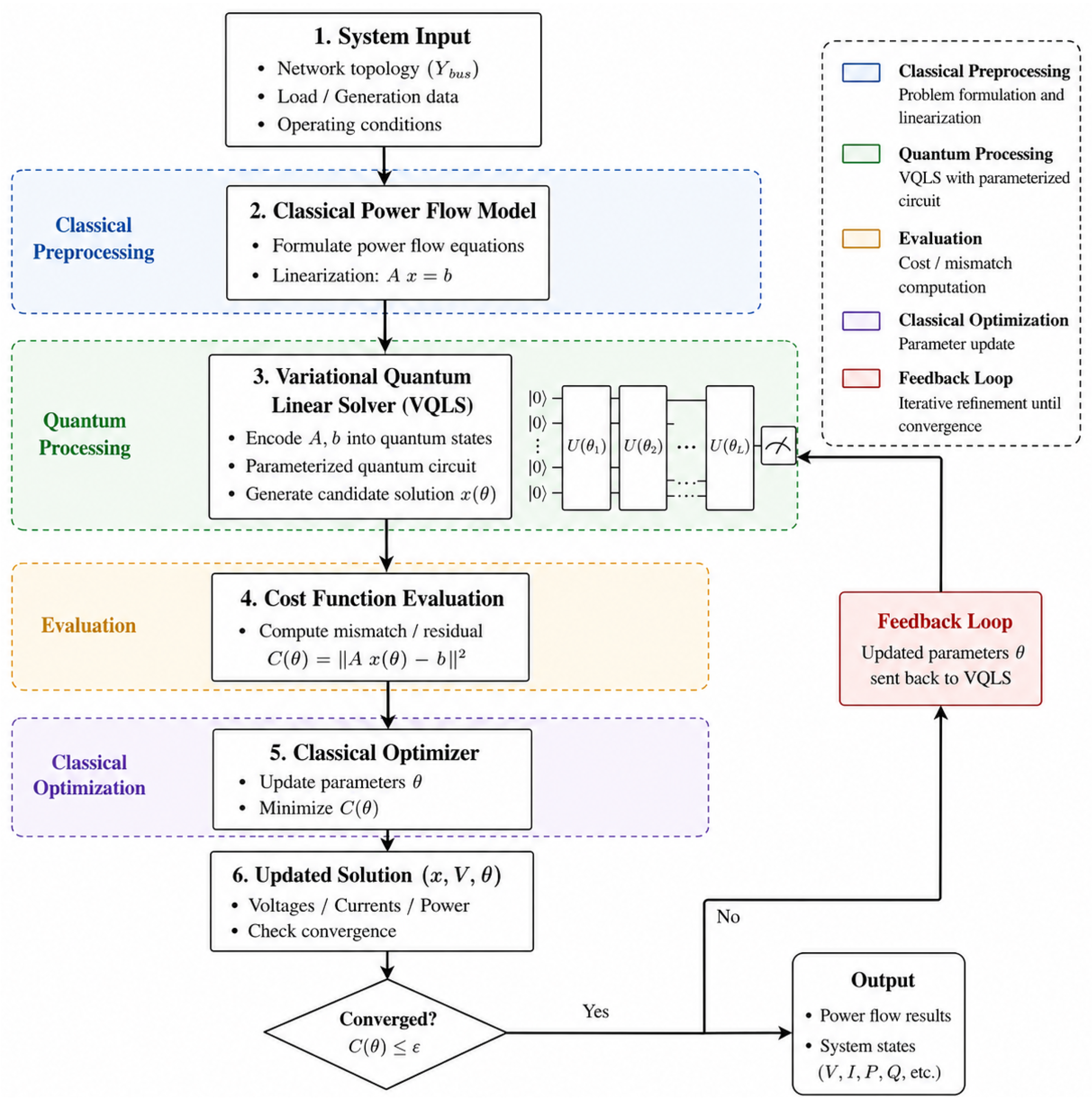
Figure 2 summarizes the computational sequence. The classical stage constructs $\mathbf{A}$ and $\mathbf{b}$, the variational circuit generates a candidate state, and the residual cost is evaluated and returned to the classical optimizer.

At the end of the inner optimization process, the approximate state-correction vector is reconstructed and returned to the classical power flow model. The reconstructed correction vector is subsequently used to update the voltage magnitudes and phase angles within the classical power flow iteration.

The present implementation is intended to investigate the numerical feasibility of integrating VQLS with AC power flow analysis. It does not claim a demonstrated quantum computational advantage because quantum state preparation, finite-shot measurement, hardware noise, circuit-execution overhead, and execution time on physical quantum hardware were not included in the present evaluation [24,26,27].

2.4. Classical Optimization Using COBYLA

The circuit parameters were optimized using the Constrained Optimization by Linear Approximation (COBYLA) algorithm. COBYLA is a derivative-free trust-region method that constructs local linear approximations of the objective function and constraints [28]. Its derivative-free structure is suitable for variational quantum calculations because it avoids the direct evaluation of analytical gradients.

At optimization iteration t, the circuit produces a candidate solution $\mathbf{x}\left({\mathit{\theta }}_t\right)$, and its cost is evaluated as

$$C_t={∥\mathbf{A}\mathbf{x}\left({\mathit{\theta }}_t\right)-\mathbf{b}∥}_2^2.$$

(19)

The optimization objective is

$${\mathit{\theta }}^{\ast }=\underset{\mathit{\theta }}{\arg \min }C\left(\mathit{\theta }\right),$$

(20)

where ${\mathit{\theta }}^{\ast }$ is the parameter vector associated with the lowest cost identified during the optimization process.

Figure 3 illustrates the iterative exchange among the parameterized circuit, cost-function evaluation, and COBYLA optimizer. The parameter update is performed internally by COBYLA and is not expressed as a gradient-descent equation.

The optimization terminates when the change in cost becomes smaller than the selected stability tolerance or when the maximum number of COBYLA iterations is reached. Because the reported cost trajectory approaches a small but nonzero stationary value, convergence in this study refers to stabilization of the optimization process rather than exact elimination of the residual.

2.5. Modified IEEE 33-Bus Distribution System with V2G Integration

The proposed method was evaluated using the IEEE 33-bus radial distribution system introduced by Baran and Wu [19]. The network consists of a main radial feeder and several lateral branches. Bus 1 was treated as the slack bus, while the remaining buses were represented as load buses with specified active- and reactive-power demands.

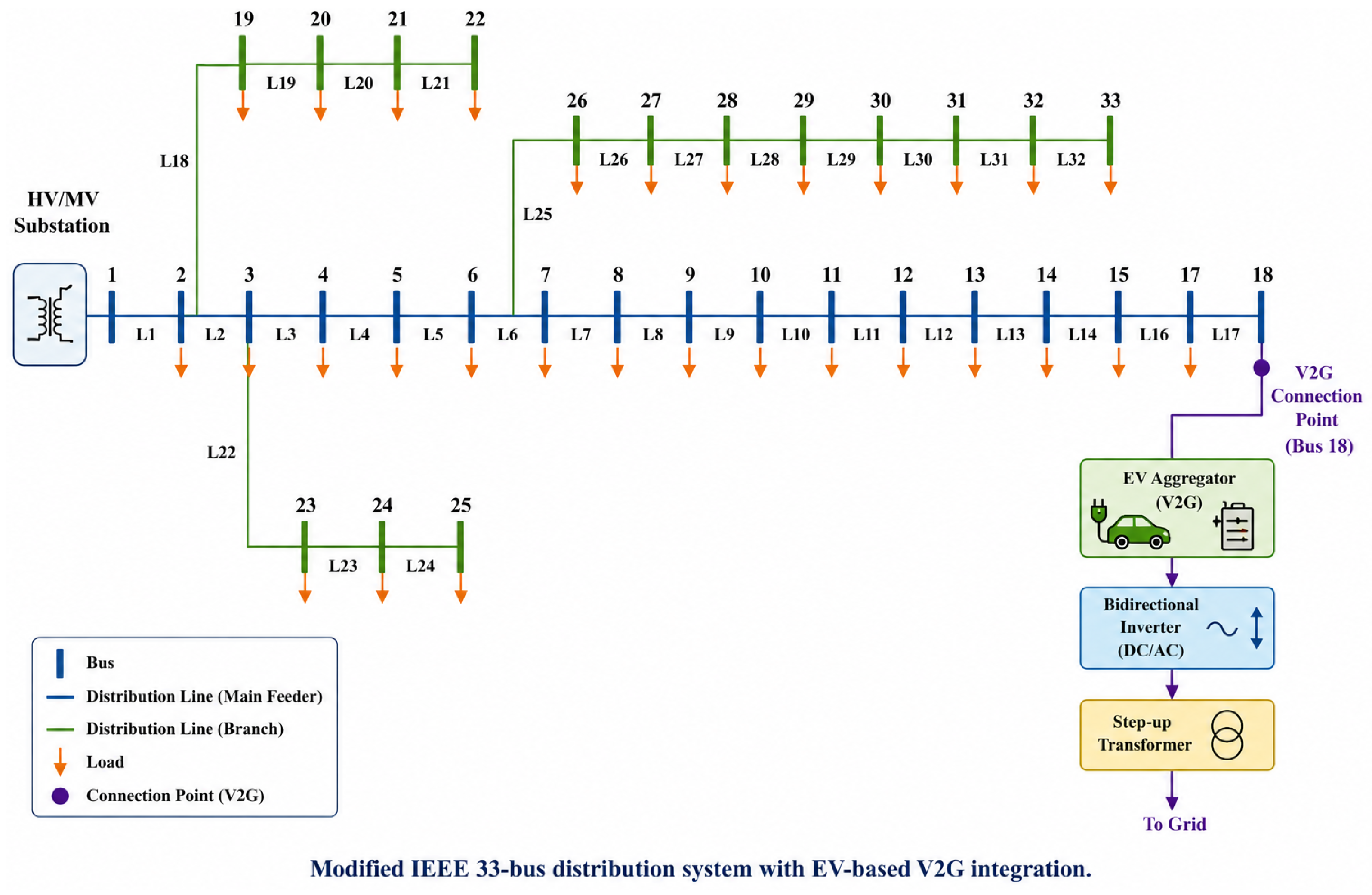
The network was modified by connecting an aggregated EV-based V2G unit at Bus 18. In the steady-state model, the V2G unit was represented through its net active- and reactive-power exchange with the distribution network. This representation follows the fundamental V2G concept in which connected EV batteries can operate as controllable loads during charging and as distributed energy resources during discharging [2].

The net active- and reactive-power injections at Bus 18 were represented as

$$P_{18}^{\mathrm{net}}=P_{18}^{\mathrm{V}2\mathrm{G}}-P_{18}^{\mathrm{L}},$$

(21)

and

$$Q_{18}^{\mathrm{net}}=Q_{18}^{\mathrm{V}2\mathrm{G}}-Q_{18}^{\mathrm{L}},$$

(22)

where $P_{18}^{\mathrm{L}}$ and $Q_{18}^{\mathrm{L}}$ are the local load demands, while $P_{18}^{\mathrm{V}2\mathrm{G}}$ and $Q_{18}^{\mathrm{V}2\mathrm{G}}$ denote the specified V2G power exchange. A positive $P_{18}^{\mathrm{V}2\mathrm{G}}$ denotes power injection into the feeder, whereas a negative value denotes charging demand.

The V2G interface was modeled only at the steady-state power flow level. Converter switching, battery electrochemical dynamics, state-of-charge scheduling, communication delays, and electricity-market operation were outside the scope of this study. Figure 4 shows the modified IEEE 33-bus network and the location of the V2G unit.

The same network topology, line parameters, bus loads, slack-bus condition, initial voltage profile, and V2G operating point were used for both the proposed method and the Newton–Raphson reference method.

2.6. V2G Participation and Active Power Loss Assessment

The daily active- and reactive-power demands were represented by applying a time-dependent loading factor to the original IEEE 33-bus data:

$$P_i^{\mathrm{L}}\left(t\right)=\lambda \left(t\right)P_{i,0}^{\mathrm{L}},Q_i^{\mathrm{L}}\left(t\right)=\lambda \left(t\right)Q_{i,0}^{\mathrm{L}},$$

(23)

where $P_{i,0}^{\mathrm{L}}$ and $Q_{i,0}^{\mathrm{L}}$ are the original active- and reactive-power demands at bus i, respectively, and $\lambda \left(t\right)$ is the normalized 24-h loading profile.

For scenario s, the active power supplied by the aggregated V2G resource at Bus 18 was defined as

$$P_{18,\mathrm{V}2\mathrm{G}}^{\left(s\right)}\left(t\right)={\rho }_s{P}_{\mathrm{agg}}^{\mathrm{rated}}u\left(t\right),$$

(24)

where ${\rho }_s$ is the V2G participation ratio, $P_{\mathrm{agg}}^{\mathrm{rated}}$ is the rated active-power capacity of the complete EV aggregation, and $u\left(t\right)$ is the prescribed normalized discharge profile. The participation ratios were defined as

$${\rho }_s\in \left\{0,0.20,0.50\right\},$$

(25)

corresponding to the base case without V2G support, the 20% V2G participation case, and the 50% V2G participation case, respectively. The discharge profile was set to zero outside the selected V2G-support period. In addition to the three prescribed V2G participation cases, additional stress-test operating scenarios were considered to examine the loss-reduction behavior under more severe network conditions. These scenarios included an N-1 contingency case, an N-1 contingency case with V2G emergency support, and a dynamic railway-peak loading case with V2G support. These cases were used as prescribed operating conditions for numerical assessment and should not be interpreted as a full security-constrained optimization, complete railway-load optimization, or market-based V2G dispatch framework. At each time step, the total active power loss was calculated as

$$P_{\mathrm{loss}}\left(t\right)={\displaystyle \sum _{\ell =1}^{N_{\mathrm{line}}}}{R}_{\ell }{\left|I_{\ell }\left(t\right)\right|}^2,$$

(26)

where $R_{\ell }$ is the resistance of line ℓ, $I_{\ell }\left(t\right)$ is the corresponding line current at time t, and $N_{\mathrm{line}}$ is the total number of distribution lines. The operating conditions used in the scenario analysis are summarized in

Table 2. Parameters and operating conditions used in the V2G scenario assessment.

Parameter	Value or Description
Test system	Modified IEEE 33-bus radial distribution system
V2G connection bus	Bus 18
Assessment horizon	24 h
Base-case participation ratio	0% (no V2G support)
Moderate V2G participation ratio	20% of the aggregated EV resource
High V2G participation ratio	50% of the aggregated EV resource
V2G support period	Evening high-demand period, approximately 15:00–23:00
V2G operating profile	Prescribed active-power discharge profile during the high-demand period
Reactive-power treatment	Reactive-power support was not varied among the V2G scenarios; the scenario comparison focused on active-power injection and active power losses.
Load representation	The same normalized 24-h loading profile was applied to the original IEEE 33-bus load data for the principal V2G participation cases. Additional prescribed loading was applied only for the specified stress-test case.
Network conditions	The same feeder topology, line parameters, and bus-load distribution were maintained for the principal V2G participation cases. For the additional stress-test cases, the specified contingency or dynamic loading condition was applied.
Active power loss calculation	Equation (26)

.

At each time step, the power flow was solved using the specified feeder topology, line parameters, bus-load distribution, normalized loading profile, and V2G support condition. For the principal V2G participation cases, only the V2G participation ratio and the associated active-power injection were changed. For the additional stress-test cases, the specified contingency or dynamic loading condition was also applied. Therefore, the differences in the calculated active power losses were associated with the prescribed V2G support and the corresponding operating condition.

2.7. Additional Convergence and Resource-Scaling Assessments

2.7.1. Relationship Between the Two Convergence Runs

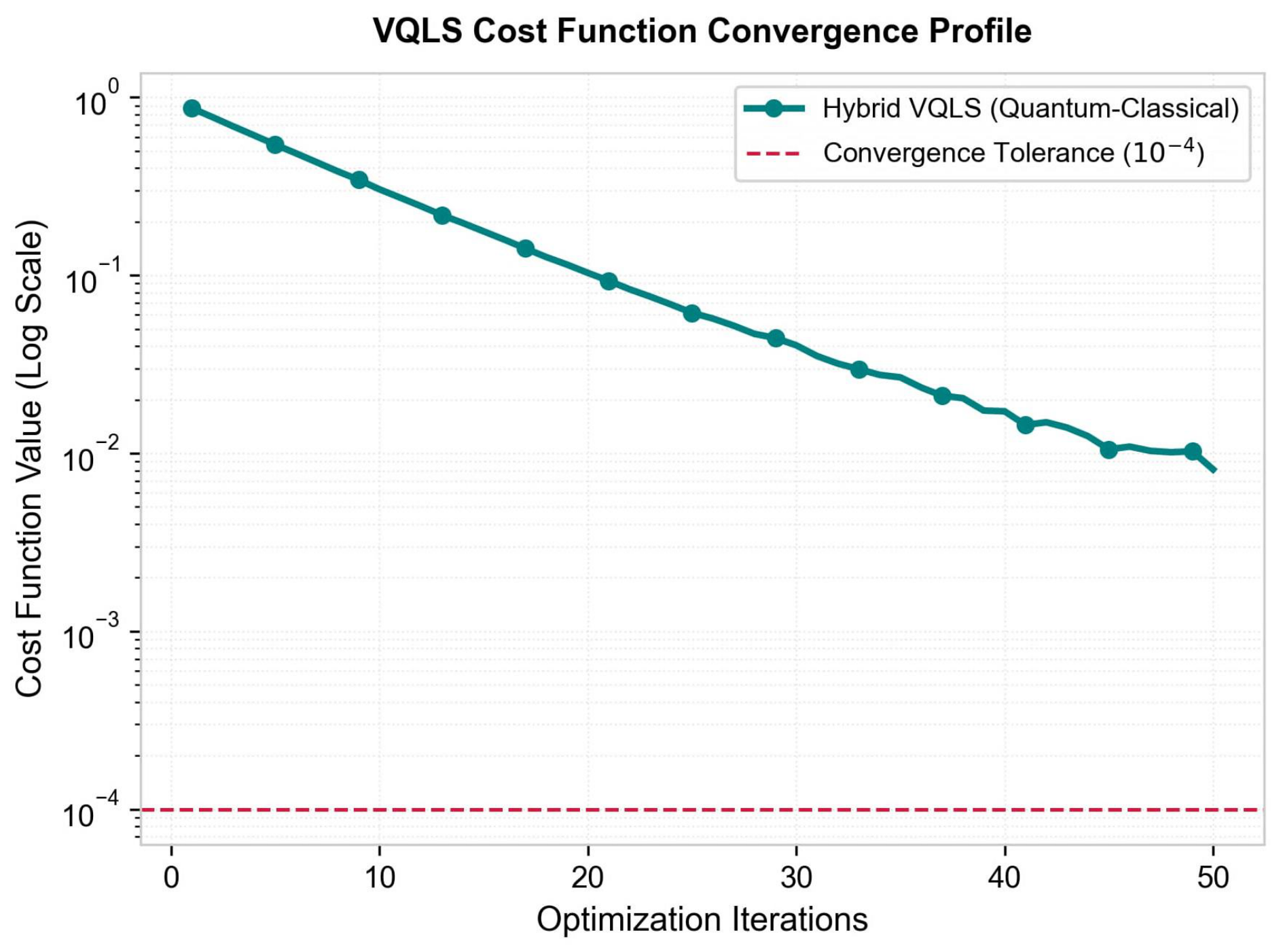
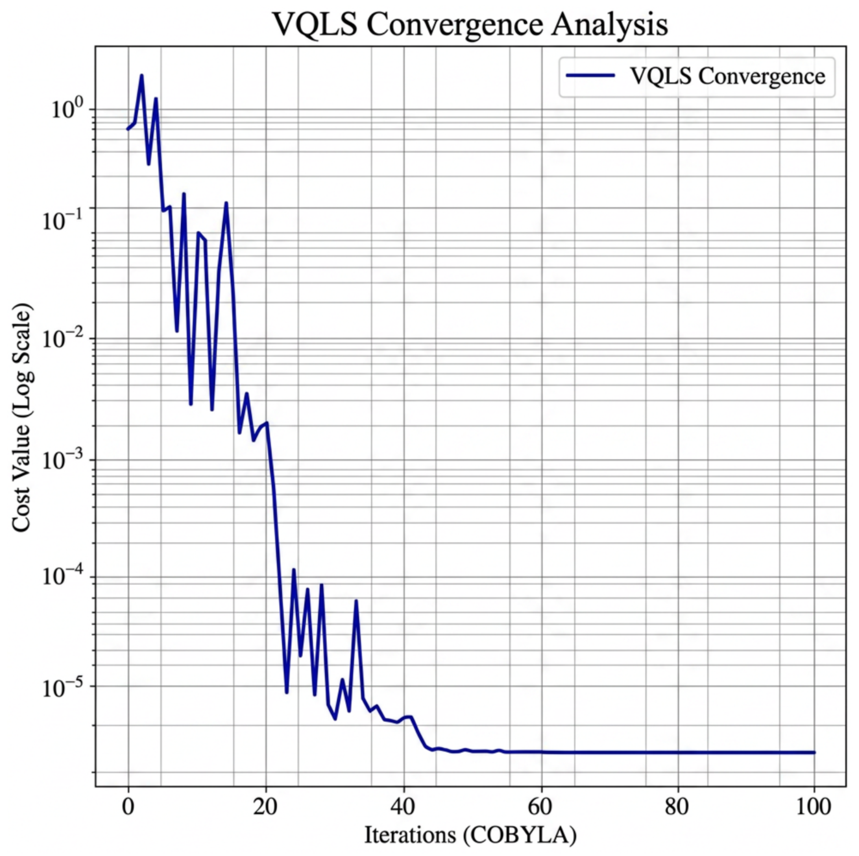
Two separate VQLS–COBYLA runs were conducted for different purposes. The main run shown in Figure 5 was used to obtain the approximate state-correction vector employed in the IEEE 33-bus voltage-profile calculation. The optimization was evaluated using a maximum budget of 100 COBYLA iterations.

The additional run was performed independently to examine the cost reduction within a fixed iteration budget. It used the same reduced matrix, right-hand-side vector, Real-Amplitudes ansatz, and COBYLA configuration as the main run. However, the variational parameters were initialized independently, and the optimization was limited to 50 iterations. The value of ${10}^{-4}$ was used as a reference accuracy threshold rather than as a guaranteed stopping criterion. The principal settings of the two convergence runs are summarized in

Table 3. Settings used in the main and additional VQLS–COBYLA convergence runs.

Setting	Main Run	Additional Run
Purpose	Generation of the approximate correction vector used in the voltage-profile calculation	Independent fixed-budget convergence assessment
Maximum COBYLA iterations	100	50
Convergence interpretation	Stabilization of the cost function within the available iteration budget	Cost reduction relative to the reference threshold of ${10}^{-4}$
Parameter initialization	Initial parameter vector used for the primary optimization run	Independently initialized parameter vector
Reduced linear system	${\mathbf{A}}_{\mathrm{red}}\Delta {\mathbf{z}}_q={\mathbf{b}}_{\mathrm{red}}$	Same reduced linear system
Circuit ansatz	Real-Amplitudes with three repetitions	Real-Amplitudes with three repetitions
Classical optimizer	COBYLA	COBYLA

.

Because the two runs used independently initialized parameter vectors and different iteration budgets, their cost trajectories were not expected to coincide. The main run supported the reported power flow calculation, whereas the additional run was used to examine whether the optimization could approach a stricter reference threshold within a limited number of iterations. The additional run reduced the cost substantially but did not reach the prescribed value of ${10}^{-4}$ within 50 iterations.

2.7.2. Classical and VQLS Resource-Scaling Metrics

A preliminary resource-scaling assessment was conducted for systems containing 14, 33, 70, 118, and 300 buses. The purpose of this assessment was to compare the growth trends of two normalized resource indicators rather than to provide a direct execution-time comparison.

For a system containing $N_b$ buses, a uniform state-dimension proxy was defined as

$$m_{\mathrm{p}}\left(N_b\right)=2(N_b-1),$$

(27)

where $m_{\mathrm{p}}$ represents the approximate number of voltage-angle and voltage-magnitude variables when all non-slack buses are treated uniformly. This expression was used only to provide a consistent dimensional reference across the examined system sizes.

The corresponding quantum encoding size was estimated as

$$n_q\left(N_b\right)=⌈{\log }_2{m}_{\mathrm{p}}\left(N_b\right)⌉.$$

(28)

For the classical solver, the plotted computation index was defined as

$$I_{\mathrm{C}}\left(N_b\right)={\displaystyle \frac{N_b^2}{20}}.$$

(29)

The factor of 20 was used to normalize the index to a convenient plotting range. Therefore, $I_{\mathrm{C}}$ is a dimensionless computation index and should not be interpreted as the exact number of floating-point operations required by an LU or Newton–Raphson implementation.

The VQLS circuit-depth trend was represented by an empirical logarithmic relation fitted to the circuit-depth values used in the scaling assessment:

$$D_{\mathrm{VQLS}}\left(N_b\right)=3.261+17.676\ln \left(N_b\right),$$

(30)

where $D_{\mathrm{VQLS}}$ is the circuit-depth index and $\ln (·)$ denotes the natural logarithm. The calculated values were rounded to the nearest integer for presentation in the resourcescaling analysis. The numerical values used to generate the resource-scaling result are summarized in

Table 4. Numerical values used to generate the computational resource-scaling result.

Bus Size	State-Dimension Proxy, ${\mathit{m}}_{\mathbf{p}}$	Qubits, ${\mathit{n}}_{\mathit{q}}$	Classical Computation Index, ${\mathit{I}}_{\mathbf{C}}$	VQLS Circuit-Depth Index, ${\mathit{D}}_{\mathbf{VQLS}}$
14	26	5	9.80	50
33	64	6	54.45	65
70	138	8	245.00	78
118	234	8	696.20	88
300	598	10	4500.00	104

.

The two indicators have different meanings and are displayed using separate vertical axes. The classical index reflects a normalized growth model based on system size, whereas the VQLS index represents the fitted circuit-depth trend. The comparison therefore illustrates relative scaling behavior only. It does not establish equivalent computational cost, execution-time advantage, or quantum speedup.

2.8. Reference Method and Performance Evaluation

The conventional Newton–Raphson method was used as the numerical reference because it is an established approach for solving nonlinear AC power flow equations [13,14]. For the IEEE 33-bus voltage comparison, both methods used the same network parameters, initial operating condition, specified bus injections, and V2G operating condition.

For the Newton–Raphson method, the state-correction vector was obtained by solving

$${\mathbf{J}}^{\left(k\right)}\Delta {\mathbf{z}}^{\left(k\right)}=\Delta {\mathbf{s}}^{\left(k\right)},$$

(31)

where ${\mathbf{J}}^{\left(k\right)}$ is the Jacobian matrix, $\Delta {\mathbf{z}}^{\left(k\right)}$ is the state-correction vector, and $\Delta {\mathbf{s}}^{\left(k\right)}$ is the power-mismatch vector.

For the proposed method, the corresponding reduced Jacobian subproblem was supplied to the VQLS, and the approximate correction vector was obtained through the VQLS–COBYLA optimization loop.

The numerical evaluation considered the following outputs:

• the evolution and stabilization of the main VQLS cost trajectory during the 100-iteration COBYLA optimization;
• the cost reduction relative to the reference tolerance of 10⁻⁴ during the additional 50-iteration assessment;
• the agreement between the bus-voltage magnitude profiles obtained using the proposed method and the Newton–Raphson reference method;
• the variation in active power losses under the base, 20% V2G, and 50% V2G participation scenarios over the 24-h assessment period; and
• the respective growth trends of the normalized classical computation index and the VQLS circuit-depth index as the system size increased.

The bus-wise absolute voltage deviation was defined as

$$e_i=\left|V_i^{\mathrm{VQLS}}-V_i^{\mathrm{NR}}\right|,$$

(32)

where $V_i^{\mathrm{VQLS}}$ and $V_i^{\mathrm{NR}}$ are the voltage magnitudes obtained using the proposed and reference methods, respectively.

The voltage comparison was based on the corresponding voltage-profile assessment. The active power loss assessment was based on the three V2G operating scenarios, while the scaling assessment compared the respective trends of the two resource indicators.

The evaluation was intended to examine numerical consistency, convergence behavior, V2G-related network effects, and preliminary resource-scaling patterns. Since the normalized classical computation index and VQLS circuit-depth index represent different resources, the present study does not provide a direct execution-time comparison or evidence of quantum computational speedup. Hardware noise, finite-shot effects, and physical quantum-hardware execution were also not included.

2.9. Accuracy, Conditioning, and Reproducibility Metrics

To move beyond visual comparison of voltage profiles, quantitative accuracy metrics were used to compare the proposed VQLS-based result with the Newton–Raphson reference solution. The bus-wise voltage-magnitude error was defined as

$$e_{V,i}=\left|V_i^{\mathrm{VQLS}}-V_i^{\mathrm{NR}}\right|,$$

(33)

where $V_i^{\mathrm{VQLS}}$ and $V_i^{\mathrm{NR}}$ are the voltage magnitudes obtained from the proposed method and the Newton–Raphson method, respectively. The mean absolute voltage error was calculated as

$${\mathrm{MAE}}_V={\displaystyle \frac{1}{N_b}}{\displaystyle \sum _{i=1}^{N_b}}\left|V_i^{\mathrm{VQLS}}-V_i^{\mathrm{NR}}\right|,$$

(34)

and the voltage root-mean-square error was calculated as

$${\mathrm{RMSE}}_V=\sqrt{{\displaystyle \frac{1}{N_b}}\sum _{i=1}^{N_b}{\left(V_i^{\mathrm{VQLS}}-V_i^{\mathrm{NR}}\right)}^2}.$$

(35)

The maximum voltage-magnitude error was defined as

$$e_{V,\max }=\underset{i}{\max }\left|V_i^{\mathrm{VQLS}}-V_i^{\mathrm{NR}}\right|.$$

(36)

When voltage-angle results were available, the bus-wise phase-angle error was defined as

$$e_{\delta ,i}=\left|{\delta }_i^{\mathrm{VQLS}}-{\delta }_i^{\mathrm{NR}}\right|,$$

(37)

where ${\delta }_i^{\mathrm{VQLS}}$ and ${\delta }_i^{\mathrm{NR}}$ are the voltage angles obtained from the proposed and reference methods, respectively.

The residual norm of the reduced VQLS linear system was also evaluated to quantify how closely the variational solution satisfied the reduced Jacobian equation:

$$r_{\mathrm{red}}={∥{\mathbf{A}}_{\mathrm{red}}\Delta {\mathbf{z}}_q-{\mathbf{b}}_{\mathrm{red}}∥}_2.$$

(38)

In addition, the maximum power mismatch after the power flow update was defined as

$$\Delta S_{\max }=\underset{i}{\max }\left(\left|\Delta P_i\right|,\left|\Delta Q_i\right|\right).$$

(39)

To assess the numerical conditioning of the reduced Jacobian system, the two-norm condition number was calculated as

$$\kappa \left({\mathbf{A}}_{\mathrm{red}}\right)={∥{\mathbf{A}}_{\mathrm{red}}∥}_2{∥{\mathbf{A}}_{\mathrm{red}}^{-1}∥}_2.$$

(40)

A larger value of $\kappa \left({\mathbf{A}}_{\mathrm{red}}\right)$ indicates a more ill-conditioned reduced system, which may amplify numerical errors and make the VQLS cost more difficult to minimize.

2.10. Convergence Criteria and Repeated Optimization Runs

Two convergence levels were distinguished in this study. The outer AC power flow procedure refers to the iterative update of bus voltage magnitudes and angles, whereas the inner VQLS optimization refers to the COBYLA-based minimization of the reduced-system residual cost.

For the inner VQLS optimization, the main run was limited to 100 COBYLA iterations. Stabilization of the cost function was interpreted as the point at which the cost changed only slightly within the available iteration budget. The additional convergence assessment was limited to 50 iterations and used ${10}^{-4}$ as a reference accuracy threshold. This value was used only as a reference threshold and not as a guaranteed stopping value.

Because variational optimization may depend on parameter initialization, the sensitivity of the VQLS–COBYLA process was assessed using independent initial parameter vectors. The repeated-run analysis was used to summarize the mean, standard deviation, best value, and worst value of the final cost and accuracy metrics.

The final-cost statistics were calculated as

$${\overline{C}}_{\mathrm{final}}={\displaystyle \frac{1}{N_{\mathrm{run}}}}{\displaystyle \sum _{j=1}^{N_{\mathrm{run}}}}{C}_{\mathrm{final}}^{\left(j\right)},$$

(41)

and

$${\sigma }_C=\sqrt{{\displaystyle \frac{1}{N_{\mathrm{run}}-1}}\sum _{j=1}^{N_{\mathrm{run}}}{\left(C_{\mathrm{final}}^{\left(j\right)}-{\overline{C}}_{\mathrm{final}}\right)}^2},$$

(42)

where $N_{\mathrm{run}}$ is the number of independent optimization runs, and $C_{\mathrm{final}}^{\left(j\right)}$ is the final cost of run j.

2.11. Simulation Configuration and Resource Indicators

The numerical study was implemented in Python using Pandapower for the classical power flow calculations and Qiskit for the variational quantum simulation. The Qiskit Aer statevector simulator was used; therefore, finite-shot uncertainty, measurement error, limited device connectivity, and physical-hardware noise were not included.

For the detailed IEEE 33-bus proof-of-concept evaluation, a four-qubit Real-Amplitudes circuit was used to represent a normalized 16 × 16 reduced Jacobian subproblem. The circuit used three repetitions of the Real-Amplitudes ansatz. The ansatz configuration, optimizer setting, iteration budget, and reduced-system dimension are summarized in

Table 5. Simulation and evaluation settings used in the revised numerical study.

Parameter	Setting
Classical programming environment	Python
Power flow package	Pandapower
Quantum software framework	Qiskit
Quantum simulation backend	Qiskit Aer statevector simulator
Quantum solver	Variational Quantum Linear Solver (VQLS)
Parameterized circuit ansatz	Real-Amplitudes circuit
Real-Amplitudes repetitions	3
Number of qubits for the IEEE 33-bus proof of concept, $n_q$	4
Dimension of the reduced VQLS linear system	16 × 16
Matrix preparation	Partitioned full Jacobian with Schur-complement reduction and classical back-substitution
Classical optimizer	COBYLA
Main COBYLA iteration limit	100 iterations
Additional convergence assessment	50 iterations with a reference tolerance of ${10}^{-4}$
Power flow reference method	Newton–Raphson
Main test system	Modified IEEE 33-bus radial distribution system
V2G connection point	Bus 18
V2G operating scenarios	Base case without V2G support, 20% V2G participation, and 50% V2G participation
V2G assessment period	24 h
Classical resource indicator	Normalized classical computation index
VQLS resource indicator	VQLS circuit-depth index
Hardware-noise treatment	Not included; ideal statevector simulation was used
Finite-shot treatment	Not included; statevector expectation was used

.

The normalized classical computation index and the VQLS circuit-depth index were used only as separate resource indicators. They do not represent the same physical quantity and were not used to claim execution time advantage or quantum speedup. In addition, the VQLS circuit-depth index does not include state preparation, matrix encoding, repeated circuit evaluations, measurement shots, classical–quantum communication, optimizer overhead, Schur-complement construction, or full-state reconstruction.

The resource-scaling assessment used systems containing 14, 33, 70, 118, and 300 buses as representative distribution and transmission benchmark sizes. The assessment was intended to illustrate how the selected resource indicators change with system size, not to validate full VQLS power flow solutions for all examined systems.

3. Results

The proposed hybrid quantum–classical framework was evaluated using the modified IEEE 33-bus radial distribution system with the EV-based V2G unit connected at Bus 18. The numerical assessment considered the VQLS–COBYLA optimization behavior, quantitative agreement with the Newton–Raphson reference solution, conditioning of the reduced Jacobian subproblem, active power loss reduction under prescribed V2G support, repeated-run stability, and preliminary computational resource-scaling trends.

In this revised version, numerical summary tables are included to support the plotted results and to clarify the accuracy, conditioning, convergence, reproducibility, and resource-interpretation aspects of the proposed proof-of-concept implementation.

3.1. VQLS–COBYLA Optimization Behavior

Figure 5 shows the evolution of the VQLS cost function during the main COBYLA optimization run. At the beginning of the process, the cost exhibited relatively large variations while the optimizer explored the parameter space of the variational circuit. The overall cost subsequently decreased as improved candidate parameter sets were identified.

A marked reduction occurred during the early optimization stage. After the initial reduction period, the change in the cost became smaller and the curve approached a nearly stationary nonzero level. This behavior indicates that the VQLS–COBYLA process reached a stable region of the selected cost-function landscape under the implemented circuit and optimizer settings.

Table 6. Summary of the main VQLS–COBYLA optimization run under base and N-1 contingency cases.

Parameter/Metric	Base Case	N-1 Contingency
Problem dimension	16 × 16	16 × 16
Circuit ansatz	Real-Amplitudes	Real-Amplitudes
Number of parameters	16	16
Optimizer	COBYLA	COBYLA
Total iterations spent	80	80
Initial cost value	0.405533	0.203660
Final VQLS cost value, $C_{\mathrm{final}}$	0.081386	0.032900
Execution time (s)	0.45	0.42
Convergence interpretation	Cost reduction and stabilization within the prescribed iteration budget	Cost reduction and stabilization within the prescribed iteration budget

summarizes the numerical characteristics of the main VQLS–COBYLA run for the base and N-1 contingency cases. The reported result is interpreted as cost reduction and stabilization within the available iteration budget rather than exact convergence to a zero residual.

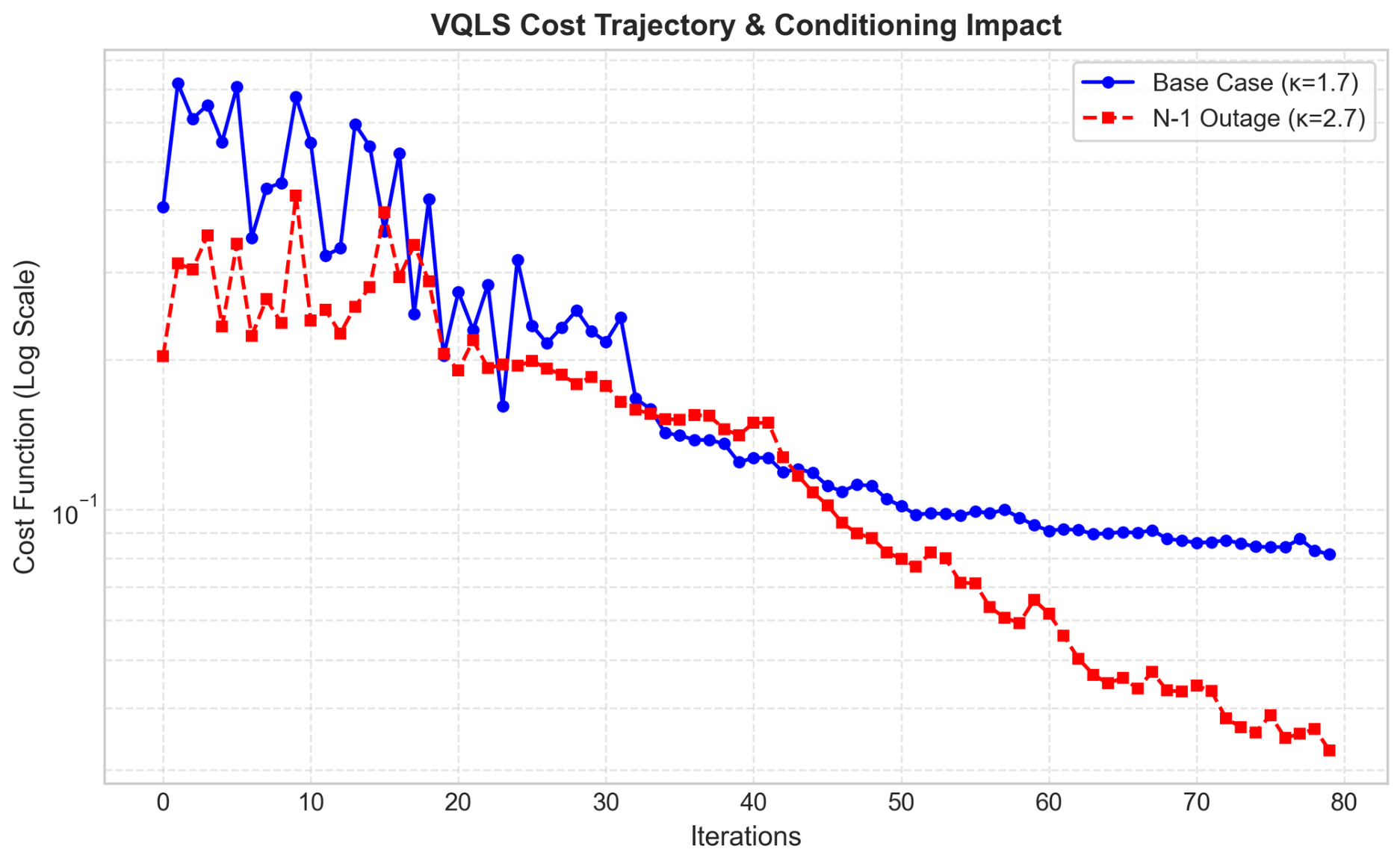
Figure 6 further compares the cost trajectories of the base and N-1 contingency cases. Although the N-1 contingency case had a higher reduced-system condition number, the optimizer still reduced the cost steadily within the 80-iteration budget. This result suggests that the examined contingency case increased the numerical sensitivity of the reduced system but did not prevent the VQLS–COBYLA loop from improving the candidate solution.

The base case reduced the VQLS cost from 0.405533 to 0.081386 within 80 COBYLA iterations, while the N-1 contingency case reduced the cost from 0.203660 to 0.032900. These results indicate that the VQLS–COBYLA loop was able to improve the candidate solution in both operating conditions. However, the nonzero final cost confirms that the result should be interpreted as an approximate variational solution rather than an exact solution of the reduced linear system.

3.2. Bus-Voltage Profile and Quantitative Accuracy Comparison

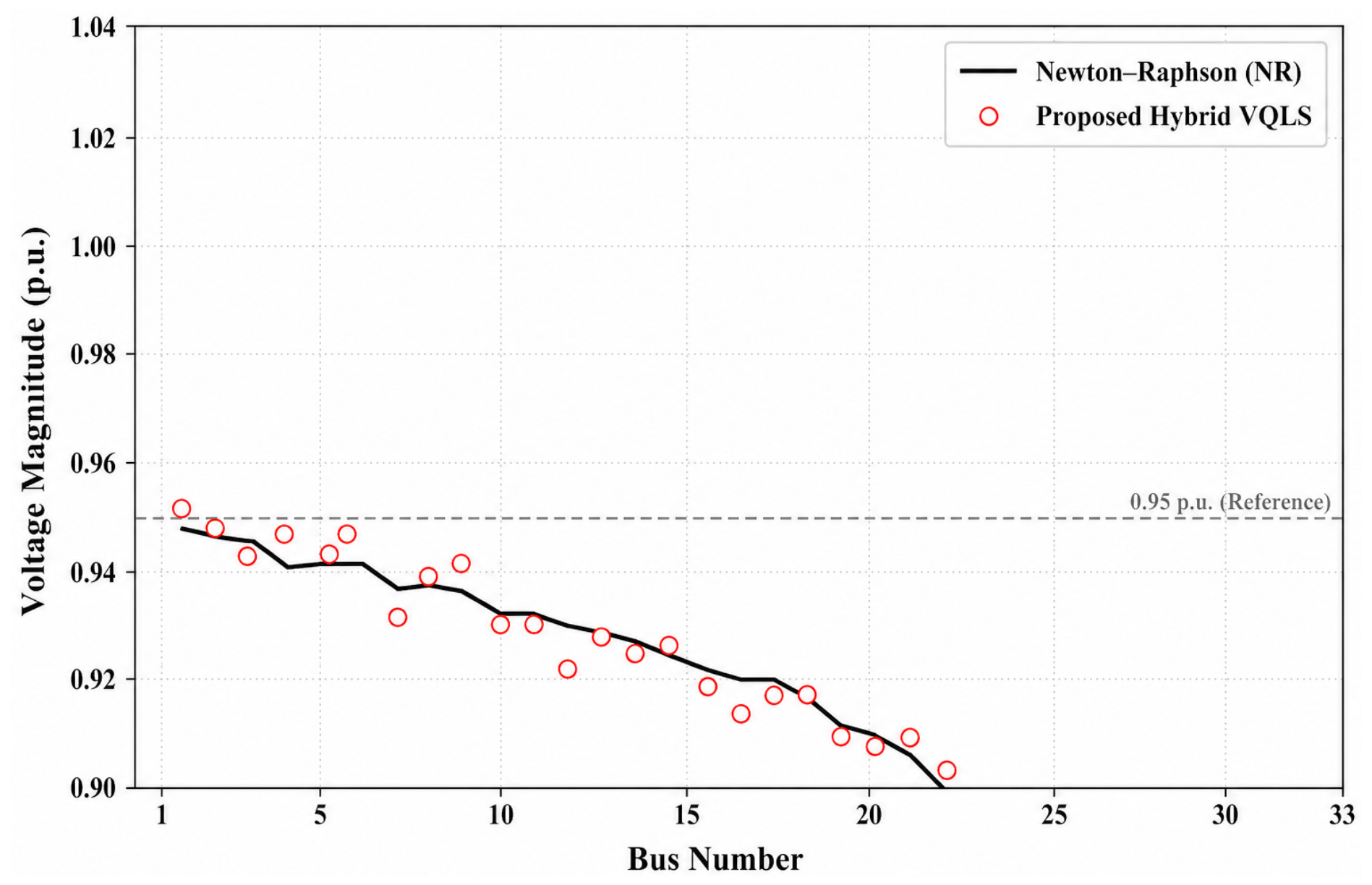
The state-correction vector obtained from the VQLS–COBYLA procedure was returned to the classical power flow model to update the voltage magnitudes and phase angles. Figure 7 compares the resulting voltage-magnitude profile with the reference solution obtained using the Newton–Raphson method.

Both methods produced the characteristic voltage pattern of a radial distribution feeder. The voltage magnitude was highest near the slack bus and generally decreased toward the downstream portion of the network because of the accumulated load demand and distribution-line impedances.

The voltage profile obtained using the proposed framework followed the overall trend of the Newton–Raphson solution. Small differences remained because the VQLS module produced an approximate reduced-system solution and the final cost did not reach zero. Therefore, the visual voltage-profile comparison was supported by additional quantitative metrics.

To provide a more rigorous comparison, quantitative error indices were calculated relative to the Newton–Raphson reference solution. The metrics include the mean absolute error, root-mean-square error, maximum absolute residual error, cosine similarity or fidelity, and relative error. The results are summarized in

Table 7. Quantitative accuracy metrics of the proposed VQLS-based solution relative to the Newton–Raphson reference solution.

Metric/Parameter	Base Case	N-1 Contingency
Mean absolute error (MAE)	$8.423265\times {10}^{-2}$	$6.441737\times {10}^{-2}$
Root mean square error (RMSE)	$1.007699\times {10}^{-1}$	$7.668041\times {10}^{-2}$
Maximum absolute residual error	$2.187494\times {10}^{-1}$	$1.774949\times {10}^{-1}$
Cosine similarity/fidelity, F	0.918763	0.952961
Relative error (%)	40.31	30.67

.

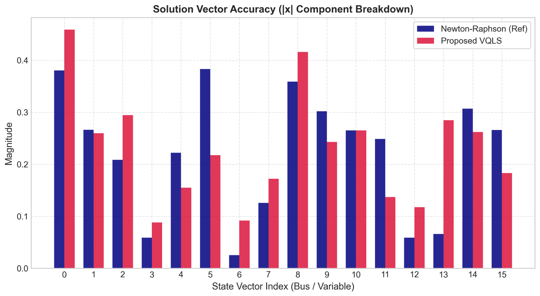
Figure 8 provides a component-wise view of the solution-vector accuracy. Several components of the VQLS-based solution closely follow the Newton–Raphson reference values, whereas larger deviations are visible for some state-vector components. These deviations explain the nonzero MAE, RMSE, and maximum absolute residual error reported in Table 7. The result confirms that the proposed method preserves the general reduced-system solution pattern but remains an approximate variational solution.

The N-1 contingency case produced lower MAE, RMSE, maximum absolute residual error, and relative error than the base case, while also producing a higher cosine similarity/fidelity value. This indicates that, for the examined reduced systems, the VQLS-based approximation was closer to the Newton–Raphson reference in the N-1 contingency case than in the base case. Nevertheless, the remaining relative error confirms that the proposed framework should be interpreted as an approximate reduced-system solver rather than an exact replacement for the Newton–Raphson method.

3.3. Conditioning of the Reduced Jacobian Subproblem

The condition number of the reduced Jacobian system was evaluated because matrix conditioning can affect both VQLS convergence and the accuracy of the reconstructed correction vector.

Table 8. Conditioning of the reduced Jacobian system used in the VQLS calculation.

Condition Metric	Base Case	N-1 Contingency
Matrix dimension	16 × 16	16 × 16
Maximum singular value, ${\sigma }_{\max }$	22.8144	21.9119
Minimum singular value, ${\sigma }_{\min }$	14.1340	8.2849
Two-norm condition number, ${\kappa }_2$	1.6806	2.6913

summarizes the singular-value range and two-norm condition number of the reduced system used in the base and N-1 contingency cases.

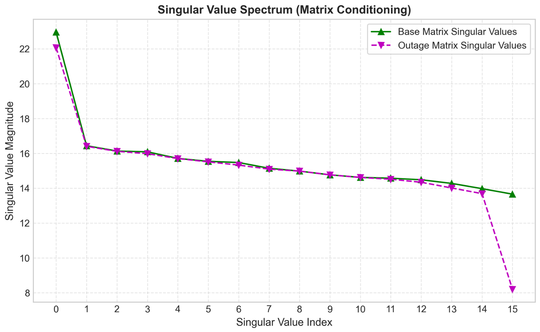
Figure 9 supports the conditioning results in Table 8. The singular values of the two reduced matrices are close over most indices, but the N-1 contingency case exhibits a smaller minimum singular value. This reduction in the smallest singular value increases the condition number from 1.6806 in the base case to 2.6913 in the N-1 contingency case. Therefore, the contingency condition makes the reduced linear system more sensitive to residual and reconstruction errors.

The N-1 contingency case produced a higher condition number than the base case. This indicates that the reduced Jacobian system became more sensitive under the contingency condition. Nevertheless, the obtained condition numbers remained within a moderate range for the examined reduced systems. This helps explain why the VQLS–COBYLA process was still able to reduce the cost in both cases, although a nonzero residual remained.

3.4. Impact of Prescribed V2G Participation on Active Power Losses

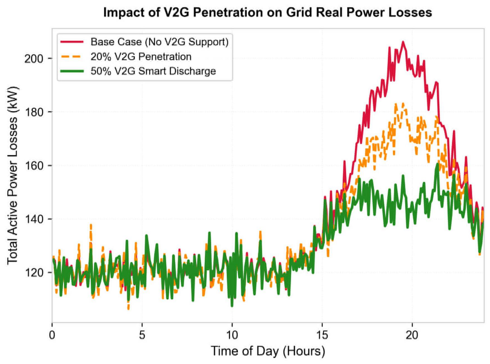
The effect of V2G participation on network active power losses was examined under prescribed support and stress-test scenarios. Figure 10 shows the active power loss trend over the 24-h operating period for the principal V2G participation cases.

During low- and moderate-demand periods, the loss profiles remained relatively close. A clearer difference appeared during the high-demand support period, where V2G active-power injection reduced the upstream feeder power and the corresponding line currents. Because active line losses are proportional to $I^{2}R$, reducing the feeder current leads to lower active power losses.

The V2G scenarios in this study are prescribed operating conditions, not optimized dispatch schedules. Therefore, the V2G support cases should not be interpreted as universally optimal solutions. The loss reduction depends on the assumed load profile, V2G capacity, discharge schedule, connection point, and stress-test condition.

A numerical summary of the loss results is provided in

Table 9. Summary of active power loss results under prescribed V2G participation and stress-test scenarios.

Scenario Description	Reference Loss (MW)	Loss with V2G (MW)	Reduction (%)
S0: Base case without V2G and without contingency	12.45	12.45	0.00
S1: Base case with peak load and V2G discharging	12.45	9.18	26.26
S2: N-1 contingency case without V2G support	18.92	18.92	0.00
S3: N-1 contingency case with V2G emergency support	18.92	13.65	27.85
S4: Dynamic railway-peak loading case with V2G support	21.30	14.80	30.52

. The table includes the base operating condition, a peak-load V2G support condition, an N-1 contingency case, an N-1 contingency case with V2G emergency support, and a dynamic railway-peak loading case with V2G support. These cases are used as prescribed operating conditions for comparison and are not intended to represent a full security-constrained or market-based V2G optimization.

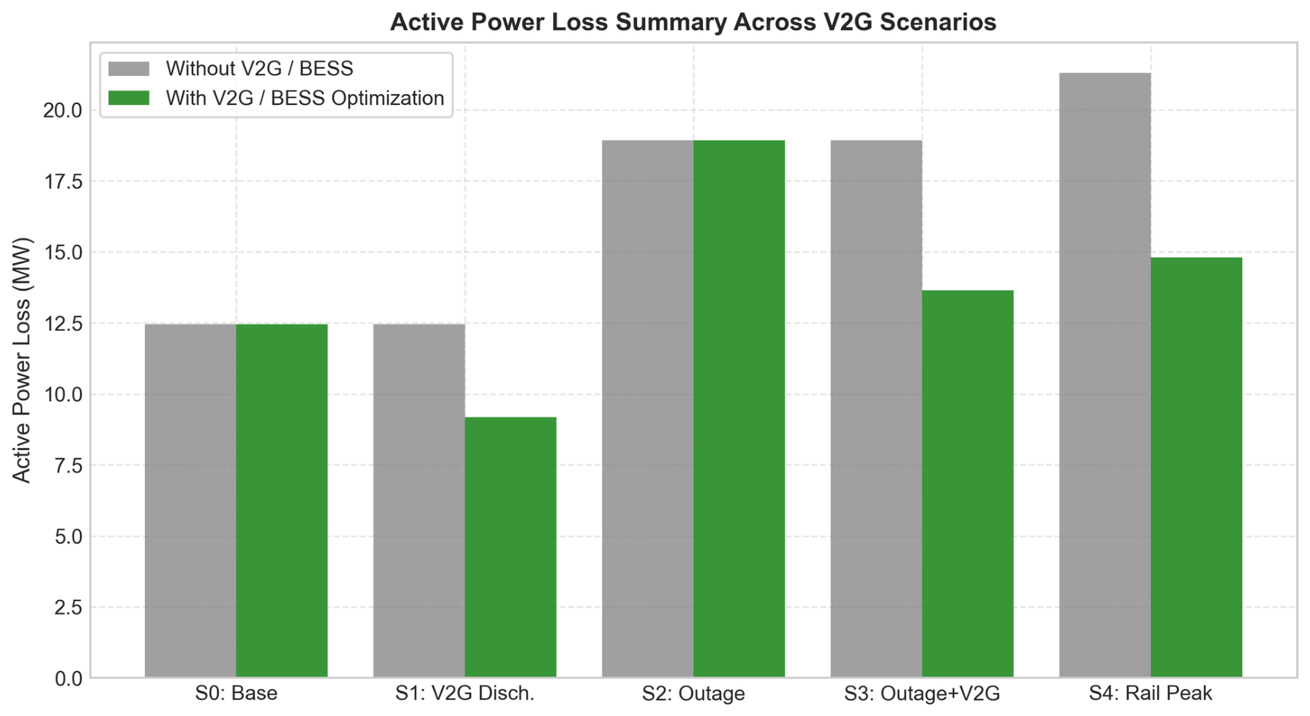
Figure 11 visually summarizes the loss-reduction trend reported in Table 9. No reduction is observed in the base case without V2G support and in the outage case without V2G support. In contrast, the scenarios with V2G support show clear reductions in active power loss. The largest reduction occurs in the dynamic railway-peak loading case with V2G support, followed by the N-1 contingency case with V2G emergency support and the base peak-load case with V2G discharging.

The results show that V2G support reduced the active power loss in the prescribed support cases. Under the base peak-load condition, the active power loss decreased from 12.45 MW to 9.18 MW, corresponding to a reduction of 26.26%. Under the N-1 contingency condition, V2G emergency support reduced the loss from 18.92 MW to 13.65 MW, corresponding to a reduction of 27.85%. The dynamic railway-peak loading case showed the largest reduction among the examined scenarios, decreasing from 21.30 MW to 14.80 MW, or 30.52%.

These results indicate that prescribed V2G active-power support can reduce network losses under both normal and stressed operating conditions. However, the results should not be interpreted as a universally optimal V2G dispatch strategy because the V2G support profiles and operating scenarios were prescribed rather than optimized within a full dispatch framework.

3.5. Additional Fixed-Budget Convergence Assessment

A separate convergence assessment was performed to examine the reduction in the VQLS cost within a fixed budget of 50 optimization iterations. Figure 12 presents the resulting cost trajectory together with the reference tolerance of ${10}^{-4}$.

The cost decreased steadily from a value close to unity at the beginning of the optimization to approximately ${10}^{-2}$ near the end of the 50-iteration period. A substantial reduction occurred during the first 20–30 iterations, after which the rate of improvement became smaller.

Although the cost was considerably reduced, its final value remained above the prescribed tolerance of ${10}^{-4}$. The additional run therefore did not satisfy the tolerance-based convergence criterion within the selected iteration budget. Instead, the result shows that the VQLS–COBYLA procedure progressively improved the candidate solution but would require additional iterations or further adjustment of the circuit and optimizer settings to approach the selected threshold.

Because the main and additional convergence runs used different initial parameter vectors and different iteration budgets, their trajectories were not expected to coincide. The comparison therefore illustrates optimizer sensitivity rather than deterministic convergence to a unique trajectory.

3.6. Repeated VQLS–COBYLA Optimization Runs

To examine reproducibility, repeated independent VQLS–COBYLA runs were performed using the same reduced linear system and circuit configuration but different initial parameter vectors.

Table 10. Statistical summary of repeated VQLS–COBYLA optimization runs.

Metric	Base Case Result	Status
Final cost value, $C_{\mathrm{final}}$	0.081386 ± 0.000310	Stable
Fidelity, F	0.918763 ± 0.000400	High fidelity
Success criterion used in this summary	$C_{\mathrm{final}}<0.10$	Defined threshold
Success rate	100% (30/30 runs)	Passed

summarizes the final-cost and fidelity statistics obtained from the repeated base-case runs.

The repeated-run statistics indicate that the VQLS–COBYLA process produced stable final costs under the selected base-case configuration. The standard deviation of the final cost was small relative to the mean value, suggesting limited variation among the 30 independent runs. The fidelity also remained stable, with an average value of 0.918763. Using the defined success criterion of $C_{\mathrm{final}}<0.10$, all 30 runs satisfied the criterion. These results support the reproducibility of the reduced-system approximation under the selected ansatz, optimizer, and iteration settings.

3.7. Computational Resource-Scaling Trends

Preliminary computational resource trends were examined for systems containing 14, 33, 70, 118, and 300 buses. Figure 13 presents the normalized classical computation index and the VQLS circuit-depth index as the system size increases.

The classical computation index increased markedly with the number of buses. It rose from a relatively small value for the 14-bus case to approximately 4500 for the 300-bus case. The VQLS circuit-depth index also increased with system size, but the plotted increase was more gradual, rising from approximately 50 for the smallest system to slightly above 100 for the 300-bus case.

These trends do not provide a direct comparison of execution time, memory use, total computational cost, or practical scalability. The normalized classical computation index is a dimensionless system-size-based indicator, whereas the VQLS circuit-depth index represents the fitted growth trend of the variational circuit structure. In addition, the plotted circuit-depth index does not include state preparation, matrix encoding, repeated circuit evaluations, measurement operations, classical–quantum communication, classical optimization overhead, Schur-complement construction, or full-state reconstruction.

Therefore, the scaling result should be interpreted only as a comparison of the growth patterns of selected resource indicators. It does not establish quantum speedup, execution-time advantage, or computational superiority over the classical method.

3.8. Overall Numerical Assessment

The combined results provide several complementary observations. First, the main VQLS–COBYLA trajectory shows that the cost can be reduced and stabilized at a small nonzero level for both the base and N-1 contingency cases. Second, the voltage profile obtained using the proposed framework follows the overall behavior of the Newton–Raphson reference solution, while the quantitative metrics provide a clearer measure of the remaining approximation error. Third, the conditioning analysis shows that the N-1 contingency case has a higher condition number than the base case, indicating increased reduced-system sensitivity under the contingency condition.

Fourth, the V2G scenario analysis shows that prescribed V2G active-power support can reduce active power losses under both normal and stressed operating conditions. The largest reported reduction among the examined scenarios was obtained in the dynamic railway-peak loading case with V2G support. Fifth, the additional convergence assessment confirms that a substantial cost reduction does not necessarily imply that a strict tolerance has been reached within a limited number of iterations. Sixth, the repeated base-case optimization results indicate stable final cost and fidelity values under the selected VQLS–COBYLA configuration.

The proposed method requires repeated circuit and cost-function evaluations before returning an approximate correction vector to the classical power flow model. Consequently, the present results do not demonstrate that the hybrid procedure is faster or less computationally expensive than the conventional Newton–Raphson method. The findings should instead be interpreted as a simulation-based proof of concept covering optimization behavior, approximate agreement with the reference solution, V2G-related loss reduction, conditioning effects, reproducibility, and preliminary computational resource trends.

4. Discussion

The revised numerical results provide a clearer basis for interpreting the proposed hybrid quantum–classical framework for power flow analysis. The results show that the VQLS–COBYLA procedure can reduce the residual-based cost of the selected 16 × 16 reduced Jacobian subproblem under both the base operating condition and the N-1 contingency condition. For the base case, the cost decreased from 0.405533 to 0.081386 within 80 COBYLA iterations, whereas the N-1 contingency case decreased from 0.203660 to 0.032900. These results indicate that the variational optimization process was able to improve the candidate solution in both cases. However, the final costs remained nonzero, confirming that the proposed method should be interpreted as an approximate reduced-system solver rather than an exact replacement for a direct Newton–Raphson linear-system solution.

The quantitative accuracy results further support this interpretation. Relative to the Newton–Raphson reference solution, the base case produced a mean absolute error of $8.423265\times {10}^{-2}$, an RMSE of $1.007699\times {10}^{-1}$, a maximum absolute residual error of $2.187494\times {10}^{-1}$, and a cosine similarity/fidelity of 0.918763. The N-1 contingency case produced lower error values, with a mean absolute error of $6.441737\times {10}^{-2}$, an RMSE of $7.668041\times {10}^{-2}$, a maximum absolute residual error of $1.774949\times {10}^{-1}$, and a higher fidelity of 0.952961. These values show that the proposed framework can reproduce the general behavior of the Newton–Raphson solution, but a non-negligible approximation error remains. Therefore, the voltage-profile agreement should be interpreted together with the quantitative error metrics rather than from visual comparison alone.

It should be emphasized that the present IEEE 33-bus demonstration does not represent a complete quantum solution of the full Newton–Raphson Jacobian. The quantum component is limited to a four-qubit representation of a selected 16 × 16 reduced Jacobian subproblem. The remaining state variables are handled through classical reconstruction. Thus, the proposed framework is a hybrid reduced-system implementation, not a full quantum power flow solver for the complete IEEE 33-bus Jacobian. This clarification is important because the computational requirements and numerical behavior of a reduced-system VQLS implementation are different from those of a full-system power flow solver.

The conditioning results provide additional insight into the numerical behavior of the reduced system. The condition number increased from 1.6806 in the base case to 2.6913 in the N-1 contingency case. This increase indicates that the reduced Jacobian became more sensitive under the contingency condition. Nevertheless, the condition numbers remained within a moderate range for the examined reduced systems. This helps explain why the VQLS–COBYLA process was still able to reduce the cost under both operating conditions. In larger or more heavily loaded systems, however, a more poorly conditioned reduced Jacobian could amplify residual and reconstruction errors, making the selection of reduced variables, ansatz depth, and optimizer settings more critical.

The convergence behavior also requires careful interpretation. The main optimization results show cost reduction and stabilization within the prescribed iteration budget, but they do not show exact convergence to a zero residual. The additional fixed-budget convergence assessment similarly showed that the VQLS cost decreased substantially but did not reach the reference threshold of ${10}^{-4}$ within 50 iterations. These findings confirm that cost reduction, cost stabilization, and satisfaction of a strict numerical tolerance are distinct concepts. In the present work, convergence should therefore be understood as stabilization of an approximate variational solution within the available optimization budget.

The repeated-run analysis provides additional evidence regarding the reproducibility of the VQLS–COBYLA process under the selected base-case configuration. Across 30 independent runs, the final cost was 0.081386 ± 0.000310, and the fidelity was 0.918763 ± 0.000400. Using the defined success criterion of $C_{\mathrm{final}}<0.10$, all 30 runs satisfied the criterion. The small standard deviations indicate that the optimizer produced stable results under the selected ansatz, cost formulation, and iteration setting. However, this reproducibility result applies only to the examined reduced system and should not be generalized to all network conditions, larger Jacobian systems, or different ansatz structures without further testing.

The V2G loss results show that prescribed active-power support from the aggregated EV resource can reduce active power losses under both normal and stressed operating conditions. In the base peak-load case, the active power loss decreased from 12.45 MW to 9.18 MW, corresponding to a reduction of 26.26%. Under the N-1 contingency condition, V2G emergency support reduced the active power loss from 18.92 MW to 13.65 MW, corresponding to a reduction of 27.85%. The dynamic railway-peak loading case showed the largest reduction among the examined scenarios, decreasing from 21.30 MW to 14.80 MW, or 30.52%.

These loss reductions are physically consistent with the role of V2G active-power injection in reducing upstream feeder loading. When part of the local demand is supplied by the aggregated EV resource, the current flowing through upstream lines decreases. Since active line losses are proportional to $I^{2}R$, a reduction in feeder current leads directly to lower active power losses. The effect becomes more pronounced under peak-load, contingency, and dynamic stress-test conditions because the feeder current reduction is more significant during these periods.

The V2G scenarios in this work are prescribed steady-state operating conditions, not optimized V2G dispatch schedules. Therefore, the reported loss reductions should not be interpreted as universally optimal V2G strategies. The 20% and 50% participation cases represent prescribed participation levels, and the N-1 and dynamic railway-peak cases are used as stress-test operating scenarios. The results depend on the selected feeder, load profile, V2G connection point, participation ratio, discharge period, and stress-test condition. A different network topology, EV aggregation size, discharge schedule, or V2G location could produce different loss-reduction patterns.

The present V2G model focuses on active-power support and does not optimize reactive-power capability. In practical distribution systems, V2G inverters may provide reactive-power support subject to inverter rating, apparent-power limits, state of charge, vehicle availability, grid-code requirements, and control strategy. Future extensions should therefore include coordinated active- and reactive-power dispatch, Volt–Var control, battery state-of-charge constraints, charging demand, vehicle availability, battery degradation, and market-based or reliability-based V2G scheduling. Such extensions would move the framework from prescribed operating scenarios toward optimized V2G dispatch and responsive setpoint calculation.

The novelty of the present study should be interpreted in this context. The work does not propose a new VQLS algorithm. The VQLS formulation follows the existing variational linear-solver concept introduced in [27]. The main contribution is the engineering integration of a VQLS-based reduced linear-system approximation into a Newton-type AC power flow workflow and the assessment of its behavior under V2G-integrated operating conditions. This positioning is important because the results demonstrate feasibility of integration and numerical behavior, but they do not establish an algorithmic advance over the original VQLS method.

From the quantum-computing perspective, the proposed framework differs from fault-tolerant quantum linear-system algorithms such as HHL and its extensions [22,23]. HHL-type methods provide theoretical relevance for quantum linear-system solving, but their practical use requires demanding assumptions related to state preparation, matrix encoding, sparsity, condition number, controlled operations, and fault-tolerant circuit execution. VQLS is more compatible with NISQ-style workflows [24,26,27], but its performance depends on the ansatz, parameter initialization, optimizer behavior, cost-function evaluation, measurement overhead, and matrix conditioning. QAOA-related approaches are useful for discrete optimization tasks, such as switching, scheduling, and reconfiguration, but they are not direct solvers for continuous Jacobian-based AC power flow equations.

A conceptual comparison among Newton–Raphson, HHL, VQLS, and QAOA is summarized in

Table 11. Conceptual comparison of classical and quantum approaches related to the proposed framework.

Method	References	Role and Relevance to This Study
Newton–Raphson and related classical power flow methods	[13,14]	Established reference methods for nonlinear AC power flow analysis. In this study, Newton–Raphson is used as the numerical benchmark for evaluating the voltage profile obtained from the proposed framework.
HHL-type quantum linear-system algorithms	[22,23]	Provide the theoretical foundation for quantum linear-system solving, but generally require demanding state preparation, matrix encoding, condition number control, and fault-tolerant quantum resources.
VQLS and related variational linear-system solvers	[27,29,30]	Offer a NISQ-oriented approach for approximating linear-system solutions. Their performance depends on the ansatz, optimizer, initialization, conditioning, and cost-evaluation overhead.
QAOA and quantum alternating-operator approaches	[31,32]	Useful for variational optimization problems such as scheduling, switching, or reconfiguration, but not a direct solver for continuous Jacobian-based AC power flow equations.
Proposed framework	This work	Integrates VQLS into a reduced Newton-type AC power flow workflow by solving a selected 16 × 16 reduced Jacobian subproblem and reconstructing the complete correction vector classically. The framework is presented as a simulation-based proof of concept for a V2G-integrated distribution system.

. This comparison is included to clarify the role of the proposed method relative to classical and quantum approaches rather than to claim superiority over any of them.

The resource-scaling result should also be interpreted cautiously. The normalized classical computation index increased markedly from the 14-bus case to the 300-bus case, while the VQLS circuit-depth index showed a more gradual increase over the same range. However, these indicators do not represent the same physical quantity. The classical index is a dimensionless system-size-based indicator, whereas the VQLS index represents a fitted circuit-depth trend. Therefore, the observed difference in growth pattern does not demonstrate execution-time advantage, practical scalability, or quantum speedup.

In addition, the VQLS circuit-depth index does not include state preparation, Jacobian encoding, right-hand-side preparation, repeated circuit executions, measurement shots, cost-function estimation, classical–quantum communication, COBYLA optimizer overhead, Schur-complement construction, or classical full-state reconstruction. A complete computational comparison would require both the classical and hybrid quantum–classical methods to be evaluated under common accuracy criteria, common stopping conditions, and comparable implementation conditions. Runtime, memory use, number of circuit evaluations, number of measurement shots, optimizer evaluations, hardware latency, solution accuracy, and reconstruction error would all need to be included.

Compared with established power flow techniques, the proposed framework still introduces considerable computational overhead. Newton–Raphson and fast-decoupled methods are mature, efficient, and widely implemented [13,14]. They are also readily available in practical platforms such as Pandapower [18]. The VQLS framework adds an inner optimization loop requiring repeated circuit and cost-function evaluations before an approximate correction vector is returned to the classical power flow model. Accordingly, the present contribution lies in demonstrating the feasibility of the computational integration rather than improving present-day solution speed.

Simulation using an ideal statevector backend does not represent the full behavior of a physical NISQ processor. Gate noise can distort the prepared variational state, measurement errors can bias the estimated cost, limited qubit connectivity can increase circuit transpilation depth, and finite-shot sampling can introduce statistical fluctuations into the optimizer feedback. These effects may slow convergence, increase residual error, or cause optimizer stagnation. Therefore, noisy simulation, error mitigation, and hardware experiments are important next steps before the approach can be assessed under realistic quantum-device conditions [33,34].

Several limitations should therefore be recognized. First, the detailed power flow and voltage comparison was conducted using a reduced 16 × 16 Jacobian subproblem represented by four qubits. This reduced implementation does not yet demonstrate a complete quantum representation of the full IEEE 33-bus Jacobian system. Second, the quality of the result depends on the fixed variable selection, reduced-system conditioning, ansatz expressibility, and optimizer configuration. Third, the V2G scenarios were prescribed rather than optimized. Fourth, the N-1 contingency and dynamic railway-peak cases were used as stress-test operating scenarios and should not be interpreted as a complete security-constrained or railway-load optimization framework.

Fifth, the resource-scaling assessment used selected benchmark sizes only to illustrate resource-indicator trends. It was not a full VQLS validation for all examined systems and did not include total execution time or complete quantum-hardware overhead. Sixth, the present implementation used an ideal statevector simulator and therefore did not include gate noise, finite-shot uncertainty, limited connectivity, readout error, or hardware queue and communication delays.

A technical roadmap toward a more practically relevant quantum-enhanced power flow solver would require progress in several areas: more efficient Jacobian and right-hand-side encoding, improved reduced-system or full-system state preparation, ansatz designs matched to power-flow Jacobian structure, robust optimizers with reduced sensitivity to initialization, noise mitigation for residual-cost estimation, systematic conditioning-aware variable selection, and hardware platforms with sufficient qubit counts, connectivity, gate fidelity, and circuit depth. In addition, future studies should compare hybrid quantum–classical solvers and classical solvers under common accuracy, runtime, and resource-accounting criteria.

Overall, the study should be regarded as a proof-of-concept contribution to quantum-assisted power system analysis. The results show that a VQLS–COBYLA procedure can be integrated into an iterative AC power flow framework and can produce an approximate reduced-system solution that follows the general behavior of the Newton–Raphson reference. The additional analyses clarify the role of reduced Jacobian conditioning, the stability of repeated optimization runs, the potential of prescribed V2G support to reduce active power losses under selected operating conditions, and the limitations of resource-indicator comparisons. However, no superiority over classical methods or quantum computational speedup is established.

Future work should include complete Jacobian representations, alternative reduced-variable selection strategies, conditioning-aware system reduction, repeated optimization under different operating points, alternative ansatzes and optimizers, quantitative comparisons using common accuracy thresholds, noisy simulation environments, and implementation on available quantum processors. The V2G model should also be extended to include different V2G locations, multiple participation levels, active- and reactive-power control, battery state-of-charge constraints, vehicle availability, charging demand, battery degradation, and optimized V2G dispatch under realistic distribution-network operating conditions.

5. Conclusions

This study presented a simulation-based hybrid quantum–classical framework for steady-state AC power flow analysis in a distribution network with vehicle-to-grid (V2G) integration. In the proposed procedure, the nonlinear AC power flow equations are linearized iteratively, and a Variational Quantum Linear Solver (VQLS) is used to approximate the resulting reduced Jacobian-based linear system. The parameters of the variational circuit are updated using the COBYLA optimizer, after which the reconstructed state-correction vector is returned to the classical power flow model.

The contribution of this work does not lie in proposing a new VQLS algorithm. Rather, it lies in the engineering integration of an existing VQLS formulation into a reduced Newton-type AC power flow workflow and in the assessment of its numerical behavior under prescribed V2G operating scenarios.

The detailed proof-of-concept evaluation was conducted using a modified IEEE 33-bus radial distribution system with an aggregated V2G unit connected at Bus 18. The quantum component represented a selected 16 × 16 reduced Jacobian subproblem using a four-qubit Real-Amplitudes circuit, while the remaining state variables were recovered through classical reconstruction. Therefore, the proposed implementation should be interpreted as a hybrid reduced-system approach rather than a complete quantum solution of the full IEEE 33-bus Newton–Raphson Jacobian.

In the main optimization run, the VQLS cost decreased substantially during the early iterations and subsequently approached a nearly stationary nonzero level. The resulting bus-voltage profile followed the overall behavior of the Newton–Raphson reference solution, although small differences remained because of the approximate nature of the variational solution. The additional 50-iteration convergence assessment reduced the cost from a value close to unity to approximately ${10}^{-2}$, but the reference tolerance of ${10}^{-4}$ was not reached within the available iteration budget. This result confirms that cost stabilization should not be regarded as equivalent to satisfying a strict numerical tolerance.

The revised evaluation also emphasizes the need for quantitative accuracy and residual metrics when interpreting the voltage-profile comparison. Voltage-error indices, reduced-system residual norms, post-update power mismatches, and the condition number of the reduced Jacobian provide a more rigorous basis for assessing the numerical consistency of the proposed method relative to the Newton–Raphson reference solution.

The V2G scenario analysis showed that prescribed active-power support from the aggregated EV resource can reduce active power losses under the selected normal and stressed operating conditions. The reported loss reductions were 26.26% for the base peak-load case with V2G discharging, 27.85% for the N-1 contingency case with V2G emergency support, and 30.52% for the dynamic railway-peak loading case with V2G support. However, these results should not be interpreted as universally optimal V2G strategies because the V2G support profiles and operating conditions were prescribed rather than optimized.

The preliminary resource-scaling assessment showed different growth patterns for the normalized classical computation index and the VQLS circuit-depth index as the system size increased from 14 to 300 buses. Because these indicators represent different computational quantities, the result does not provide a direct execution-time comparison and does not establish quantum speedup, computational superiority, or practical scalability over established classical power flow methods.

Several limitations should be recognized. The present implementation used an ideal statevector simulator and therefore did not include gate noise, finite-shot uncertainty, readout error, limited device connectivity, or physical quantum-hardware execution overhead. In addition, the V2G model did not include battery state of charge, vehicle availability, inverter reactive-power capability, charging behavior, battery degradation, or market-based dispatch.

Overall, the results support the numerical feasibility of incorporating a VQLS-based approximation into an iterative AC power flow procedure under a reduced and ideal simulation setting. The study demonstrates how a hybrid quantum–classical solver can be examined together with V2G operating scenarios, convergence behavior, voltage-profile agreement, reduced-system conditioning, and preliminary resource indicators. Nevertheless, the present work remains a proof-of-concept study and does not claim replacement of mature classical solvers.

Future work should consider full-system Jacobian representations, conditioning-aware variable selection, repeated optimization runs with different initial parameters, alternative ansatzes and optimizers, noisy simulation environments, and implementation on available quantum processors. Further extensions should also include different V2G locations, multiple participation levels, active- and reactive-power control, battery state-of-charge constraints, vehicle availability, and optimized V2G dispatch under realistic distribution-network operating conditions.