


Abstract
Increasing variability in electricity load patterns, driven by end-use behaviour, grid-related technological changes, and socio-economic factors, calls for more accurate and efficient short-term load prediction (STLP) models. This study evaluates the predictive performance of four hybrid models for short-term Amp-load prediction: Adaptive Neuro-Fuzzy Inference System (ANFIS) combined with Genetic Algorithms (GA) and Particle Swarm Optimisation (PSO), as well as convolutional neural networks (CNN) integrated with long short-term memory (LSTM) and extreme gradient boosting (XGB). The models were developed using hourly Amp-load data collected from a power utility substation in Kenya, together with corresponding meteorological data (temperature, wind speed, and humidity) covering a period from January 2023 to June 2024. Results show that the ANFIS-PSO and ANFIS-GA models outperform the CNN-based models, achieving MAPE values of 4.519 and 4.363, RMSE values of 0.3901 and 0.4024, and R2 scores of 0.8513 and 0.8481, respectively, due to the adaptive nature of ANFIS, which enables effective modelling of the irregular, nonlinear, and complex temporal behaviour of the Amp load. Enhanced prediction accuracy was observed across all models when variational mode decomposition (VMD) was applied to pre-process the input data. This result was corroborated through further analysis of the Amp-load signals using Taylor plots. Among all of the configurations tested, the CNN-LSTM-VMD model exhibited the highest overall prediction accuracy, with MAPE of 2.625, RMSE of 0.1898, and R2 of 0.9702, marginally outperforming the ANFIS-PSO-VMD model, thus making it more suitable for short-term load prediction applications.
1. Introduction
1.1. Context of Short-Term Load Prediction
Accurate and efficient short-term electrical load prediction (STLP) plays a vital role in ensuring reliable power system operation and cost-effective energy dispatch. Moreover, as power grids increasingly integrate variable renewable energy from non-dispatchable energy sources, along with smart metering infrastructure and electric mobility systems, the importance of accurate STLP has become even more apparent. Errors in short-term electric load predictions can significantly affect the availability of generation units, unit commitment, economic dispatch of scheduled units, spinning reserve allocation, as well as overall system losses and stability margins [1].
A load in an electrical grid can be measured as apparent power (KVA) or inferred from line current at a transformer or feeder at a given operating voltage and power factor (Amp load). Therefore, the profile of Amp load follows the pattern of power consumption of a network. Normally, power is transmitted from the generating units to substations at high voltage, then distributed from substations to transformer stations at medium voltage. According to the IEC 60038 standard, medium voltage (MV) is defined as voltages from over 1 KV to 35 KV.
The available literature over an eight-year period (2015–2022) indicate that 54% of electricity load prediction studies relied on weather, time and economic factors, whereas the remaining 46% focused on household behaviour patterns and historical energy consumption data [2,3,4,5,6,7]. This distribution highlights the methodological acceptance and feature importance of weather features and historical load in future load prediction modelling. Time-related effects include calendar parameters such as the day of the week and hour of the day, as well as seasonal influences like calendar holidays. Variations in electric load demand over time are periodic and mirror human activity patterns, including work routines, social time, and sleeping cycles. These time effects became strongly evident during the early COVID-19 period when most industrial and commercial units closed or operated on reduced capacities, leading to noticeable changes in load demand levels, alongside a shift in domestic electricity consumption driven by the widespread adoption of the ‘work-from-home’ policy. Weather is often considered a pivotal point that can lead to power system unreliability by lowering power supply efficiency [8]. For countries around the Equator, the weather factors that are widely used for STLP include temperature, humidity and wind speed. The accuracy of STLP can be enhanced by employing hybridized forecasting models with the integration of weather variables, historical load data and time-based factors. Despite being a widely researched area of study, there remains some open questions that need further research, such as the optimality of input data and the hybridization approach.
In this paper, the STLP performance of hybridized machine learning (ML) models based on artificial neural networks, decision tree ensembles and a fuzzy inference system approach with different learning algorithms and data decomposition are evaluated and compared. The results can provide decision-makers with valuable insights towards improving the choice of ML optimization algorithms and hybridization approach for STLP applications. Therefore, the primary contributions and novelty of this study are summarized as follows:
- The study provides a comparative benchmark for medium-voltage Amp-load forecasting under consistent hybridization and variational mode decomposition (VMD) pre-processing.
- Dual-stage evaluation of the performance of the hybridized ML models on both training and testing datasets provides enhanced understanding of the models’ performance characteristics and valuable insights for practical applications.
1.2. Short-Term Load Prediction Techniques
Short-term electricity demand prediction has been widely investigated, with existing methods in the literature commonly grouped into two broad categories: statistical (time-series) methods and machine learning (artificial intelligence) approaches. Statistical methods model electricity demand by capturing trends and seasonal patterns using historical data. However, a fundamental limitation of these methods is their inability to effectively represent the complex and nonlinear relationships between future electricity demand, past load behaviour, and meteorological variables, which often results in reduced prediction accuracy [1]. To address the challenges of statistical methods, machine learning (ML) methods have been widely utilized for short-term electricity demand predictions. ML approaches employ diverse optimization techniques to model nonlinearities and enable adaptive learning without requiring prior assumptions about load–weather relationships. ML algorithms are trained based on available data to generate an outcome by supervised or unsupervised learning.
Recent studies in the literature on STLP have predominantly employed individual machine learning (ML) techniques using weather data, time factors and past load data as predictors [9,10,11,12,13]. While the individual ML models achieved acceptable accuracy, they tended to overfit or underfit especially where the data was noisy. Indeed, it is noteworthy that each individual ML method has some inherent deficiencies and their performance varies under different conditions, which poses limitations in practical applications. In order to address the limitations of individual ML methods and improve the efficiency and accuracy of the predictions, several studies have proposed hybridization of ML techniques. As reported in the literature [2,14,15,16,17,18,19,20] different hybrid ML-based models for electrical load prediction consistently improved the prediction accuracy by almost 3.5% compared to the closest-performing individual model. From this finding, it is apparent that the hybridization of ML-based techniques is the best approach to improve prediction accuracy. While the improvement may appear marginal, in power system forecasting even small percentage reductions in error translate into significant economic benefits. In this study, the predictive capability of four hybrid machine learning models is comparatively evaluated. The models comprise an adaptive neuro-fuzzy inference system (ANFIS) combined with Particle Swarm Optimization (PSO), an ANFIS combined with Genetic Algorithms (GAs), convolutional neural networks (CNN) coupled with a long short-term memory algorithm (LSTM), and CNN integrated with an extreme gradient boosting (XGB) machine.
2. Machine Learning Methods for STLP
The basics and structure of the algorithms for each of the proposed ML models are presented and discussed here. However, the detailed mathematical theory of these models is widely available in the literature and will not be presented in this paper.
2.1. Convolutional Neural Networks (CNN)
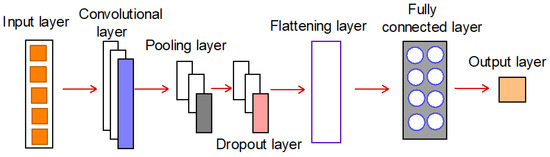
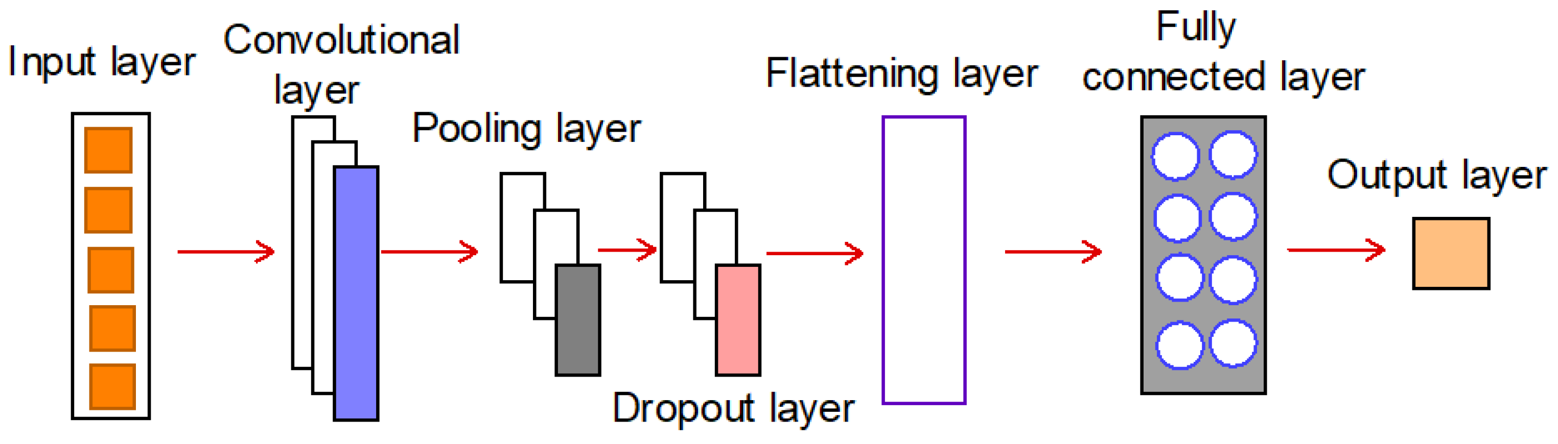
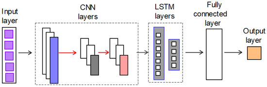
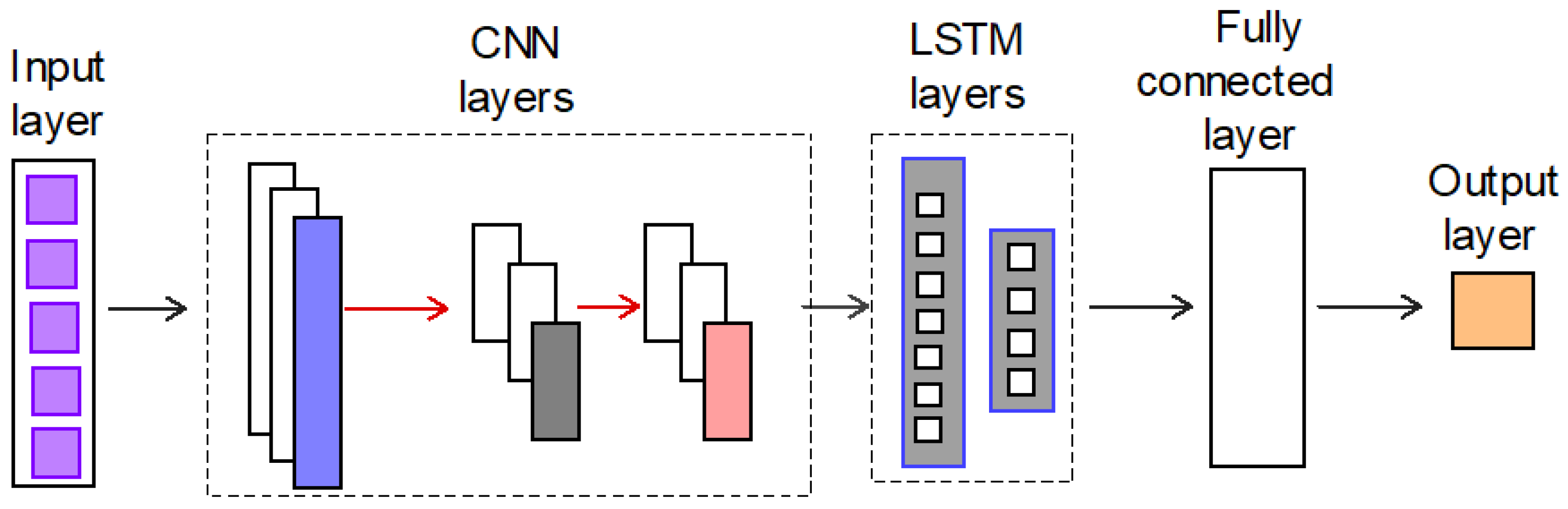
A CNN is a deep neural network technique with the capability to extract local trends from contiguous data [21]. Figure 1 adapted from Tudose et al. 2021 [21] is a schematic representation of the structure of CNN model.
Figure 1.
Schematics of typical CNN model structure.
The input layer accepts the input data and passes it to the subsequent layers. The convolution layer applies a set of filters/kernels to the input data to extract features from the data. Considering a one-dimensional input, the convolution operation can be described by the following equation:
where represents the convolution operator, while I and K are the one-dimensional input and the kernel, respectively. The output of the convolution operation is the feature map.
A nonlinear activation function is applied to the output of the convolutional layer to introduce nonlinearity into the network. The pooling layer reduces the spatial size of the feature maps generated by the convolutional layer by down-sampling them, i.e., it extracts the maximum or average value of adjacent elements from a feature map. The dropout layer randomly drops out some of the neurons in the network by randomly setting a fraction of the activations to zero during training to prevent overfitting. The flatten layer converts the multi-dimensional feature maps generated by the previous layers into a one-dimensional vector that can be passed to a fully connected layer. The fully connected layer connects every neuron in the previous layer to every neuron in the current layer, while the output layer produces the final output of the network. However, it is noteworthy that the number of layers and their configuration in the CNN model depends on the characteristics of the input data.
2.2. Long Short-Term Memory (LSTM)
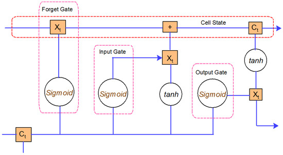
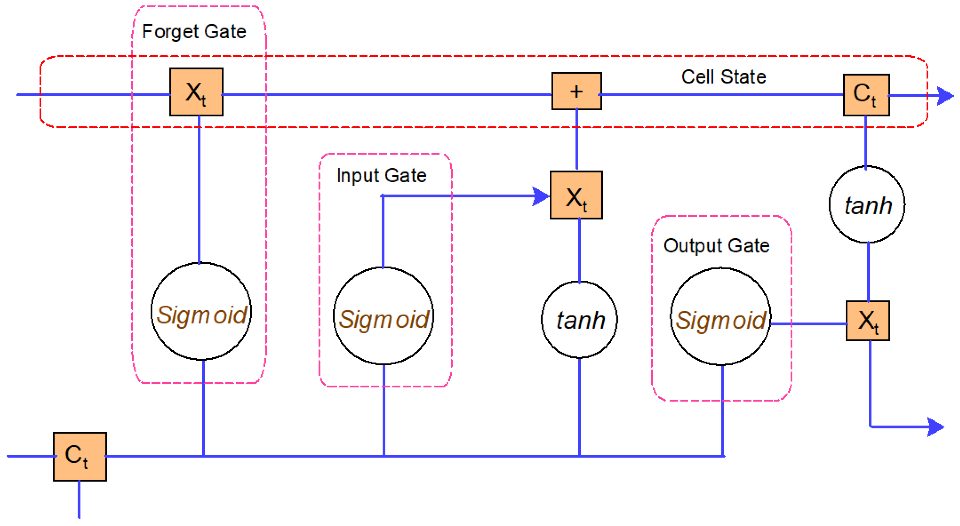
LSTM models are extensions of recurrent neural networks (RNNs) that can handle sequential data. LSTM models were developed to overcome the vanishing and exploding gradients problem, which occurred with conventional RNNs when processing information that requires long-term or short-term dependencies. They have memory cells and gates that allow them to selectively remember or forget information from previous time steps. The fundamental structure of an LSTM module consists of three logistic sigmoid gates and one tanh layer as displayed in Figure 2 [19]. Each one of these gateways takes on a state variable at a particular time phase.
Figure 2.
Fundamental structure of LSTM model.
The input gate uses a sigmoid function to control information that is passed from the current input and the previous hidden state into the memory cell while the forget gate decides how much information from the previous memory cell enters the current memory cell. The memory cell is the internal state of the LSTM. The output gate uses the sigmoid function and tanh function to control the flow of information from the memory cell to the current hidden state and output [16]. The study by Muzaffar and Afshari [22] revealed that the LSTM model has the potential to predict electric demand load for short time horizons. The main drawback of an LSTM is the tendency to overfit and the difficulty with applying a regularization technique to curb this issue. Combining LSTMs with other deep neural networks like CNNs can mitigate the shortfall and improve the quality of predictions as demonstrated in the work by Guo et al. [23].
2.3. Adaptive Neuro-Fuzzy Inference System (ANFIS)
ANFIS is a hybrid system of neural networks and fuzzy systems, with the ability to make fuzzy logic decisions with neural network computational capability. The fuzzy system component defines the membership functions while the neural network component is used to automatically extract fuzzy IF-THEN rules from numerical data and adaptively tunes the parameters of the membership function through a hybrid learning process [24]. A membership function maps crisp input values to a fuzzy degree (between 0 and 1), indicating how much the input belongs to a fuzzy set as described by Equation (2), where µA(x) is the membership value, x is the input value and A is a fuzzy set. This approach leverages the trainability of neural networks and the high decision-making power of fuzzy systems in conditions of uncertainty and certainty.
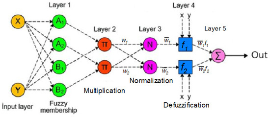
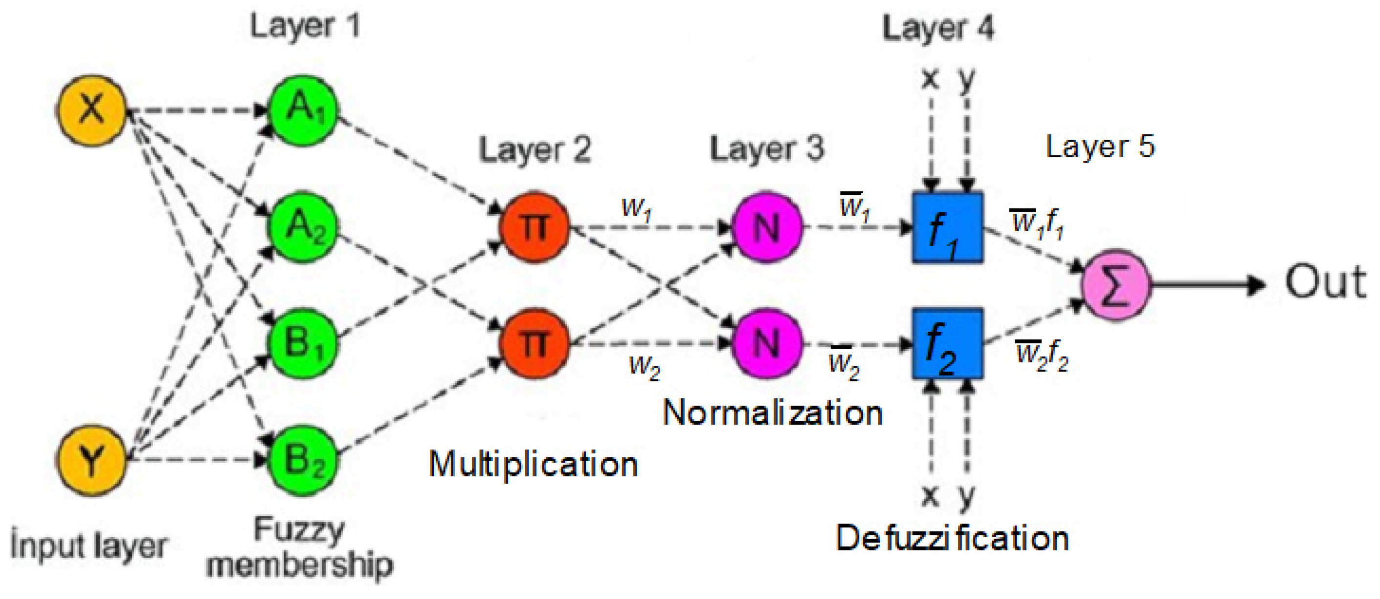
Considering a first-order Sugeno fuzzy model with two inputs x and y and one output f, a rule set with two fuzzy if–then rules can be expressed as shown in Equations (2) and (3), in which p1, q1, and r1 and p2, q2, and r2 denote consequent parameters learned during training, and A1, A2, B1, and B2 are fuzzy membership functions [25,26]:
Rule 1: IF (x = A1 and y = B1) THEN (f1 = p1x + q1y + r1)
Rule 2: IF (x = A2 and y = B2) THEN (f2 = p2x + q2y + r1)
The equivalent ANFIS network structure can be described by Figure 3, which comprises five layers. Layer 1 is the input or fuzzification layer that converts numerical inputs into fuzzy values using membership functions. Layer 2 is the rule layer that applies fuzzy inference rules to model relationships in the data. Layer 3 is where normalization is performed using the weights of all neurons in the layer, ensuring the rule strengths sum to 1. Defuzzification occurs in layer 4 converting fuzzy output into a crisp predicted value while the final output is produced in Layer 5.
Figure 3.
The structure of the ANFIS network.
2.4. Genetic Algorithms (GAs)
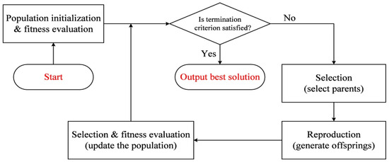
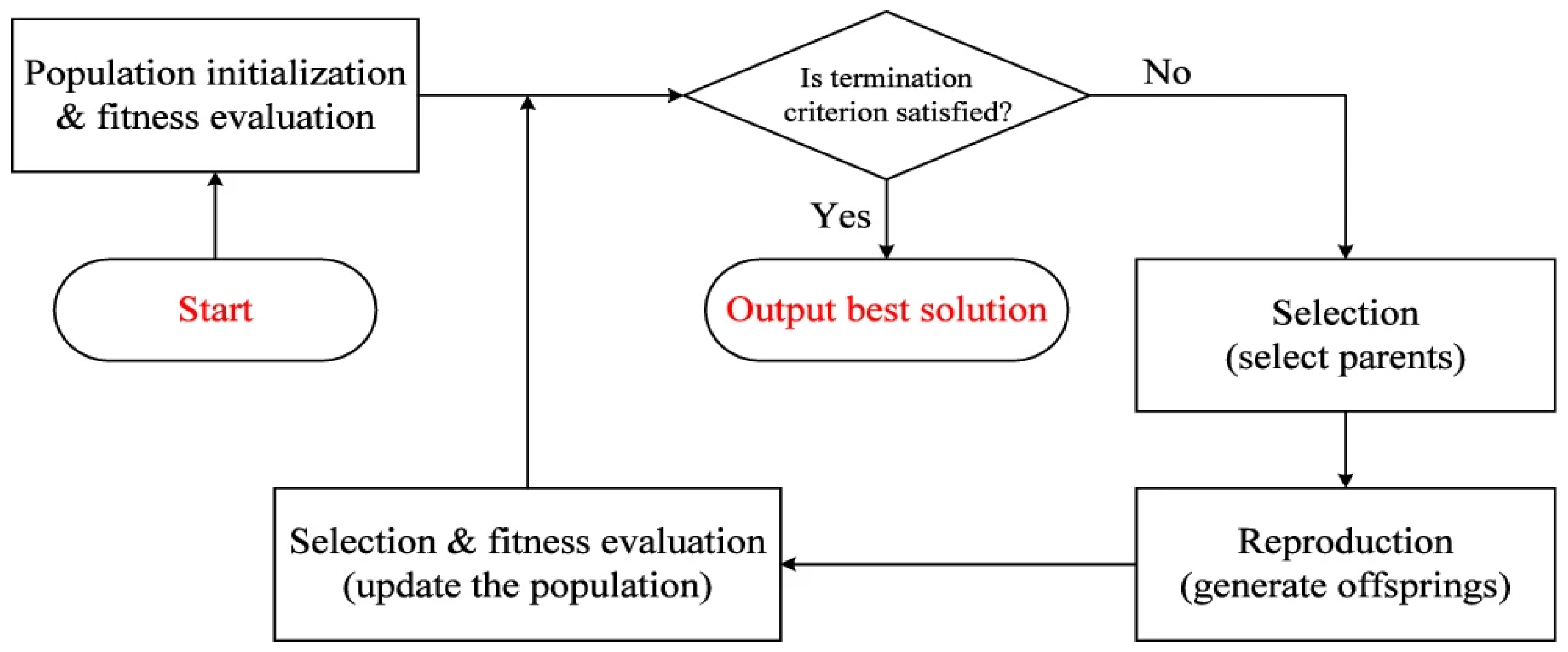
A genetic algorithm (GA) is a search-based algorithm for solving constrained and unconstrained optimization problems based on principles inspired by natural genetics to evolve solutions to problems. The basic idea is to maintain a population of chromosomes that represents candidate solutions to a problem, and the candidate will evolve over a period of time through competition and controlled variation. Details of the GA framework can be reviewed in the work by Katoch et al. [27] and other studies available in the literature. Figure 4 is a flowchart of a GA solution search process. The algorithm terminates when either a maximum number of generations has been produced, or a satisfactory fitness level has been reached for the population.
Figure 4.
Flowchart of the general framework of a GA solution search.
Ray et al. [28] successfully applied a GA to obtain the optimal parameters for an LSTM model, which was then applied to predict the hourly electricity load using hourly weather data obtained from the Australia Bureau of Meteorology and hourly electricity load data obtained from the Australian Energy Market Operator. Also, Santra and Lin [29] used a hybrid model with LSTM and a GA to predict hourly to daily electricity load one hour to one week ahead, with good accuracy.
2.5. Particle Swarm Optimization (PSO)
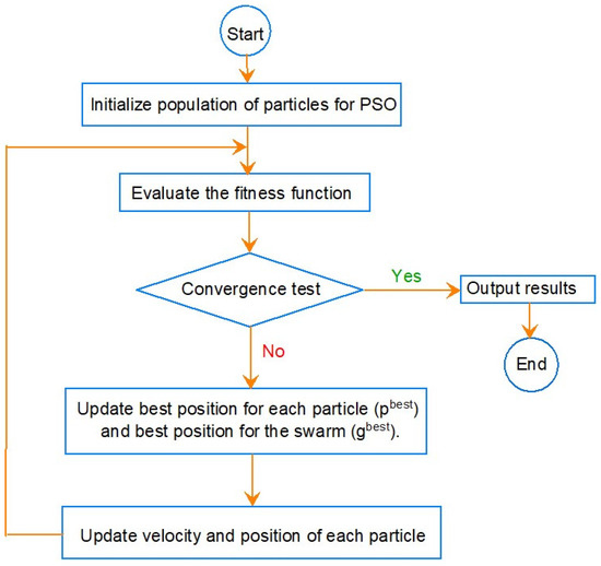
PSO is a collective intelligence algorithm based on the concept of swarm intelligence, with ability to perform a global search and optimization [24]. A population of random solutions is used to initialize the PSO algorithm and the search for an optimal solution is done by updating the positions of the particles at each successive iteration. PSO scatters a population (swarm) of candidate solutions (particles in a swarm), and the movement of each particle is affected by its best position and the best position of the swarm. The basic structure of the PSO algorithm in shown in Figure 5. Details of the governing equations for PSO algorithms are widely available in the literature and will not be repeated here. PSO has been used by different researchers to improve the performance of artificial neural network models in various prediction applications. Ozerdem et al. [30] used PSO for short-term electric load forecasting. The results obtained showed that the PSO-optimized feedforward networks are suitable regressors for modelling energy demand. In another study, Chafi and Afrakhte [31] applied a deep neural network and PSO in short-term load forecasting, achieving fast convergence and a relatively low mean absolute error. This was further explored by Hong and Chan [32], who combined PSO and a CNN to study hourly load data in Taiwan Power Company. The simulation results indicated better predictive performance in comparison to an Autoregressive Integrated Moving Average model, which underscores the merits of PSO.
Figure 5.
Particle swarm optimization (PSO) algorithm.
2.6. Extreme Gradient Boosting Tree Ensemble (XGB)
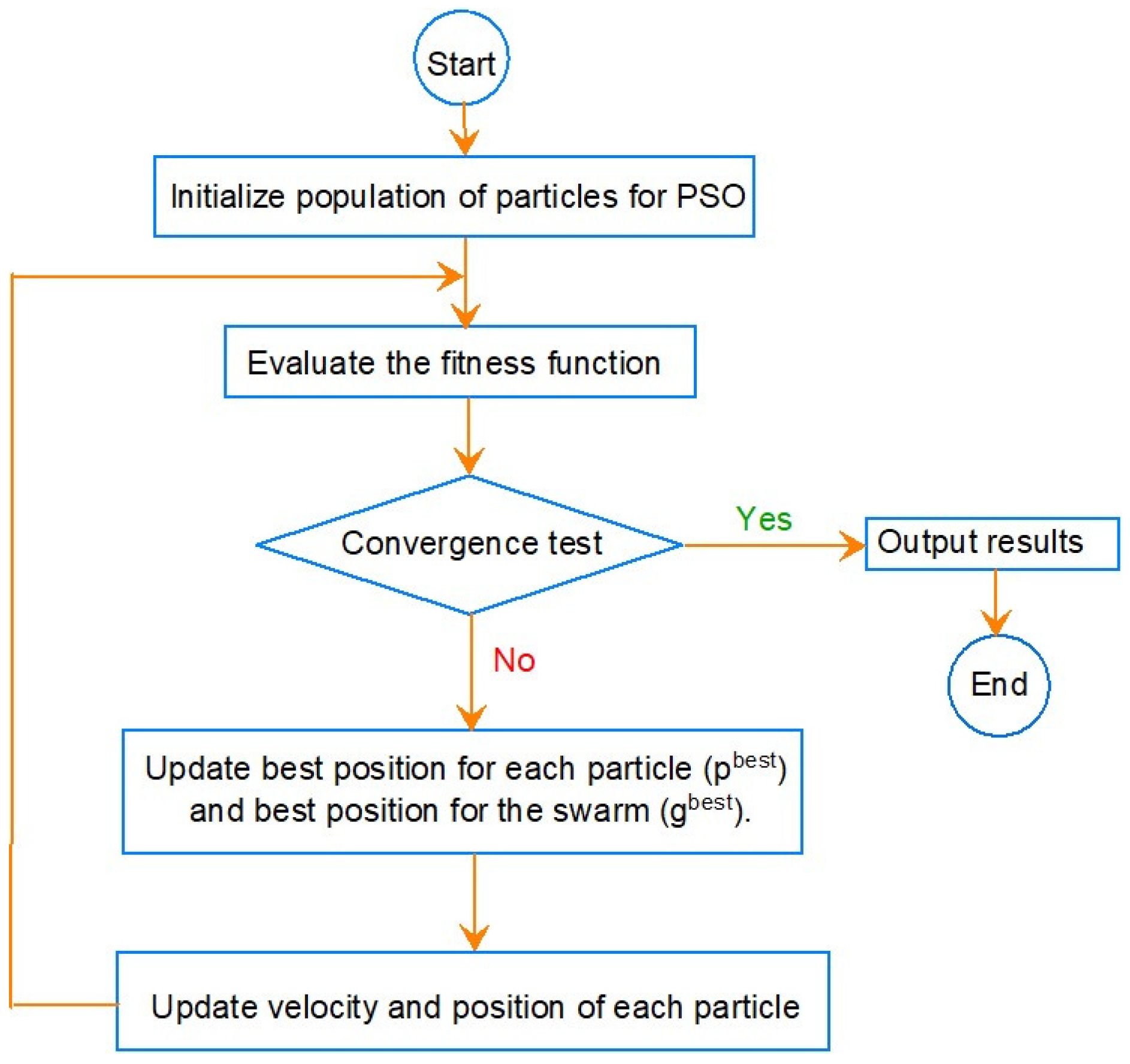
A decision tree ensemble model is a machine learning method that combines multiple decision trees to make better and more generalized predictions. Each decision tree in the ensemble takes input data and splits it into smaller groups based on different features. Each split creates branches and at the end of these branches are the predictions. The ensemble combines all these individual predictions to make a final, more accurate prediction [33,34]. Figure 6 represents the structure of the XGBTE search algorithm.
Figure 6.
Structure of the XGBTE search and prediction algorithm.
Gradient boosting builds an ensemble of decision trees sequentially such that the set target outcomes are dependent on the gradient of the error versus the prediction. Each new tree model added to the ensemble tries to correct the errors made by previous ones. At the m-th iteration, a simple tree model hm(x) is added to the previously built overall model, and it is fitted to predict the residuals of the model Hm−1(x) available from the previous (m − 1)-th iteration, giving a new prediction model, Hm(x). The parameter η is the learning rate (scaling factor).
The final prediction is the weighted sum of the predictions from all of the trees. A loss function is optimized using the gradient descent method, reducing errors iteratively. One drawback of this technique is the possibility of the solution becoming too complex and overfitting the data, leading to poor generalization. To optimize the performance, it is essential to tune the hyperparameters (number of trees, learning rate, tree depth, minimum samples per leaf and shrinkage).
3. Materials and Methods
3.1. Hybridization of the Models
This study explores the hybridization of machine learning (ML) models and the application of different learning and optimization algorithms in short-term electric load prediction to overcome the limitations inherent in individual ML algorithms. Four different hybrid ML models are evaluated, namely CNN-LSTM, CNN-XGB, ANFIS-PSO, and ANFIS-GA. The basics and structure of the algorithms for each of these models are presented and discussed in the sections that follow.
3.1.1. CNN-LSTM
The structure of the CNN-LSTM model assessed here involves convolutional neural network (CNN) layers for feature extraction (spatial and local temporal patterns) on input data combined with LSTMs to support learning and Amp-load prediction. The LSTM uses cells and gates to regulate information flow through the network, and can memorize information over longer sequences, thereby overcoming the vanishing gradient problem. Figure 7 illustrates the algorithm for the CNN-LSTM model implementation. A rectified linear unit (ReLU) activation function has been used for each convolutional and fully connected layer.
Figure 7.
Flowchart of the algorithm for the integrated CNN-LSTM Model.
3.1.2. CNN-XGB
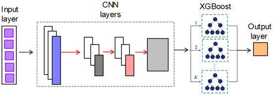
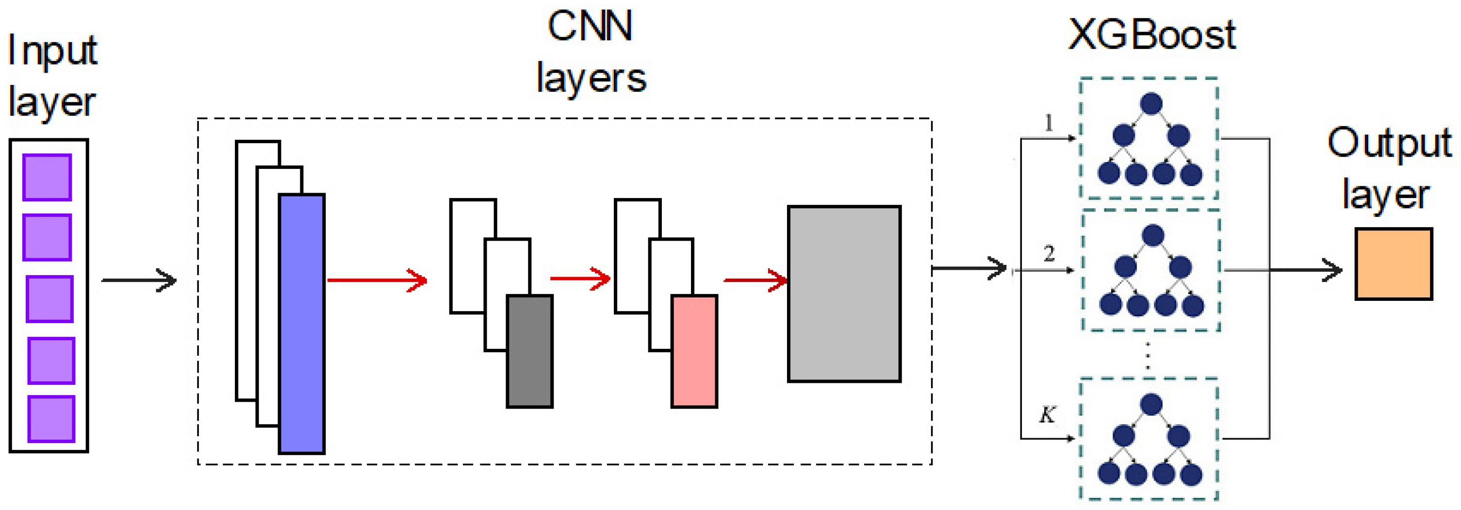
The hybrid model of a CNN combined with XGB leverages both deep learning and ensemble learning for robust short-term load prediction. The CNN component extracts features (captures spatial dependencies) from historical load data and other input variables using convolutional layers. The extracted feature maps are flattened into feature vectors. The feature vectors are passed into XGB, which builds multiple decision trees and optimally weights them using gradient boosting. The trained model predicts the short-term electricity load using the optimized tree ensemble where each decision tree casts a vote and the ensemble predicts the majority vote of all of its trees. Figure 8 is a schematic representation of the training and prediction algorithm.
Figure 8.
Flowchart of the algorithm for the integrated CNN-XGB model.
3.1.3. ANFIS-PSO
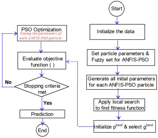
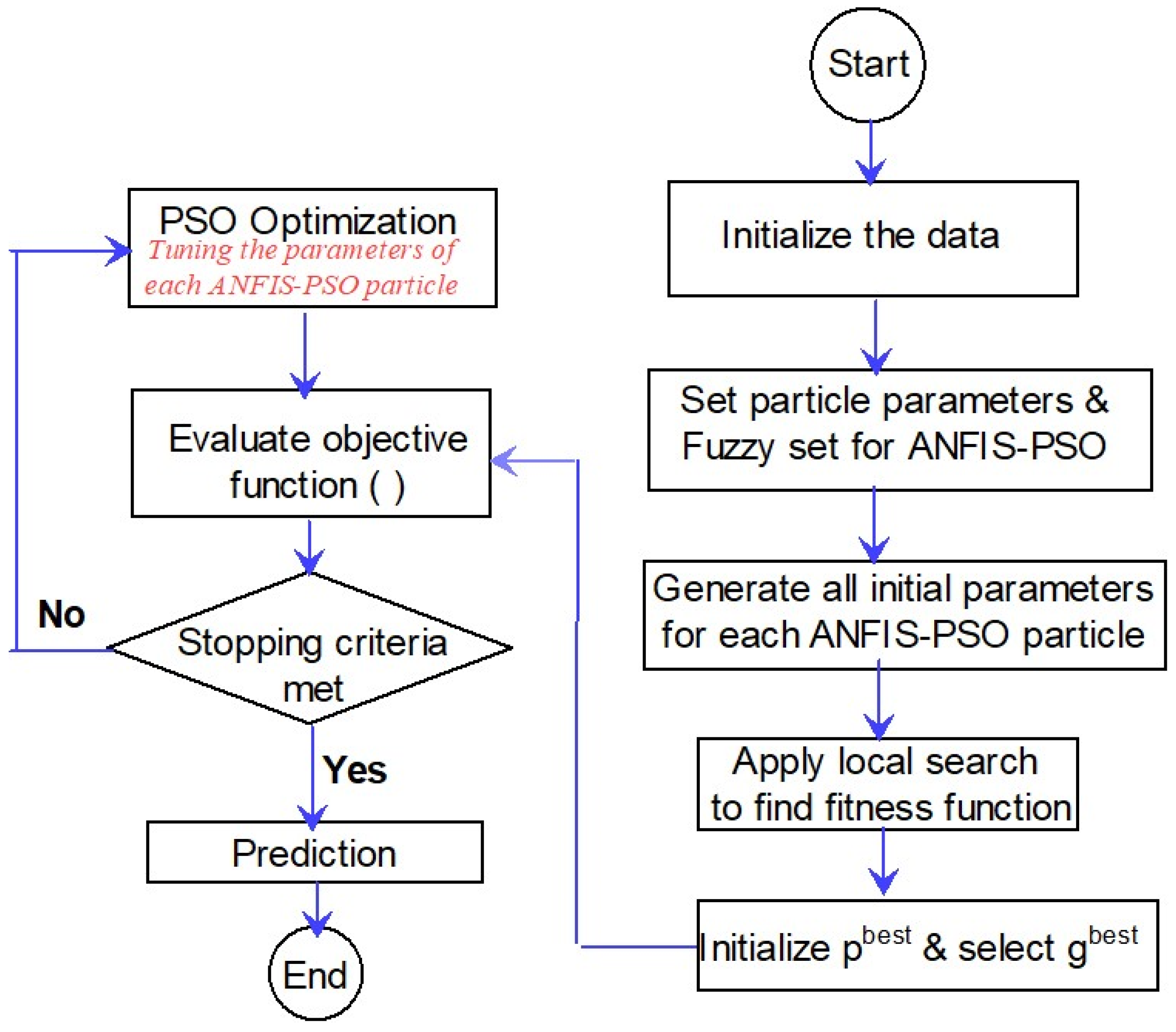
The ANFIS-PSO system combines metaheuristic optimization and fuzzy logic-based modelling for accurate short-term load prediction. In this study, the ANFIS was initialized with fuzzy membership functions and inference rules to predict the Amp load through adaptive learning. The Gaussian membership function was used because it is smooth and differentiable and provides better adaptability for machine learning models. The optimized ANFIS model learns from historical data and updates the parameters accordingly. The trained ANFIS-PSO system was then applied to predict the short-term Amp-load. Each particle in PSO represents a candidate set of ANFIS parameters. Figure 9 illustrates the ANFIS-PSO algorithm.
Figure 9.
Flowchart of ANFIS-PSO algorithm.
The particle velocities and positions are updated based on their own best solution (pbest) and the global best solution (gbest) using velocity and position update formulas:
where w is inertia weight, c1 and c2 are learning factors, r1 and r2 are random values, vi is particle velocity and xi is particle position.
3.1.4. ANFIS-GA
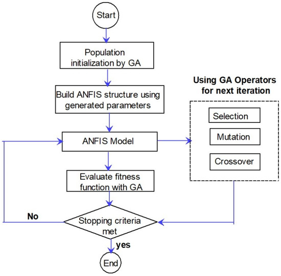
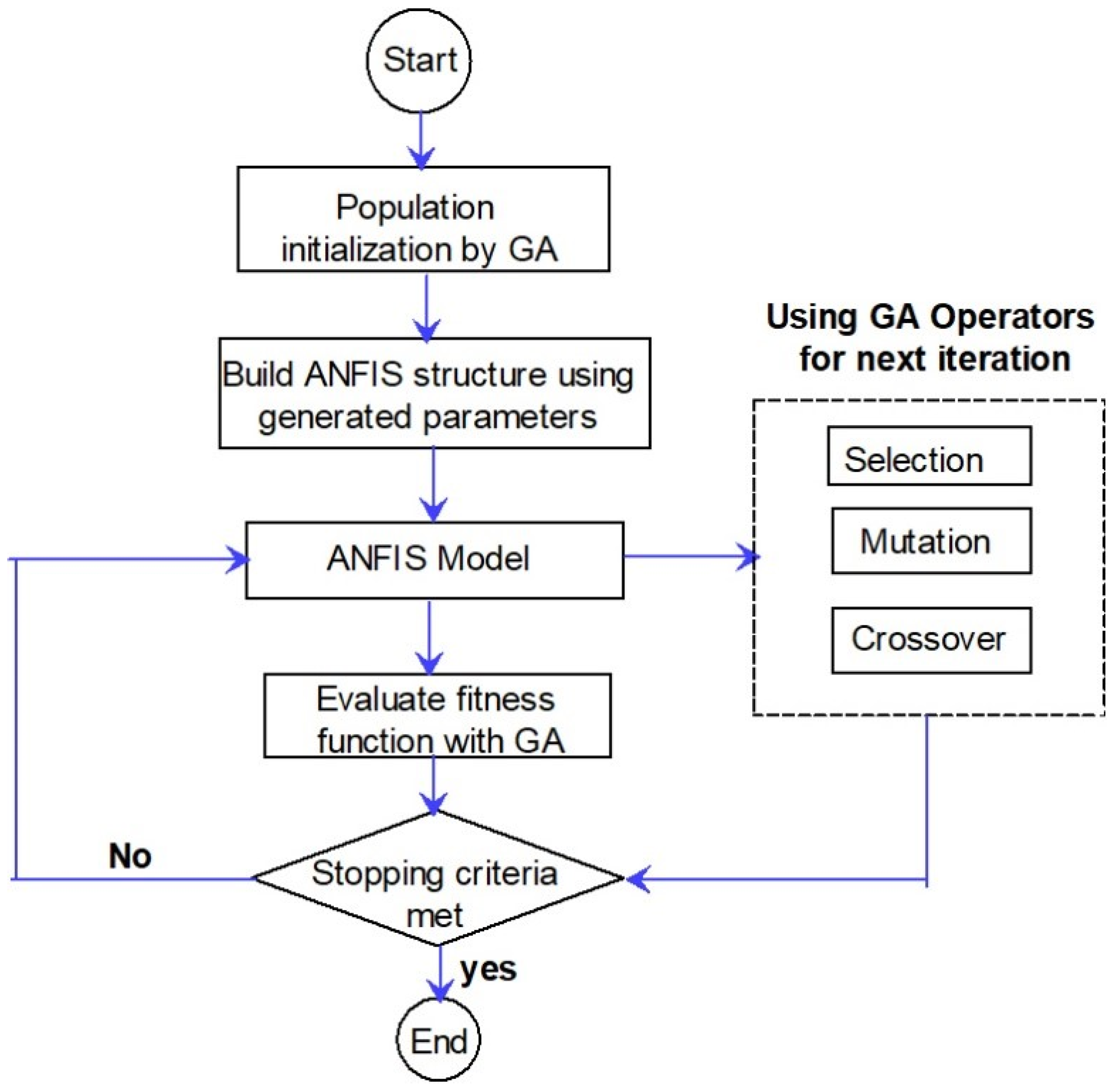
The hybrid ANFIS-GA model integrates the learning capabilities of ANFIS with the global optimization power of GAs. The GA optimizes the structure and parameters of the ANFIS by simulating evolutionary selection and mutation. The ANFIS parameters (shape, centre, and spread of membership function, weights in the neural network structure, fuzzy rules) are encoded into a genetic representation as genes in a chromosome. The fitness of each chromosome is evaluated using the ANFIS prediction accuracy, which is RMSE for this study. The GA selects the best-performing solutions and evolves them over iterations (crossover and mutation). The best set of parameters is used for ANFIS training and the best-trained ANFIS model is used for prediction. Figure 10 illustrates the ANFIS-GA.
Figure 10.
Flowchart of ANFIS-GA.
3.2. Dataset
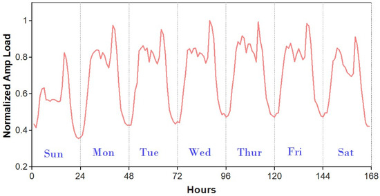
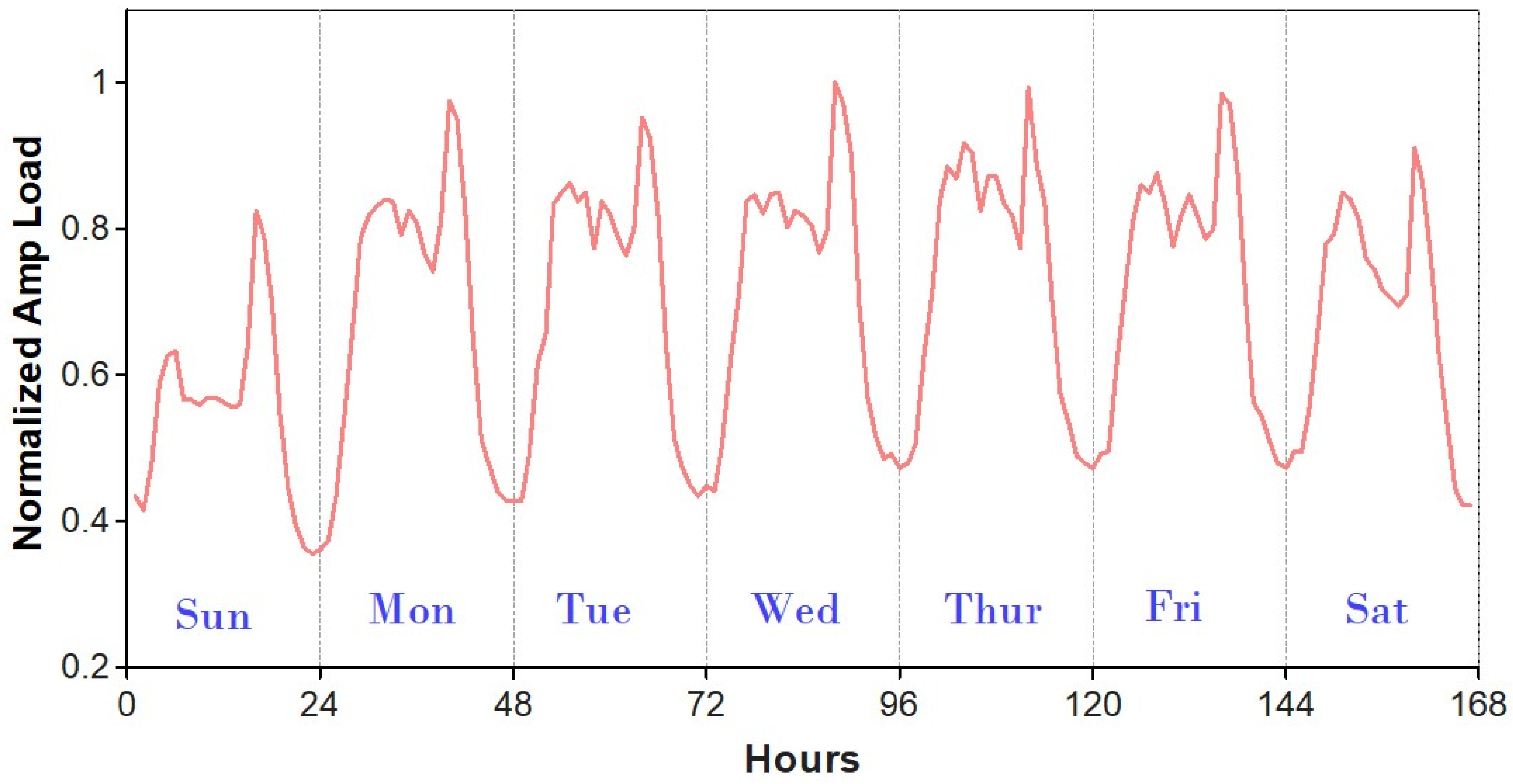
The actual historical load data covering the period of January 2023 to June 2024, comprising hourly electrical Amp load, was obtained from the Rivatex substation in Kenya. The data was recorded from a 45 MVA transformer operating at distribution voltage of 33 KV/11 KV. The Amp load was measured at the circuit breakers (CBs) connecting the transformer to different load feeders. The CBs were rated at 80% of the total load. The weather data, consisting of temperature, wind speed, and humidity were obtained from a Moi University weather station, within the neighbourhood of the Rivatex substation. Figure 11 depicts the normalized hourly Amp-load profile spanning one week (168 hourly loads) as recorded at the Rivatex power utility substation. To capture the complex features of the load profile, the Amp load values from the previous week’s hourly loads were used alongside the weather data as input to the model.
Figure 11.
Normalized hourly aggregated demand profile for one week (December 2023).
3.3. Data Processing
Data pre-processing was performed on the raw dataset to remove distorted data and unwanted variabilities that are not related to the feature variables, such as a sudden drop of load resulting from a change in large industrial or commercial load in the grid. The initial step was to clean the data by correcting erroneous data, removing duplicate entries and addressing missing values. The missing values were handled through imputation, while outliers were removed using a z-score method in MATLAB 2017a. This method is preferable when compared with simple statistical rules (e.g., mean filtering or interquartile range) or regression-based methods because it is simple, scale-independent and adapts better to varying load levels. Thus, it prevents possible the misclassification of peak-hour loads as outliers to preserve the underlying load demand pattern. The noise in the historical data was reduced using moving average smoothing. The data was then normalized by mean centering and variance scaling in order to ensure consistent predictions and avoid the disproportionate influence of various features. The pre-processed dataset contained 12,000 datapoints that were divided into a training part (75%), and a testing and validation part (25%). Note that owing to very high number of datapoints and the narrow interval, plotting the data before cleaning and smoothing is not feasible as the plots generated from raw data are excessively dense and visually cluttered.
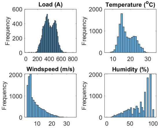
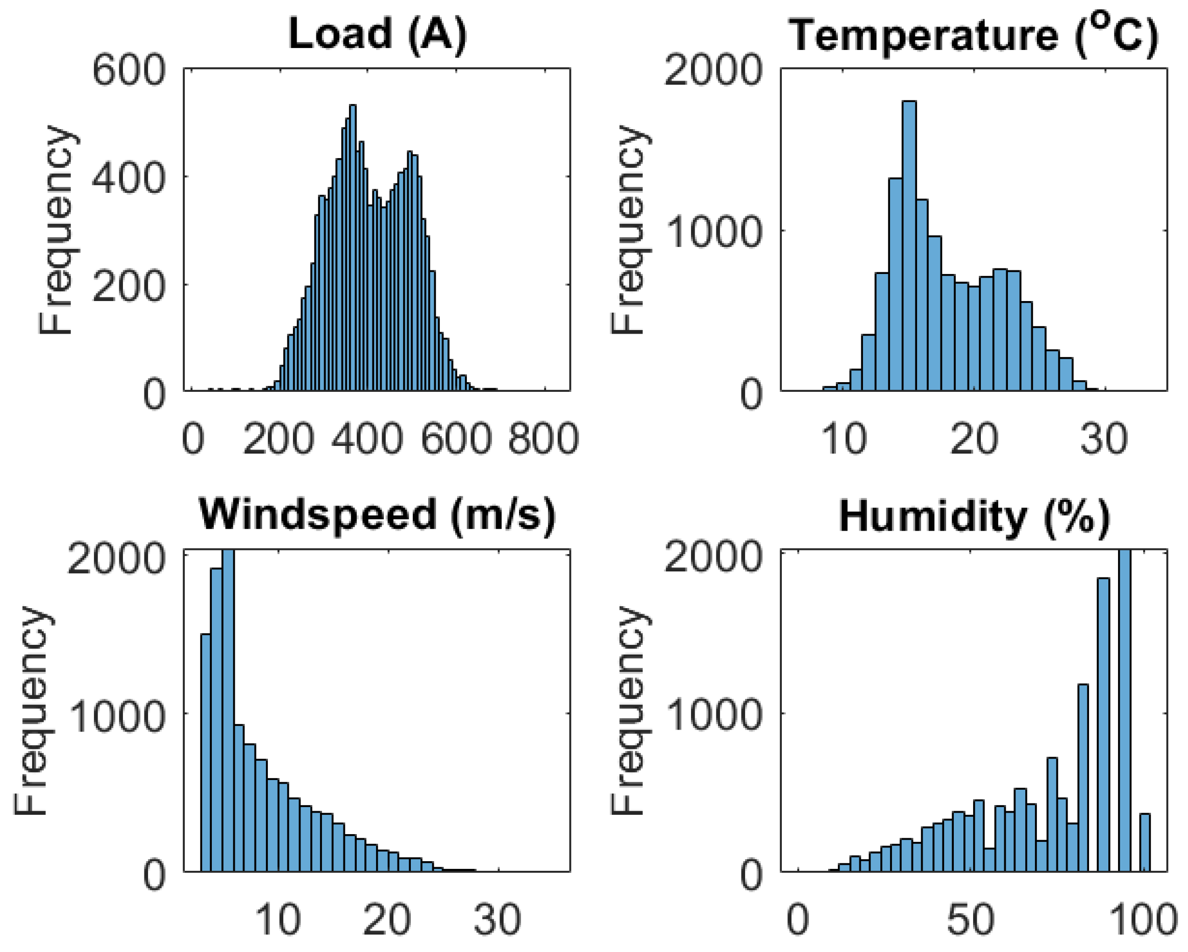
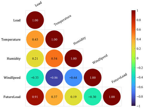
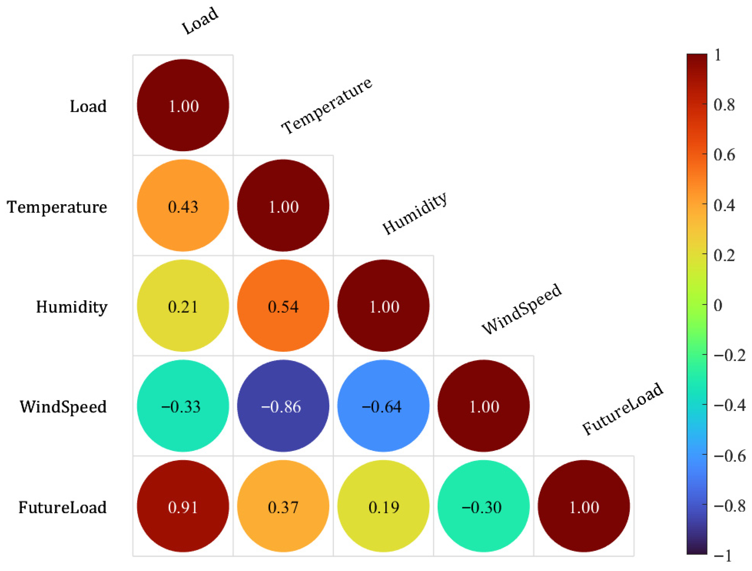
Figure 12 shows the statistical distribution of the data, while Figure 13 shows the correlation analysis results between the Amp load and weather variables. The dependent variable is the Amp load, and the independent variables are the weather parameters. The colour bars in the right of each figure represent the range of the correlation coefficient, and the numbers in the figure represent the correlation coefficient. Among the weather variables, air temperature has the most significant impact on the Amp load with a correlation of 0.43.
Figure 12.
Statistical distribution of the data.
Figure 13.
Correlation heat map of the variables.
3.4. Summary of Hyperparameters
The hybrid models were implemented in MATLAB, with custom optimization routines. The simulations were conducted on a Windows-based workstation using an Intel Corei7 CPU with 16 GB RAM. The key hyperparameters are summarily presented in Table 1.
Table 1.
Summary of the hyperparameters.
4. Results
This study explored different hybridizations of machine learning models and evaluated their comparative prediction performances. The models were hybridized to assess the effectiveness of combining different machine learning algorithms to improve accuracy and reliability in predicting Amp-load behaviour over short time horizons. The results of the study are presented in this section. The Amp-load data was recorded at a one-hour resolution.
4.1. Model Training and Testing
A fitness function (objective function) was employed for the training and testing of the proposed hybrid models. Three frequently used metrics described by Equations (7)–(9), namely the mean absolute percentage error (MAPE), root mean square error (RMSE) and coefficient of determination (R2) were utilized to evaluate the performance of the models.
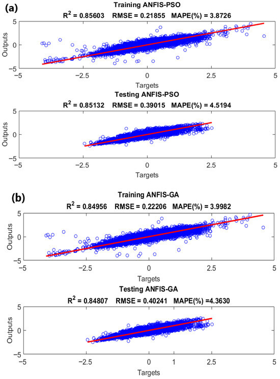
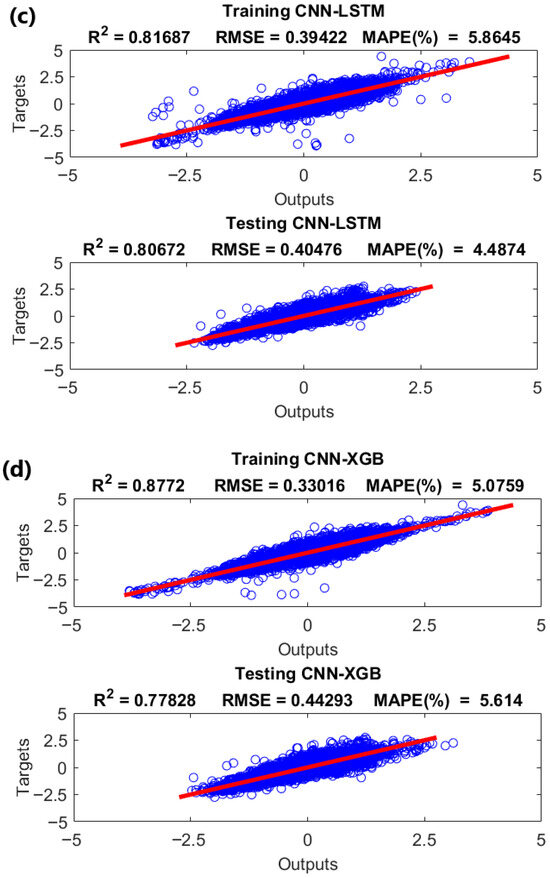
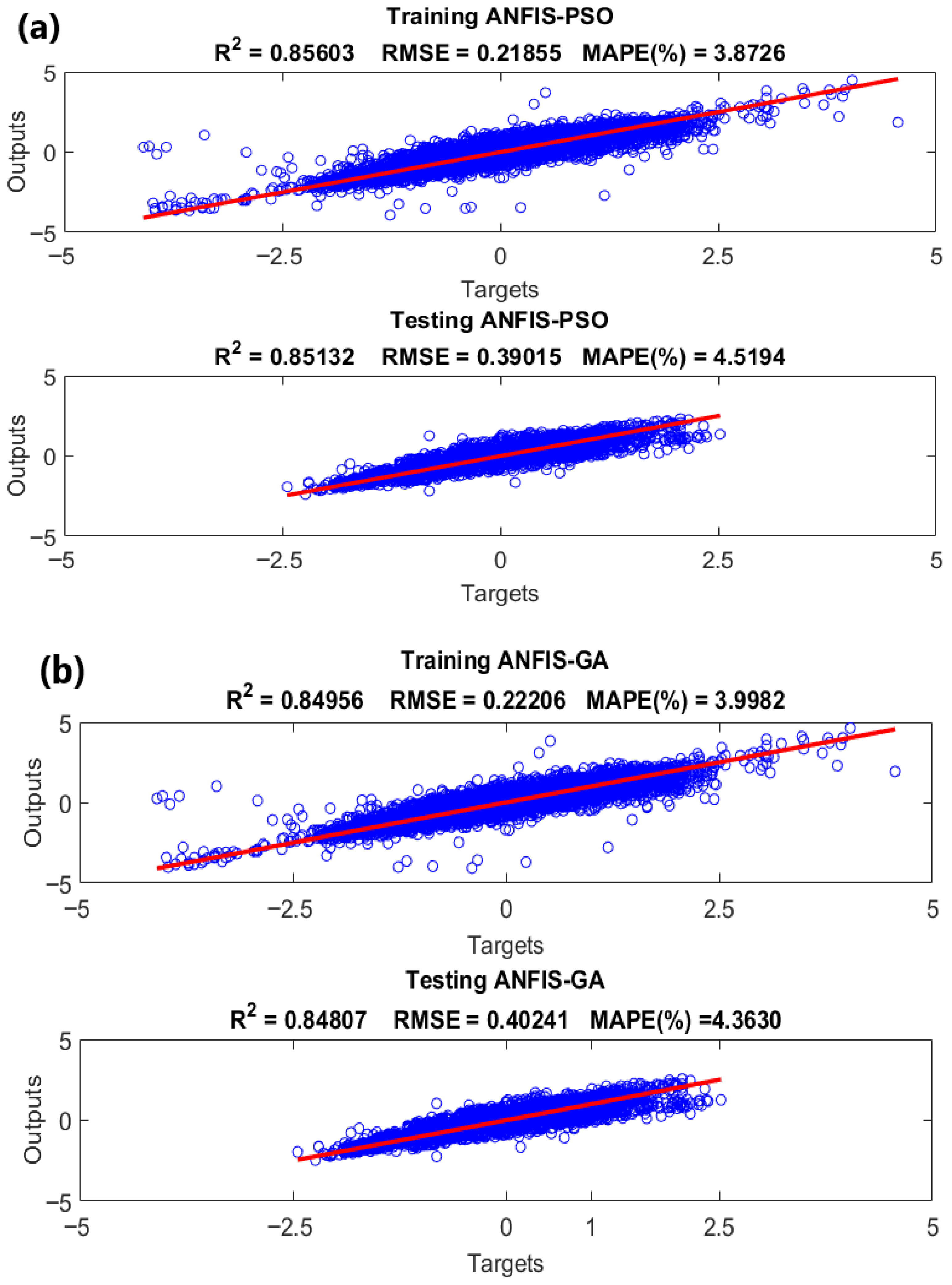
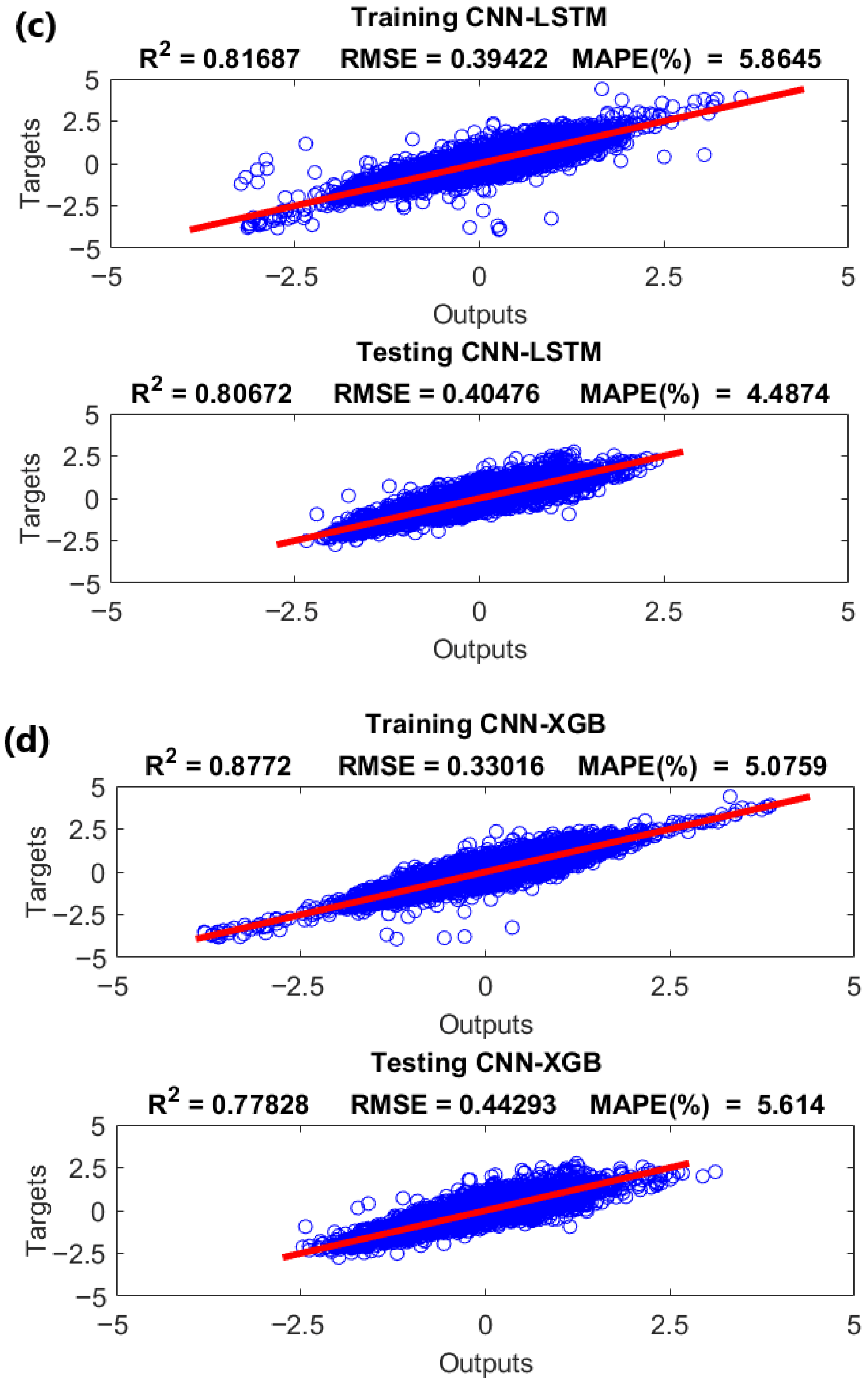
Presented in Figure 14a–d are the outcomes of model training and testing for the four hybrid models considered, i.e., ANFIS-PSO, ANFIS-GA, CNN-LSTM, and CNN-XGB.
Figure 14.
Results of the model training and testing: (a) training and testing of the ANFIS-PSO model; (b) training and testing of the ANFIS-GA model; (c) training and testing of the CNN-LSTM model; (d) training and testing of the CNN-XGB model.
4.2. Model Training and Testing with Load Data Decomposition
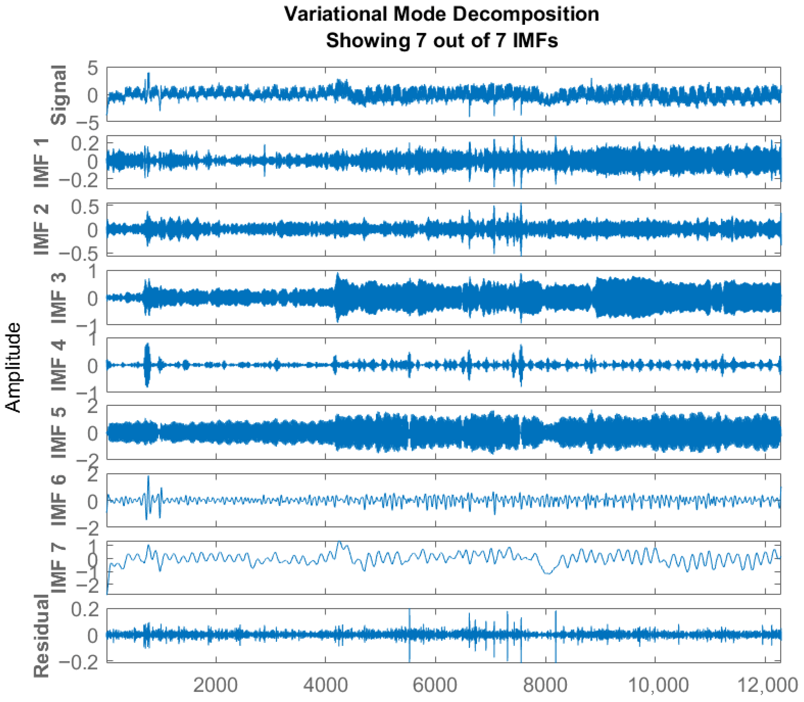
To improve the accuracy of prediction, the Amp-load data was pre-processed using the variational mode decomposition (VMD) technique. The raw Amp-load signal was broken down into sub-signals called Intrinsic Mode Functions (IMF) with distinct spectral characteristics to extract intrinsic features related to Amp-load pattern. This enables better analysis of the load data by reducing the uncertainty and irregularity in the load data. Details of VMD can be reviewed in the work by Ahajjam et al. [35]. The influential parameters, mode number and the penalty factor need to be determined in advance. The default value of the penalty factor, α = 2000, is used in this paper. The data was decomposed into 7 IMFs as shown in Figure 15. The optimal number of modes was determined by k-means clustering of the data. In determining the number of modes, it is noteworthy that a high number of modes may result in mode mixing or purely noisy modes, whereas a low number of modes may lead to duplicate modes [36]. Highly correlated IMFs were grouped and recombined into representative sub-signals to avoid multicollinearity. The reconstructed signal (formed from clustered IMFs) was then used as the input load feature for the hybrid models.
Figure 15.
Variational mode decomposition (VMD) of load signal.
All the CNN hybridized models incurred a shorter training time of between 1 and 2 min compared to the ANFIS hybridized models that incurred a relatively longer training time of between 4 min and 4 min 26 s.
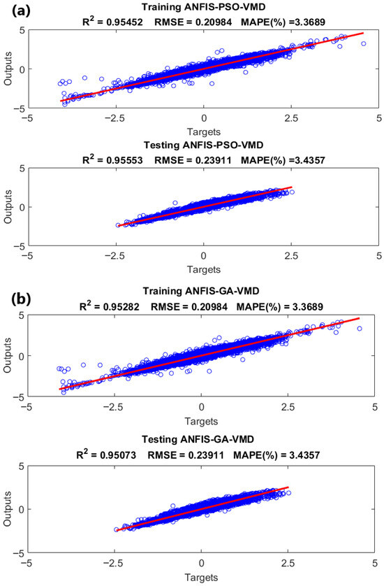
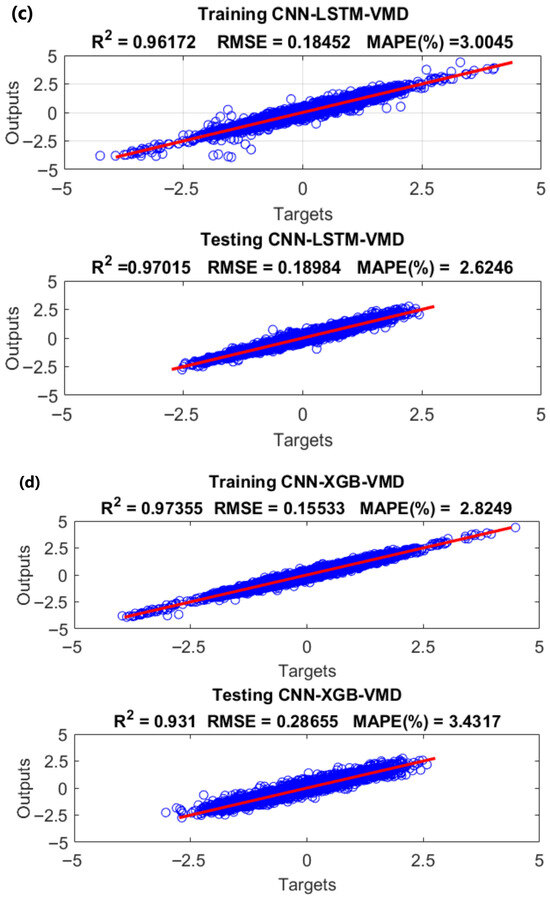
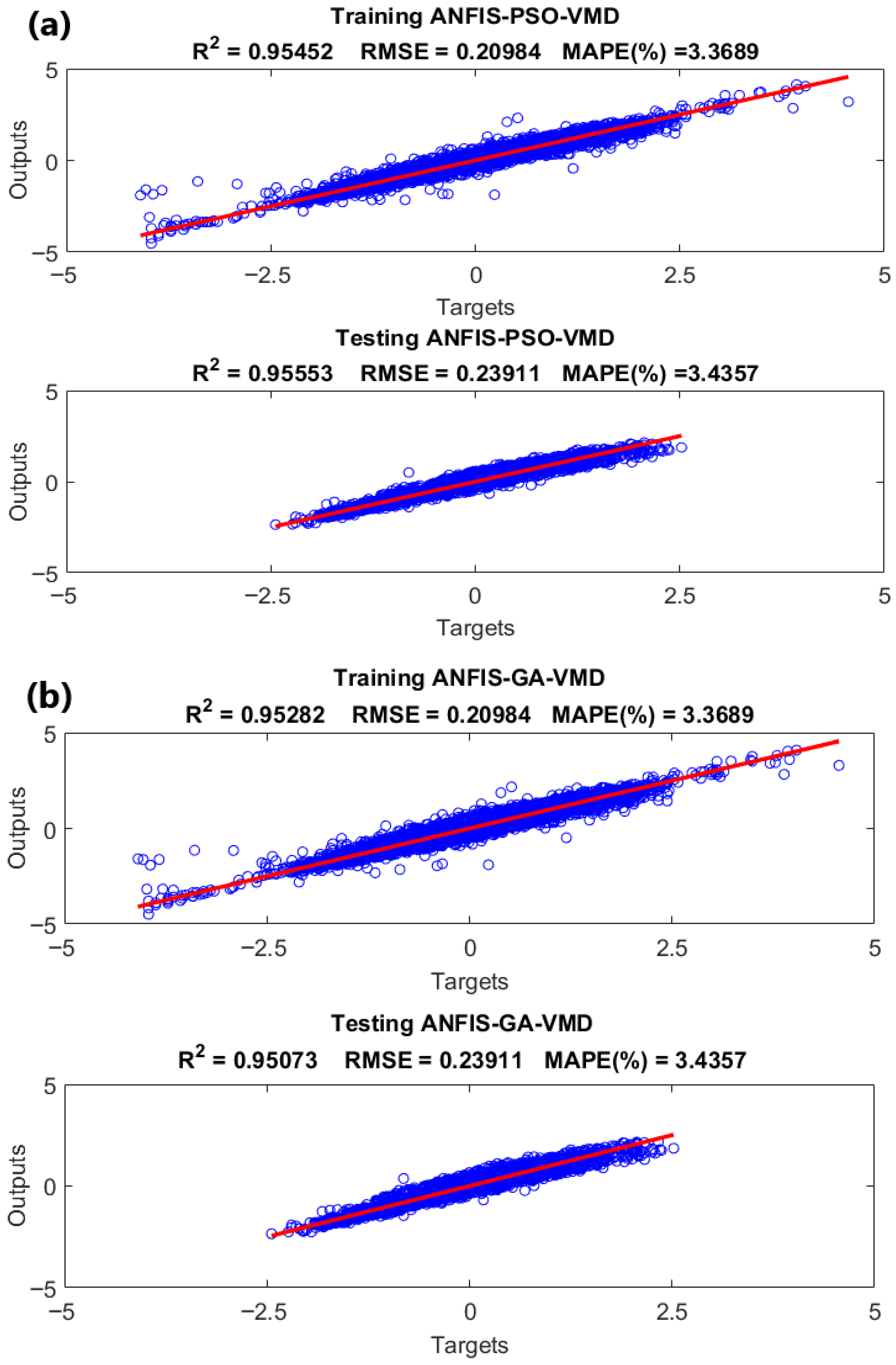
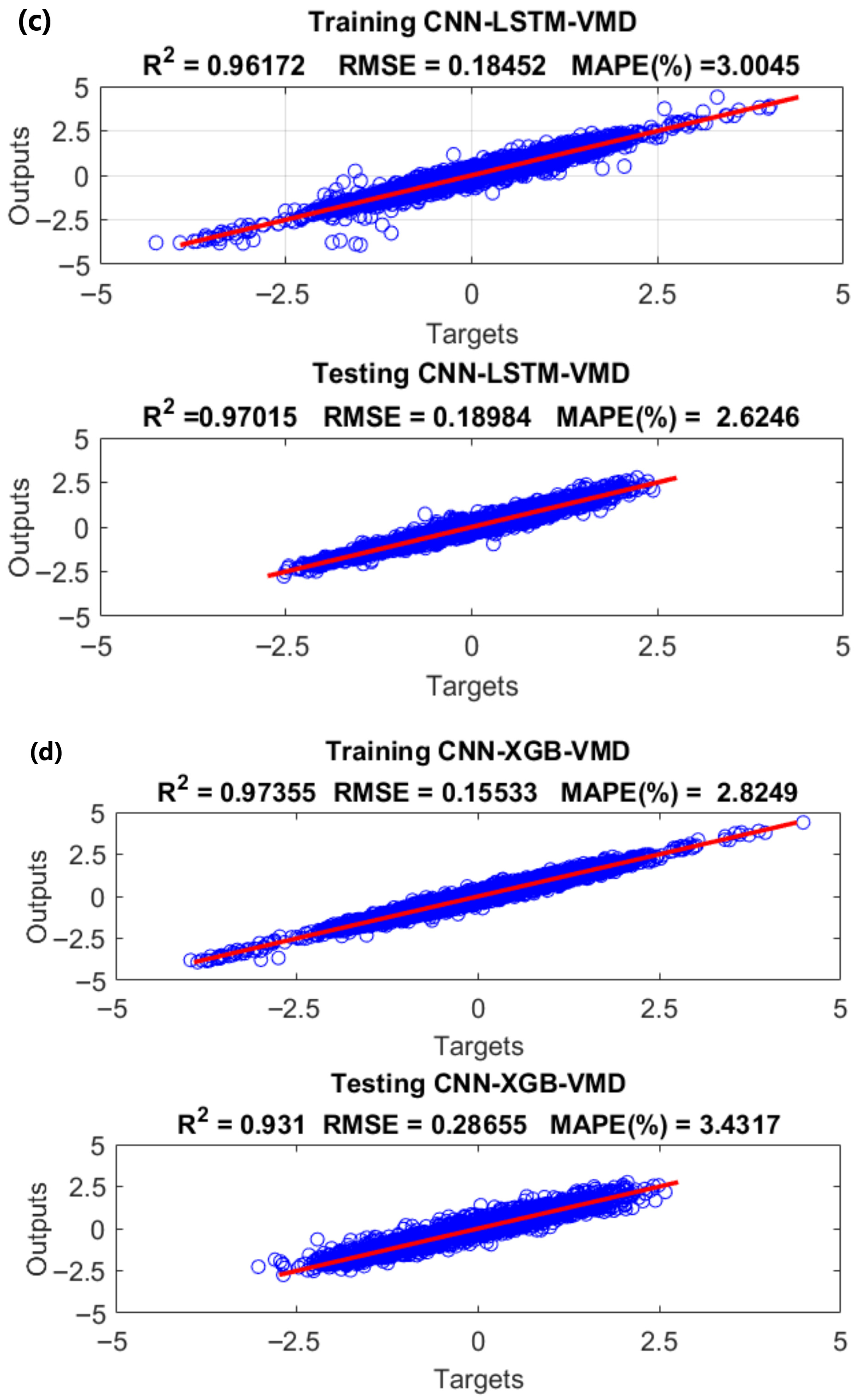
Presented in Figure 16a–d are the results of model training and testing with variable mode decomposition of the load data for the four hybrid models considered, i.e., ANFIS-PSO, ANFIS-GA, CNN-LSTM, and CNN-XGB.
Figure 16.
Results of the model training and testing with load data decomposition: (a) training and testing of the ANFIS-PSO-VMD model; (b) training and testing of the ANFIS-GA-VMD model; (c) training and testing of the CNN-LSTM-VMD model; (d) training and testing of the CNN-XGB-VMD model.
5. Discussions
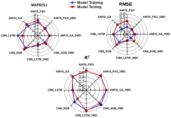
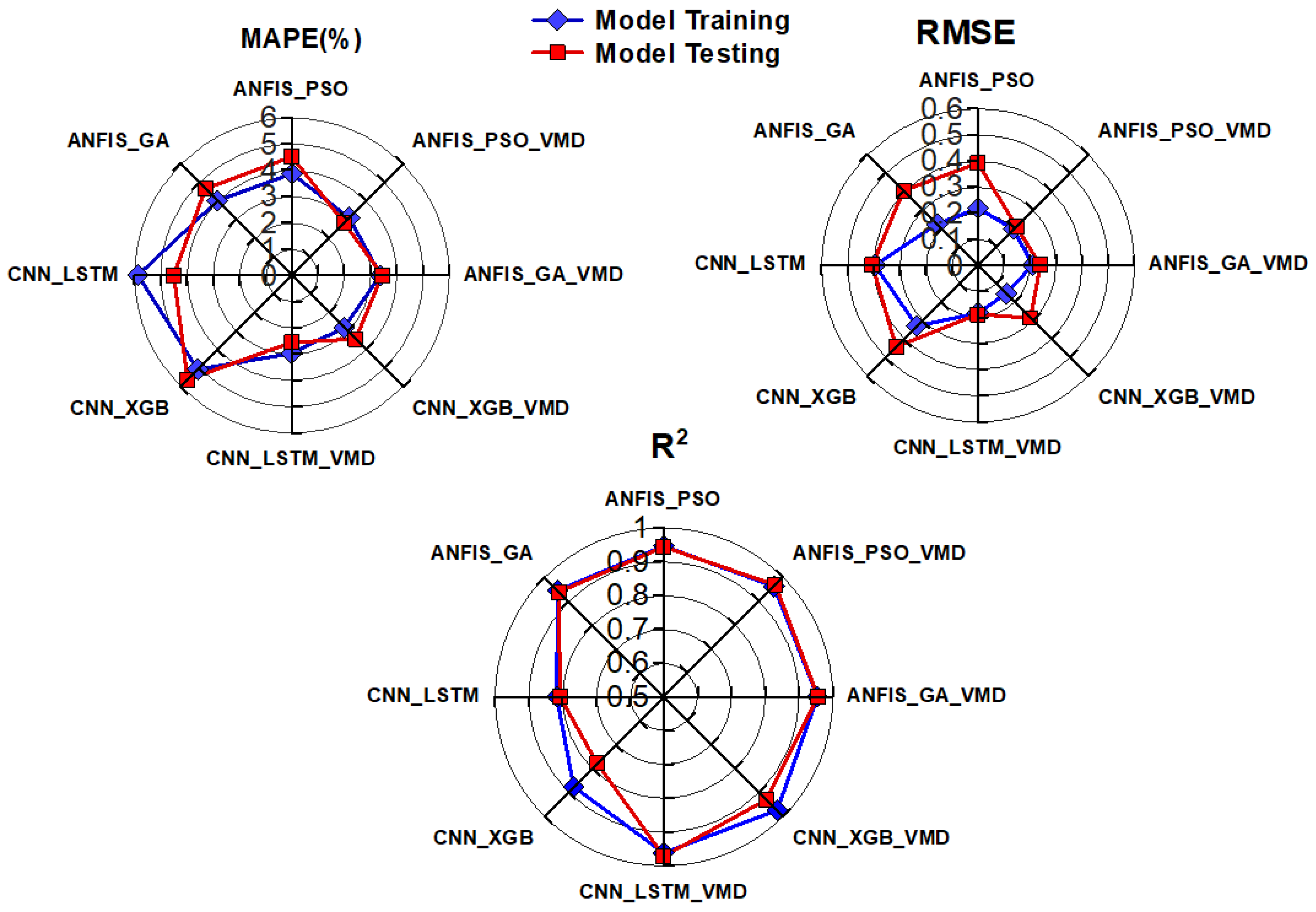
The predictive performance of the four hybrid models was analyzed using three key metrics, namely the MAPE, RMSE and R2. The results are compared using radar plots as shown by Figure 17. The models with a lower MAPE and RMSE and a higher R2 on the testing data perform better. From Figure 17, it is noticeable that hybrid models with variational mode decomposition (VMD) are highly effective for STLP, achieving relatively low MAPEs and RMSEs, with high R2 scores. Overall, two hybrid models, CNN-LSTM-VMD and ANFIS-PSO-VMD, outperformed the other models in all metrics.
Figure 17.
Radar plots of the performance metrics for the hybrid models assessed.
For the models tested without data decomposition, ANFIS-GA and ANFIS-PSO achieve slightly lower MAPEs and RMSEs, and higher R2s, suggesting better predictive accuracy than the CNN-LSTM and CNN-XGB models. Nonetheless, it is noteworthy that models based on evolutional optimization (PSO, GA) show competitive results when properly tuned [24,28]. The ANFIS can capture fuzzy rules and learn them adaptively, enabling accurate approximation of nonlinear relationships, and when optimized with GA or PSO, it can fine-tune rule sets and membership functions efficiently [25].
For the deep-learning models, CNN-LSTM outperformed CNN-XGB in terms of MAPE and RMSE, indicating marginally lower error magnitude on average and better handling of peak loads. The relatively inferior performance by CNN-XGB is attributed to the design of the CNN that is optimized for spatial data and is not efficient for capturing temporal patterns observed in electric load behaviour.
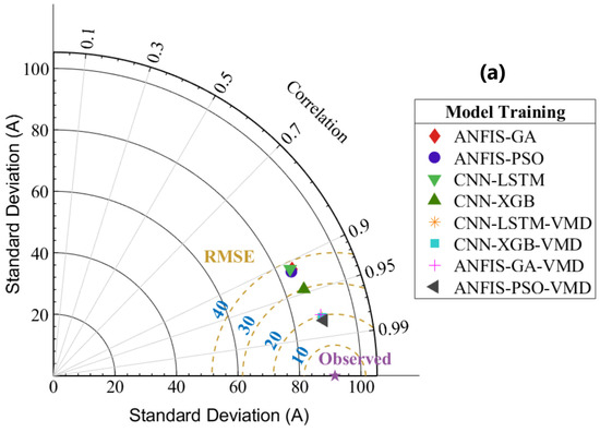
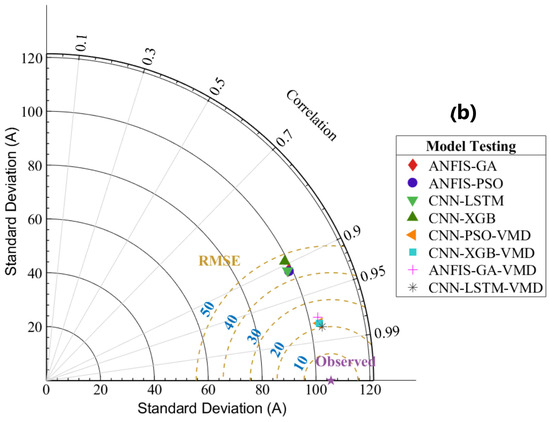
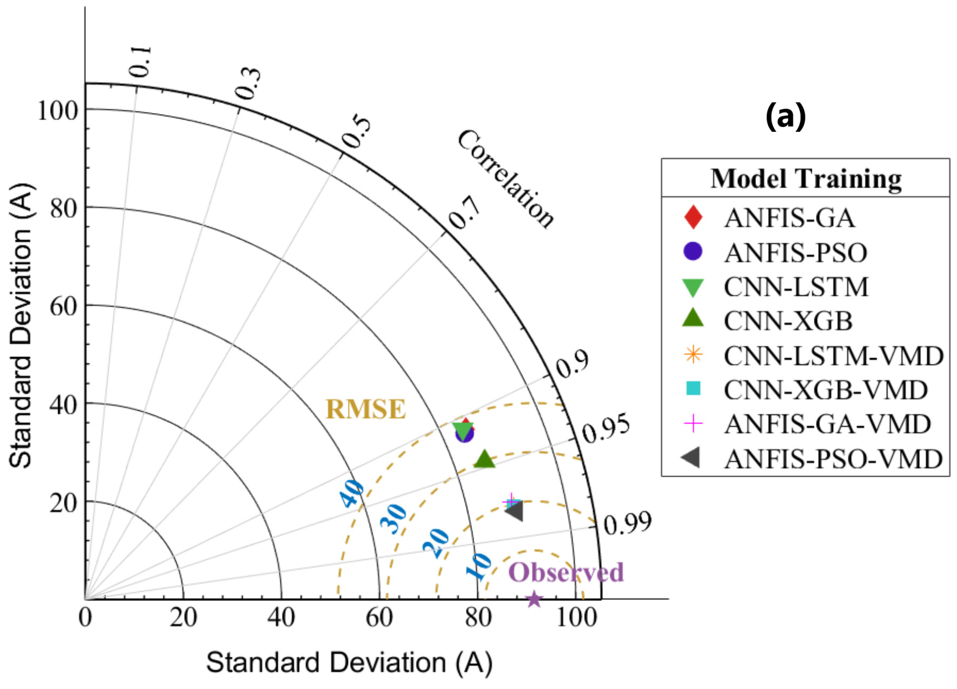
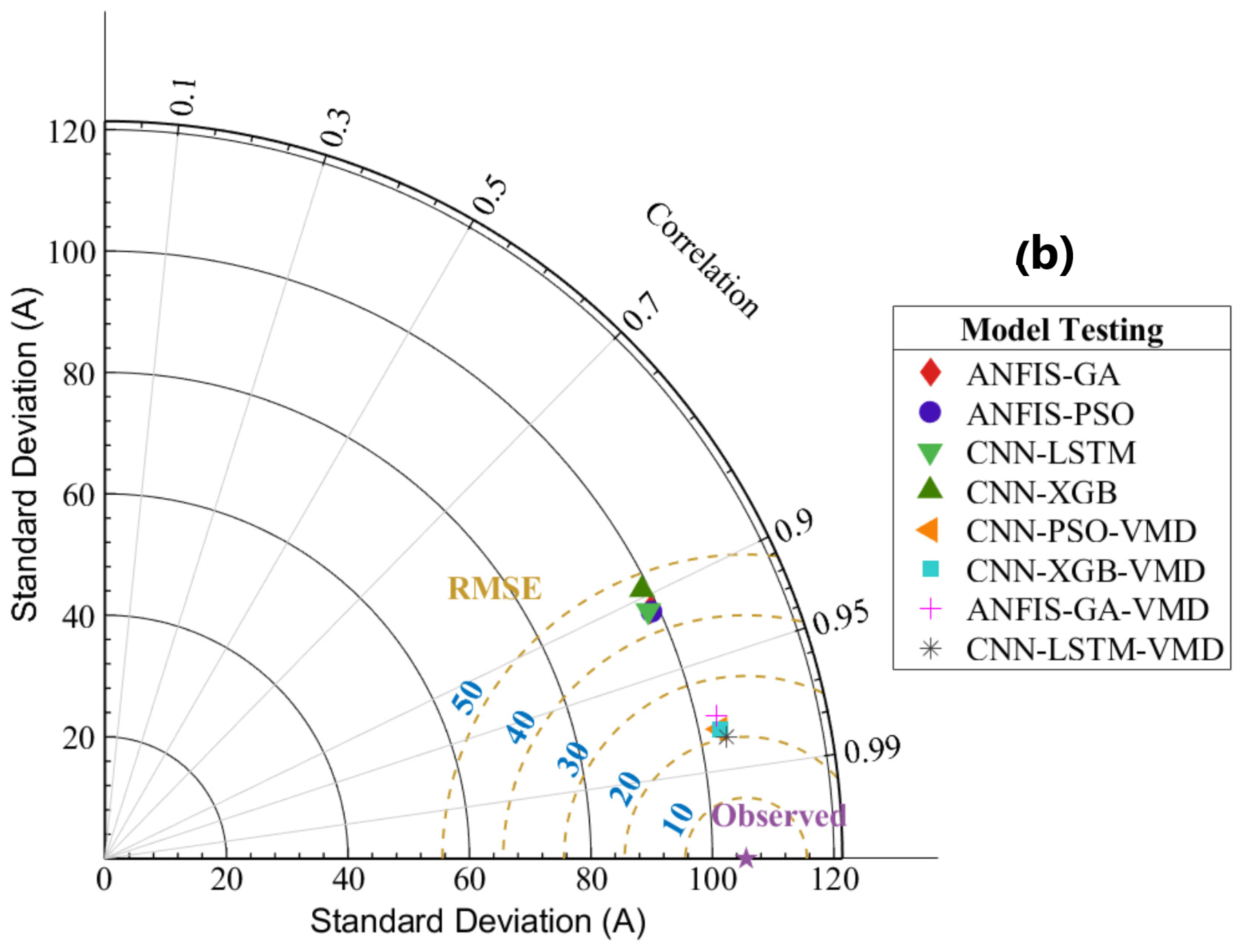
The quality of the predictions by the hybrid models presented here was further compared using the Taylor plots as shown in Figure 18, based on the actual Amp-load signal and not standardized scores. These plots enable direct visual assessment of how closely each hybrid model matches the observed load in terms of amplitude (standard deviation), pattern similarity (correlation) and centred root mean square error. They are particularly appropriate for comparing machine learning models, where pre-processing techniques such as data decomposition or feature extraction may change the variance characteristics of the predicted model. The balance between standard deviation (radial distance), correlation and RMSE determines overall model quality [37]. The observed data represents the reference point with standard deviation equal to that of the observations. If the model point lies farther from the origin than the reference point, it has a larger standard deviation than the observations, and if it lies closer, it has lesser variability than the observations. However, a significantly lower standard deviation would indicate an over-smoothing effect, which may lead to the loss of critical patterns in the load signal, such as peak loads. The angle from the x-axis represents the correlation coefficient. The smaller the angle (model point is closer to the x-axis), the higher the correlation with the observations. Hence, a point that lies directly on the x-axis has a correlation coefficient of 1. The centred root mean square error (RMSE) is represented by the Euclidean distance of the model point from the reference point. A smaller distance corresponds to a smaller RMSE.
Figure 18.
Taylor plots of (a) training data and (b) testing data.
From the results displayed by Figure 18a,b, models trained and tested with data decomposition (VMD) lie closer to the reference point, with a correlation coefficient closer to unity, which demonstrates their superior predictive performance. The results corroborate our initial findings whereby hybrid models demonstrated better performance than convolutional deep learning hybrid models in short-term load prediction. But variational mode decomposition of the load data improved the prediction accuracy across all models.
6. Conclusions
This paper presents a comparative assessment of the prediction performance of hybridized machine learning (ML) models comprising convolutional neural networks with long short-term memory networks and gradient boosting ensembles, and a fuzzy inference system with evolutionary optimization, for short-term Amp-load prediction in medium-voltage electric networks. Based on three statistical indicators, namely MAPE (for accuracy), RMSE (for error minimization) and R2 (for predictive power), and without data decomposition, the adaptive neuro-fuzzy hybrid models with evolutionary optimization (ANFIS-PSO, ANFIS-GA) achieved better performance against CNN-based models. The performance metrics were further evaluated using Taylor plots, which corroborated these findings. The relatively inferior performance by the convolutional neural network hybrid models (CNN-LSTM, CNN-XGB) is attributed to the design of a CNN that is not optimized to model time dependencies, but spatial data. The feature representation in the CNN occuring through convolving learnable filters (kernels) is not efficient for capturing temporal patterns observed in electric load behaviour. The results indicate that if tuned well, hybrid models based on an adaptive neuro-fuzzy approach and optimized with evolutionary algorithms are well suited for short-term load prediction in medium-voltage electric networks given the temporal pattern of the Amp-load behaviour.
Lastly, the pre-processing of the load data by variational mode decomposition (VMD) improved the prediction accuracy of all the models, owing to enhanced feature extraction. When VMD pre-processing was applied, CNN-LSTM-VMD and ANFIS-PSO-VMD outperformed the other models in all metrics. Overall, CNN-LSTM-VMD achieved the best performance, marginally surpassing ANFIS-PSO-VMD.
It is noteworthy that the generalizability of our findings is limited by the single-substation dataset. The future work will extend to multi-substation and network-wide forecasting.
Author Contributions
Conceptualization, Project administration, Formal analysis, Investigation, Writing—original draft (A.B.M.); Data curation, Investigation, Formal analysis, Validation, Software (A.A.); Formal analysis, Writing—review and editing, Visualization (S.S.). All authors have read and agreed to the published version of the manuscript.
Funding
This research received no external funding.
Institutional Review Board Statement
Not applicable.
Informed Consent Statement
Not applicable.
Data Availability Statement
The original contributions presented in this study are included in the article. Further inquiries can be directed to the corresponding author.
Acknowledgments
This study received support from the Norwegian University of Life Sciences (NMBU), Norway, for data analysis under the Norwegian Partnership Programme for Global Academic Cooperation (NORPART).
Conflicts of Interest
Author Abraham Arusei was employed by the company Kenya Power & Lighting Company Ltd. The remaining authors declare that the research was conducted in the absence of any commercial or financial relationships that could be construed as a potential conflict of interest.
Abbreviations
The following abbreviations are used in this manuscript:
| VMD | Variational Mode Decomposition |
| STLP | Short-Term Load Prediction |
| CNN | Convolutional Neural Networks |
| LSTM | Long Short-Term Memory |
| XGB | Extreme Gradient Boosting |
| ML | Machine Learning |
| PSO | Particle Swarm Optimization |
| GA | Genetic Algorithms |
| ANFIS | Adaptive Neuro-Fuzzy Inference System |
| MV | Medium Voltage |
| MAPE | Mean Absolute Percent Error |
| RMSE | Root Mean Square Error |
| IMF | Intrinsic Mode Functions |
| RNN | Recurrent Neural Networks |
References
- Kuster, B.; Rezgui, Y.; Mourshed, M. Electrical load forecasting models: A critical systematic review. Sustain. Cities Soc. 2017, 35, 257–270. [Google Scholar] [CrossRef] [Scilit]
- Shohan, M.J.A.; Faruque, M.O.; Foo, S.Y. Forecasting of electric load using a hybrid LSTM–Neural Prophet model. Energies 2022, 15, 2158. [Google Scholar] [CrossRef] [Scilit]
- Mir, A.A.; Alghassab, M.; Ullah, K.; Khan, Z.A.; Lu, Y.; Imran, M. A review of electricity demand forecasting in low- and middle-income countries: The demand determinants and horizons. Sustainability 2020, 12, 5931. [Google Scholar] [CrossRef] [Scilit]
- Steinbuks, J. Assessing the accuracy of electricity production forecasts in developing countries. Int. J. Forecast. 2019, 35, 1175–1185. [Google Scholar] [CrossRef] [Scilit]
- Indrawati, A.; Girsang, A.S. Electricity demand forecasting using adaptive neuro-fuzzy inference system and particle swarm optimization. Int. Rev. Autom. Control 2016, 9, 397–404. [Google Scholar] [CrossRef] [Scilit]
- Patel, H.; Pandya, M.; Aware, M. Short term load forecasting of Indian system using linear regression and artificial neural network. In Proceedings of the 5th Nirma University International Conference on Engineering, Ahmedabad, India, 26–28 November 2015. [Google Scholar]
- Lynn, T.E. Short-Term Electrical Load Forecasting for an Institutional/Industrial Power System Using an Artificial Neural Network. Master’s Thesis, University of Tennessee, Knoxville, TN, USA, 2013. [Google Scholar]
- Phuangpornpitak, N.; Prommee, W. A study of load demand forecasting models in electric power system operation and planning. GMSARN Int. J. 2016, 10, 19–24. [Google Scholar]
- Yazici, I.; Beyca, O.F.; Delen, D. Deep-learning-based short-term electricity load forecasting: A real case application. Eng. Appl. Artif. Intell. 2022, 109, 104645. [Google Scholar] [CrossRef] [Scilit]
- Rodríguez, F.; Martín, F.; Fontán, L.; Galarza, A. Very short-term load forecaster based on a neural network technique for smart grid control. Energies 2020, 13, 5210. [Google Scholar] [CrossRef] [Scilit]
- Houimli, R.; Zmami, M.; Ben-Salha, O. Short-term electric load forecasting in Tunisia using artificial neural networks. Energy Syst. 2020, 11, 357–375. [Google Scholar] [CrossRef] [Scilit]
- Khan, A.R.; Razzaq, S.; Alquthami, T.; Moghal, M.R.; Amin, A.; Mahmood, A. Day-ahead load forecasting for IESCO using artificial neural network and bagged regression tree. In Proceedings of the 1st International Conference on Power, Energy and Smart Grid (ICPESG), Mirpur, Azad Kashmir, Pakistan, 9–10 April 2018; pp. 1–6. [Google Scholar] [CrossRef] [Scilit]
- Li, W.Q.; Chang, L. A combination model with variable weight optimization for short-term electrical load forecasting. Energy 2018, 164, 575–593. [Google Scholar] [CrossRef] [Scilit]
- Shi, J. Load forecasting for regional integrated energy systems based on complementary ensemble empirical mode decomposition and multi-model fusion. Appl. Energy 2024, 353, 122146. [Google Scholar] [CrossRef] [Scilit]
- Massaoudi, M.; Refaat, S.S.; Chihi, I.; Trabelsi, M.; Oueslati, F.S.; Abu-Rub, H. A novel stacked generalization ensemble-based hybrid LGBM–XGB–MLP model for short-term load forecasting. Energy 2021, 214, 118874. [Google Scholar] [CrossRef] [Scilit]
- Ospina, J.; Newaz, A.; Faruque, M.O. Forecasting of PV plant output using a hybrid wavelet-based LSTM–DNN model. IET Renew. Power Gener. 2019, 13, 1087–1095. [Google Scholar] [CrossRef] [Scilit]
- Haq, M.R.; Ni, Z. A new hybrid model for short-term electricity load forecasting. IEEE Access 2019, 7, 125413–125423. [Google Scholar] [CrossRef] [Scilit]
- Zhang, J.; Wei, Y.M.; Li, D.; Tan, Z.; Zhou, J. Short-term electricity load forecasting using a hybrid model. Energy 2018, 158, 774–781. [Google Scholar] [CrossRef] [Scilit]
- Xu, L.; Li, C.; Xie, X.; Zhang, G. Long short-term memory network-based hybrid model for short-term electrical load forecasting. Information 2018, 9, 165. [Google Scholar] [CrossRef] [Scilit]
- Olagoke, M.D.; Ayeni, A.; Hambali, M.A. Short-term electric load forecasting using neural network and genetic algorithm. Int. J. Appl. Inf. Syst. 2016, 10, 22–28. [Google Scholar] [CrossRef] [Scilit]
- Tudose, A.M.; Picioroaga, I.I.; Sidea, D.O.; Bulac, C.; Boicea, V.A. Short-term load forecasting using convolutional neural networks in COVID-19 context: The Romanian case study. Energies 2021, 14, 4046. [Google Scholar] [CrossRef] [Scilit]
- Muzaffar, S.; Afshari, A. Short-term load forecasts using LSTM networks. Energy Procedia 2019, 158, 2922–2927. [Google Scholar] [CrossRef] [Scilit]
- Guo, X.; Zhao, Q.; Wang, S.; Shan, D.; Gong, W. A short-term load forecasting model of LSTM neural network considering demand response. Complexity 2021, 2021, 598267. [Google Scholar] [CrossRef] [Scilit]
- Robati, F.N.; Iranmanesh, S. Inflation rate modeling: Adaptive neuro-fuzzy inference system and particle swarm optimization approach. MethodsX 2020, 7, 101062. [Google Scholar] [CrossRef] [Scilit] [PubMed]
- Yang, Y.; Chen, Y.; Wang, Y.; Li, C.; Li, L. Modelling a combined method based on ANFIS and neural network improved by differential evolution algorithm for short-term electricity demand forecasting. Appl. Soft Comput. 2016, 49, 663–675. [Google Scholar] [CrossRef] [Scilit]
- Sagias, V.D.; Zacharia, P.; Tempeloudis, A.; Stergiou, C. Adaptive neuro-fuzzy inference system-based predictive modeling of mechanical properties in additive manufacturing. Machines 2024, 12, 523. [Google Scholar] [CrossRef] [Scilit]
- Katoch, S.; Chauhan, S.S.; Kumar, V. A review on genetic algorithm: Past, present, and future. Multimed. Tools Appl. 2021, 80, 8091–8126. [Google Scholar] [CrossRef] [Scilit]
- Ray, P.; Panda, S.K.; Mishra, D.P. Short-term load forecasting using genetic algorithm. In Computational Intelligence in Data Mining; Behera, H., Nayak, J., Naik, B., Abraham, A., Eds.; Springer: Singapore, 2019; pp. 863–872. [Google Scholar] [CrossRef] [Scilit]
- Santra, A.S.; Lin, J. Integrating long short-term memory and genetic algorithm for short-term load forecasting. Energies 2019, 12, 2040. [Google Scholar] [CrossRef] [Scilit]
- Ozerdem, O.C.; Ebenezer, O.; Olaniyi, E.O.; Oyedotun, O.K. Short-term load forecasting using particle swarm optimization neural network. Procedia Comput. Sci. 2017, 120, 382–393. [Google Scholar] [CrossRef] [Scilit]
- Chafi, Z.S.; Afrakhte, H. Short-term load forecasting using neural network and particle swarm optimization algorithm. Math. Probl. Eng. 2021, 2021, 598267. [Google Scholar] [CrossRef] [Scilit]
- Hong, Y.-Y.; Chan, Y.-H. Short-term electric load forecasting using particle swarm optimization-based convolutional neural network. Eng. Appl. Artif. Intell. 2023, 126, 106773. [Google Scholar] [CrossRef] [Scilit]
- Omer, Z.M.; Shareef, H. Comparison of decision tree-based ensemble methods for prediction of photovoltaic maximum current. Energy Convers. Manag. X 2022, 16, 100333. [Google Scholar] [CrossRef] [Scilit]
- Ahmed, S.; Raza, B.; Hussain, L.; Aldweesh, A.; Omare, A.; Khan, M.S.; Elding, E.T.; Nadim, M.A. Deep learning ResNet101 and ensemble XGBoost algorithm with hyperparameter optimization for lung cancer prediction. Appl. Artif. Intell. 2023, 37, 2166222. [Google Scholar] [CrossRef] [Scilit]
- Ahajjam, M.A.; Licea, D.B.; Ghogho, M.; Kobbane, A. Experimental investigation of variational mode decomposition and deep learning for short-term multi-horizon residential electric load forecasting. Appl. Energy 2022, 326, 119963. [Google Scholar] [CrossRef] [Scilit]
- Dragomiretskiy, K.; Zosso, D. Variational mode decomposition. IEEE Trans. Signal Process. 2014, 62, 531–544. [Google Scholar] [CrossRef] [Scilit]
- Taylor, K.E. Summarizing multiple aspects of model performance in a single diagram. J. Geophys. Res. 2001, 106, 7183–7192. [Google Scholar] [CrossRef] [Scilit]

Disclaimer/Publisher’s Note: The statements, opinions and data contained in all publications are solely those of the individual author(s) and contributor(s) and not of MDPI and/or the editor(s). MDPI and/or the editor(s) disclaim responsibility for any injury to people or property resulting from any ideas, methods, instructions or products referred to in the content. |
© 2026 by the authors. Licensee MDPI, Basel, Switzerland. This article is an open access article distributed under the terms and conditions of the Creative Commons Attribution (CC BY) license.