MI-Convex Approximation for the Optimal Siting and Sizing of PVs and D-STATCOMs in Distribution Networks to Minimize Investment and Operating Costs

Abstract

The optimal integration of photovoltaic (PV) systems and distribution static synchronous compensators (D-STATCOMs) in electrical distribution networks is important to reduce their operating costs, improve their voltage profiles, and enhance their power quality. To this effect, this paper proposes a mixed-integer convex (MI-Convex) optimization model for the optimal siting and sizing of PV systems and D-STATCOMs, with the aim of minimizing investment and operating costs in electrical distribution networks. The proposed model transforms the traditional mixed-integer nonlinear programming (MINLP) formulation into a convex model through second-order conic relaxation of the nodal voltage product. This model ensures global optimality and computational efficiency, which is not achieved using traditional heuristic-based approaches. The proposed model is validated on IEEE 33- and 69-bus test systems, showing a significant reduction in operating costs in both feeders compared to traditional heuristic-based approaches such as the vortex search algorithm (VSA), the sine-cosine algorithm (SCA), and the sech-tanh optimization algorithm (STOA). According to the results, the MI-convex model achieves cost savings of up to 38.95% in both grids, outperforming the VSA, SCA, and STOA.

1. Introduction

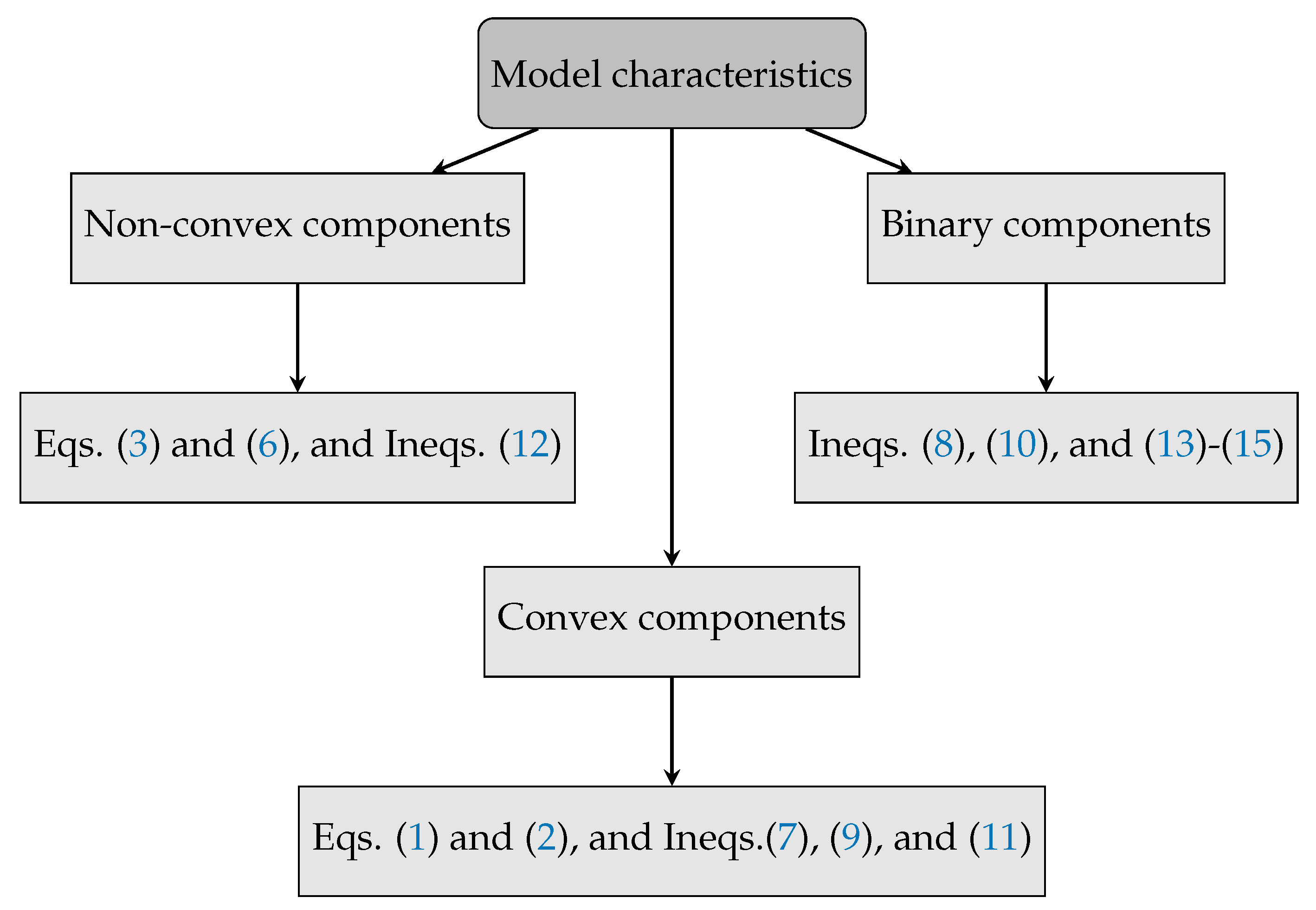
1.1. General Context

The increasing demand for electrical energy and the need to reduce carbon emissions have driven the integration of renewable sources into power systems [1,2,3]. In this context, photovoltaic solar (PV) energy has emerged as a key alternative due to its availability, modularity, and steadily decreasing costs [4,5,6]. However, the large-scale penetration of PV generation introduces new operational challenges in distribution networks, such as voltage fluctuations, increased technical losses, and line congestion [7,8]. To mitigate these effects, renewable generation must be complemented with reactive power compensation technologies, e.g., distribution static synchronous compensators (D-STATCOMs), which help to improve voltage stability and power quality [9,10]. However, implementing these devices requires appropriate planning strategies that balance technical feasibility and economic viability [11].

The integration of these resources poses both technical and economic challenges, as improper placement and sizing can negatively impact power supply quality and system profitability [12,13]. In this context, it is essential to develop optimization methodologies that enable efficient integration while ensuring maximum utilization of the available resources as well as sustainable grid management [14]. The problem regarding the optimal integration of PV generators and D-STATCOMs belongs to the family of mixed-integer nonlinear programming (MINLP) models that simultaneously consider investment, operating, and maintenance costs in addition to the technical constraints of the grid.

1.2. Motivation

In today’s energy landscape, the growing demand for and transition towards more sustainable electrical systems have driven the adoption of distributed renewable sources, particularly PV energy [15,16]. However, the large-scale integration of these resources into traditional distribution networks, originally designed for unidirectional power flow, presents operational challenges such as voltage fluctuations, network element overloads, and increased technical losses [17,18]. In this context, optimizing the placement and sizing of PV generators and reactive power compensation devices becomes a crucial factor in ensuring an efficient and economically viable energy transition, underscoring the integration of PV generators, D-STATCOMs, and other measurement devices into the electrical infrastructure as a vital part of the process.

The implementation of strategies for the integration of PV generators and D-STATCOMs not only improves the efficiency of distribution power systems but also provides economic and environmental benefits. Furthermore, promoting more efficient use of distribution infrastructure encourages the development of distributed generation projects in non-interconnected or isolated areas, fostering rural electrification and reducing dependence on fossil fuels [19,20]. In this regard, this study aims to provide optimization tools that support strategic planning aligned with energy policies and global sustainability commitments.

1.3. Literature Review

The following is an analysis of the main studies published in the last five years in relation to the placement and sizing of PV generators and D-STATCOMs.

In [21], the authors presented a hybrid analytical and metaheuristic optimization methodology for siting and sizing PV generators and D-STATCOMs in distribution networks, aiming to minimize losses and improve voltage profiles. They employed particle swarm optimization (PSO), combined with Monte Carlo simulation, to model probabilistic demand. Validations conducted in a real distribution network in southern Kerman showed improvements in voltage profiles and reductions in active and reactive power losses. However, PSO does not guarantee a global optimum and may suffer from premature convergence. Additionally, while Monte Carlo simulation helps to model demand uncertainty, it increases computational complexity without necessarily enhancing the solution quality.

The authors of [22] proposed an approach based on the rat swarm optimization (RSO) algorithm for the optimal siting and sizing of PV generators and D-STATCOMs in distribution networks, with the purpose of minimizing active power losses, improving voltage profiles, and reducing voltage deviation. The methodology was validated on the IEEE 33-node system, showing reductions in power losses ranging from 210.996 kW to 26.155 kW and an improved minimum voltage of 0.98 p.u. with the simultaneous integration of the aforementioned devices. However, while RSO is a robust metaheuristic technique, it does not guarantee global optimality and can be affected by initialization quality and premature convergence.

The study by [20] presented an approach based on the black widow optimization (BWO) algorithm for the optimal siting and sizing of PV generators and D-STATCOMs in radial distribution networks, whose objective function aimed to minimize power losses and improve voltage profiles. When applied to the IEEE 12-, 33-, and 69-node systems, the method demonstrated significant loss reductions and voltage stability improvements, achieving a reduction of up to 96% in active power losses in some cases. However, while BWO enables the exploration of multiple solutions, it is a metaheuristic technique that does not guarantee global optimality and is sensitive to parameter initialization. Additionally, the study did not explicitly address the investment and operating costs, thereby limiting its applicability in scenarios where economic feasibility is a key factor for distribution network planning.

In [23], the problem regarding the optimal siting and sizing of distributed generators and D-STATCOMs in distribution networks was addressed using the grasshopper optimization algorithm (GOA). In this model, the objective function sought to minimize active power losses and improve the voltage stability index (VSI) of the grid. To validate this method, the IEEE 33-node system was used, achieving an 81.5% reduction in power losses and a 30.7% increase in the VSI when considering multiple DGs and D-STATCOMs. Despite its advantages, however, as a metaheuristic technique, the GOA cannot guarantee convergence to the global optimum. Additionally, this methodology did not incorporate explicit economic constraints in the objective function, which may limit its applicability in scenarios where investment and operating cost optimization is a key factor.

The authors of [24] developed a methodology based on the modified horned lizard optimization algorithm (MHLOA) for the optimal siting and sizing of PV systems and D-STATCOMs in distribution networks while considering uncertainty. The objective function aimed for cost minimization, emissions reduction, voltage deviation mitigation, and active power loss reduction. This approach was validated on the IEEE 33-node system, exhibiting significantly reduced annual costs, power losses, and pollutant emissions. Despite its comprehensive approach, the MHLOA also does not guarantee convergence to the global optimum and may be affected by premature convergence or sensitivity to the initial parameters. Additionally, while this study accounted for uncertainty in load, pricing, and solar irradiance, it did not analyze the problem’s convexity or provide theoretical guarantees of optimality, which may limit the accuracy and reliability of planning in more demanding scenarios.

In [25], the authors proposed a methodology based on the GOA for the optimal reconfiguration of distribution networks in the presence of D-STATCOMs and PV generators. The objective function focused on minimizing power losses and improving voltage profiles in radial distribution networks under different load conditions. This method was validated on the IEEE 33-, 69-, and 118-node systems, achieving significant loss reductions and voltage stability improvements when compared with previous approaches like the modified pollination algorithm and the fuzzy ant colony optimization algorithm. Despite the results obtained, this study primarily dealt with loss reduction and voltage profile improvement without explicitly considering investment and operating cost minimization—a crucial factor in planning distribution networks with distributed energy resources.

The authors of [26] presented an approach based on the modified antlion optimizer (MALO) for the optimal siting and sizing of PV generators and D-STATCOMs in radial distribution networks while also considering network reconfiguration. The objective function focused on minimizing power losses, improving the voltage profile, and reducing the system’s operating costs. This methodology was validated on the IEEE 118-node system and a real 317-node network belonging to BESCOM (India), achieving power loss reductions of 41.47% in the IEEE system and 59.34% in the 317-node network while using a ZIP load model. Although the proposed methodology significantly improves loss reduction and voltage stability, its metaheuristic approach does not ensure global optimality. In scenarios where economic feasibility and theoretical optimality are critical, exact optimization approaches can provide greater reliability and efficiency in distribution network planning.

The work by [27] employed the sech-tanh optimization algorithm (STOA) to optimize the issue under study, with the objective of minimizing investment and operating costs via a MINLP model. This method was validated on the IEEE 33- and 69-node systems, showing reductions of up to 35.68% in the objective function value, outperforming methodologies such as the VSA and the sine-cosine algorithm (SCA). However, as a metaheuristic method, the STOA does not ensure global optimality and its performance may be affected by parameter selection.

Meanwhile, in [11], an MINLP-based model was developed for the simultaneous integration of PVs and D-STATCOMs while aiming to minimize the annual investment and operating costs. The authors employed the VSA in conjunction with successive power flow calculations and validated their approach on the IEEE 33- and 69-node systems. The results showed cost reductions of up to 35.53%, demonstrating the effectiveness of simultaneous integration when compared with the independent installation of each device. However, since this is a heuristic approach, the obtained solution is not guaranteed to be globally optimal and may suffer from convergence issues.

The reviewed literature highlights the significant advancements made in optimizing the integration of PVs and D-STATCOMs in distribution networks. Most studies employ metaheuristic approaches (e.g., PSO, RSO, BWO, the GOA, the MHLOA, MALO, the STOA, and the VSA), demonstrating their effectiveness in reducing power losses, improving voltage profiles, and, in some cases, optimizing investment and operating costs. However, a common limitation across these works lies precisely in their reliance on heuristic methods, which, despite their flexibility and efficiency in solving complex problems, do not guarantee global optimality and can be sensitive to parameter selection and initialization.

A major gap in the literature is the lack of methodologies that ensure theoretically optimal solutions while maintaining computational efficiency. Although some studies incorporate economic considerations, they often fail to address the convexity of the problem or provide guarantees of optimality, which limits their applicability in real-world planning scenarios where investment and operating costs play a crucial role.

1.4. Novelty and Main Contributions

This article presents a significant opportunity to address the aforementioned limitations by introducing a mixed-integer convex (MI-convex) optimization approach. This MI-convex model ensures a global optimum for the problem, which is not possible with metaheuristic methods, and it is obtained by transforming a traditional MINLP formulation into a mixed-integer convex equivalent through the second-order relaxation of the nodal voltage products. Our proposal improves upon the results reported in [27] in determining the placement and sizing of PVs and D-STATCOMs.

This work advances the state of the art by addressing several limitations identified in previous research and contributing to the field in the following ways:

i.

The proposed MI-convex model can guarantee a global solution, unlike traditional metaheuristic methods based on stochastic processes that may converge to suboptimal solutions.

ii.

The MI-convex formulation offers greater computational efficiency compared with the MINLP model since its non-convex constraints are relaxed, allowing exact methods to operate efficiently and achieve faster convergence.

It should be emphasized that this study focuses on the optimal placement and sizing of PV units and D-STATCOMs in distribution networks using a MI-convex formulation, seeking to demonstrate the global optimality guarantee offered by convex relaxation techniques. However, the current formulation does not explicitly incorporate network branch capacity constraints, such as thermal or ampacity limits, which are critical to ensuring the secure and reliable operation of the system. While the proposed method provides valuable insights into the optimal distribution of generation and reactive support, further research is required in order to extend the model to account for these physical and operational limits while ensuring the practical feasibility of the solutions.

1.5. Document Structure

The remainder of this document is organized as follows. Section 2 presents the general implementation of the MINLP model for the simultaneous placement and sizing of PV generators and D-STATCOMs in electrical distribution systems. Section 3 introduces the MI-convex model based on second-order conic relaxation that represents the problem under study. Section 4 describes the characteristics of the test feeders used for numerical validation, which comprised 33 and 69 nodes, along with the solar generation curves, active and reactive power demand profiles, and parametric information used to compute the objective function value. Furthermore, Section 5 presents the numerical results, including comparative analyses vs. existing metaheuristic approaches, demonstrating the effectiveness of the MI-convex formulation in obtaining high-quality solutions for the studied problem. Finally, Section 6 outlines the main conclusions of this research and discusses future research directions.

2. General MINLP Formulation

This section presents the mathematical model for the optimal placement and sizing of PVs and D-STATCOMs in electrical distribution networks. This unified representation combines the objective function, the constraints, and the auxiliary equations into a comprehensive framework for addressing the MINLP problem.

2.1. Objective Function

The objective of this optimization model is to minimize the total system costs, represented by $z_{\mathrm{cost}}$ and encompassing energy purchasing, investment, and maintenance expenses. The corresponding objective function is formulated as follows [11]:

$$\begin{array}{c}\hfill min{z}_{\mathrm{cost}}=z_1+z_2,\end{array}$$

(1)

where

$$\begin{array}{cc}\hfill z_1& =C_{kWh}T{f}_a{f}_c\sum _{h\in \mathcal{H}}\sum _{i\in \mathcal{N}}\mathrm{Real}\left\{{\mathbb{S}}_{i,h}^{cg}\right\}\mathrm{\Delta }h,\end{array}$$

(2)

$$\begin{array}{cc}\hfill z_2& =C_{pv}{f}_a\sum _{i\in \mathcal{N}}{p}_i^{pv}+T\sum _{h\in \mathcal{H}}\sum _{i\in \mathcal{N}}{C}_{O\&M}^{pv}{p}_{i,h}^{pv}\mathrm{\Delta }h+\gamma \sum _{i\in \mathcal{N}}\left({\omega }_1{\left({q_i}^c\right)}^2+{\omega }_2{q_i}^c+{\omega }_3\right)q_i^c.\hfill \end{array}$$

(3)

In this formulation, $z_1$ corresponds to the component of the objective function associated with the expected costs of energy purchasing at the substation terminals over the planning period, while $z_2$ represents the component related to the expected investment made in solar generation plants and D-STATCOMs, as well as the anticipated maintenance costs of the solar sources. The parameter $C_{kWh}$ defines the expected average generation costs at the substation terminals, and T is a constant parameter representing the number of days in a typical year. The variable ${\mathbb{S}}_{i,h}^{cg}$ denotes the complex power generation at the substation terminals connected to bus i during period h, while ${\mathrm{\Delta }}_h$ represents a time fraction related to the available data on generation and demand. The parameter $C_{pv}$ corresponds to the average cost of installing one kilowatt-peak (kWp) of solar generation with a capacity of $p_i^{pv}$. The term $C_{O\&M}^{pv}$ signifies the average operation and maintenance costs of a solar generation source connected to the distribution grid per unit of energy generated, while $p_{i,h}^{pv}$ denotes the hourly power generation of a solar source connected at bus i. The constant parameter $\gamma$ is used to annualize the investment costs of D-STATCOMs, which are modeled using a cubic cost function. The coefficients ${\omega }_1$, ${\omega }_2$, and ${\omega }_3$ correspond to the cubic, quadratic, and linear cost terms, respectively, while $q_i^c$ represents the size of the D-STATCOM connected at bus i. Furthermore, $\mathcal{H}$ and $\mathcal{N}$ denote the sets containing the daily periods and the total number of nodes in the distribution grid, respectively. Finally, the annualization and updating factors, $f_a$ and $f_c$, are defined as follows:

$$\begin{array}{cc}\hfill f_a& ={\displaystyle \frac{t_a}{1-{(1+t_a)}^{-N_t}}},\hfill \end{array}$$

(4)

$$\begin{array}{cc}\hfill f_c& =\sum _{t\in \mathcal{T}}{\left({\displaystyle \frac{1+t_e}{1+t_a}}\right)}^t,\hfill \end{array}$$

(5)

where $N_t$ represents the number of years in the planning period, $t_a$ denotes the expected return rate on each investment made by the distribution company, and $t_e$ corresponds to the anticipated growth rate of electricity demand.

It is worth clarifying that although both $f_a$ and $f_c$ are related to the financial dimension of the project, they serve distinct purposes. The parameter $f_a$ reflects the annualization of capital investments, distributing upfront costs evenly across the project’s expected lifespan based on the return rate. In contrast, $f_c$ captures the evolution of the demand over time, applying an adjustment factor to account for anticipated increases in energy consumption. While both factors are functions of the return rate $t_a$, $f_c$ uniquely integrates the demand growth rate ($t_e$), allowing for a more precise estimation of cumulative expenditures over the entire planning period.

Furthermore, it should be emphasized that the PV operation and maintenance (O&M) costs shown in (3) are expressed as a function of the hourly active power generation $p_{i,h}^{pv}$. This formulation captures the variable component of the O&M costs, which scales directly with the actual energy output of the PV units. Although O&M budgets also include fixed costs related to the installed capacity (such as periodic inspections and scheduled maintenance), the variable portion reflects operational activities tied to system use (such as panel cleaning, performance monitoring, and degradation mitigation) that are typically quantified in USD per kWh [28]. This modeling approach ensures that the optimization framework realistically represents the operating expenses that increase with energy production, aligning with standard practices in PV cost modeling [11].

2.2. Constraints

The constraints of this model ensure system feasibility and operational reliability and are categorized as follows:

2.2.1. Complex Power Balance Constraint

$$\begin{array}{cc}\hfill {\mathbb{S}}_{i,h}^{cg,★}+p_{i,h}^{pv}-j{q}_{i,h}^c-{\mathbb{S}}_{i,h}^{d,★}& ={\mathbb{V}}_{i,h}^{★}\sum _{j\in \mathcal{N}}{\mathbb{Y}}_{ij}{\mathbb{V}}_{j,h},\left\{\forall i\in \mathcal{N},\forall h\in \mathcal{H}\right\}\hfill \end{array}$$

(6)

where $q_{i,h}^c$ represents the hourly reactive power injected by a D-STATCOM connected at bus i, j is the imaginary unit, and ${\mathbb{S}}_{i,h}^d$ denotes the expected complex power consumption at bus i during period h. The terms ${\mathbb{V}}_{i,h}$ and ${\mathbb{V}}_{j,h}$ correspond to the complex voltage profiles at buses i and j in period h, respectively, while ${\mathbb{Y}}_{ij}$ represents the component of the nodal admittance matrix that relates nodes i and j. Note that ${\left(·\right)}^{★}$ is the complex conjugate of the argument.

2.2.2. Power Generation Capabilities

$$\begin{array}{cc}\hfill \left|{\mathbb{S}}_{i,h}^{cg}\right|\le S_i^{cg,max},& \left\{\forall i\in \mathcal{N},\forall h\in \mathcal{H}\right\}\hfill \end{array}$$

(7)

$$\begin{array}{cc}\hfill x_i^{pv}{P}_i^{pv,min}\le p_i^{pv}\le x_i^{pv}{P}_i^{pv,max},& \left\{\forall i\in \mathcal{N}\right\}\hfill \end{array}$$

(8)

$$\begin{array}{cc}\hfill 0\le p_{i,h}^{pv}\le G_{i,h}^{pv}{p}_i^{pv},& \left\{\forall i\in \mathcal{N},\forall h\in \mathcal{H}\right\}.\hfill \end{array}$$

(9)

$$\begin{array}{cc}\hfill x_i^c{Q}_i^{c,min}\le q_i^c\le x_i^c{Q}_i^{c,max},& \left\{\forall i\in \mathcal{N}\right\}.\hfill \end{array}$$

(10)

$$\begin{array}{cc}\hfill -q_i^c\le q_{i,h}^c\le q_i^c,& \left\{\forall i\in \mathcal{N},\forall h\in \mathcal{H}\right\}\hfill \end{array}$$

(11)

where $S_i^{cg,max}$ represents the maximum power generation capacity of the conventional generation source connected at bus i. In addition, the parameters $P_i^{pv,min}$ and $P_i^{pv,max}$ define the minimum and maximum allowable sizes for installing PV sources in the distribution network. The binary variable $x_i^{pv}$ indicates whether a PV source is installed ($x_i^{pv}=1$) or not ($x_i^{pv}=0$) at bus i, while $G_{i,h}^{pv}$ corresponds to the daily generation curve associated with a PV source connected at bus i. $Q_i^{c,min}$ and $Q_i^{c,max}$ are the minimum and maximum sizes allowed for installing a D-STATCOM at bus i, and $x_i^c$ is a binary variable that defines whether a D-STATCOM should be installed ($x_i^c=1$ or $x_i^c=0$) at bus i. Finally, $q_{i,h}^c$ means the hourly reactive power injected by the D-STATCOMs at bus i per period h.

2.2.3. Voltage Regulation

$$\begin{array}{cc}\hfill v^{min}\le \left|{\mathbb{V}}_{i,h}\right|\le v^{max},& \left\{\forall i\in \mathcal{N},\forall h\in \mathcal{H}\right\}\hfill \end{array}$$

(12)

where $v^{min}$ and $v^{max}$ represent the minimum and maximum voltage regulation bounds associated with the regulatory policies applicable to the electricity service at medium-voltage levels.

2.2.4. Device Installation Constraints

$$\begin{array}{cc}\hfill \sum _{i\in \mathcal{N}}{x}_i^{pv}\le N_{pv}^{ava},& \hfill \end{array}$$

(13)

$$\begin{array}{cc}\hfill \sum _{i\in \mathcal{N}}{x}_i^c\le N_c^{ava},& \hfill \end{array}$$

(14)

$$\begin{array}{cc}\hfill \left\{x_i^c,x_i^{pv}\right\}\in \left\{0,1\right\},& \left\{\forall i\in \mathcal{N}\right\}\hfill \end{array}$$

(15)

where $N_{pv}^{ava}$ and $N_c^{ava}$ correspond to the maximum number of devices (i.e., PV sources and D-STATCOMs) that are available for installation along the distribution network.

2.3. Model Characteristics and Complexity

The optimization model defined from (1) to (15) belongs from the family of MINLP formulations, as described in Figure 1:

It should be emphasized that Equations (4) and (5) are excluded from this classification, as they define constant parameters related to annualization and projected energy costs over the project’s duration. Additionally, the non-convexities in Equation (3) stem from the cubic component of the expected D-STATCOM investment costs [29], whereas in Equation (6), they arise from the product of complex voltage variables [30].

To study the mathematical model’s complexity, the dimension of the solution space was evaluated with regard to the total number of variables, equations, and inequalities in the MINLP Model (1)–(15). In this regard, the cardinalities, i.e., the number of elements in sets $\mathcal{H}$ and $\mathcal{N}$, are t and n. Considering these definitions,

Table 1. Model characterization regarding the number of variables.

Variable Name	Variable Symbol	Number of Variables	Type
Objective function	$z_1$	1	Real
Energy production costs	$z_2$	1	Real
Investment costs	$z_{\cos \mathrm{ts}}$	1	Real
Conventional power generation	${\mathbb{S}}_{i,h}^{cg}$	$2nt$	Complex
Solar power generation	$p_{i,h}^{pv}$	$nt$	Real
Reactive power injection	$q_{i,h}^c$	$nt$	Real
Solar plant size	$p_i^{pv}$	n	Real
D-STATCOM size	$q_i^c$	n	Real
Solar PV location	$x_i^{pv}$	n	Binary
D-STATCOM location	$x_i^c$	n	Binary
Voltage	${\mathbb{V}}_{i,h}$	$2nt$	Complex
Total variables		$3+2\left(2+3t\right)n$

presents the number of variables in this MINLP formulation, and

Table 2. Model characterization regarding the number of equations, inequalities, and objective functions.

Equation Name	Equation Number	Number of Constraints	Type
Objective function	(1)	1	Real
Operating costs	(2)	1	Real
Investment costs	(3)	1	Real
Power balance	(6)	$nt$	Complex
Conventional source limits	(7)	$nt$	Real
PV generation size	(8)	n	Binary
PV operation limits	(9)	$nt$	Real
D-STATCOM size	(10)	n	Binary
D-STATCOM operation limits	(11)	$nt$	Real
Voltage regulation	(12)	$nt$	Real
Solar sources available	(13)	n	Binary
D-STATCOMs available	(14)	n	Binary
Decision variables	(15)	$2n$	Binary
Total equations and inequalities		$3+\left(5t+6\right)n$

defines its total number of model equalities and inequalities.

To quantify the total number of variables and equations in the MINLP formulation for the optimal siting and sizing of PVs and D-STATCOMs in distribution networks, consider a system with 69 nodes and a time horizon divided into 48 periods. Based on Table 1, the model comprises a total of 20,151 variables, while Table 2 indicates the presence of 16,977 equality and inequality constraints.

Regarding the dimension of the solution space associated with all the possible binary variable combinations for the problem under study, when k devices must be located in a grid with n nodes, all the possible solutions are defined by a combination with the following structure:

$$\begin{array}{c}\hfill d=C\left(n-1,k\right)={\displaystyle \frac{\left(n-1\right)!}{\left(n-k-1\right)!k!}}.\end{array}$$

(16)

Considering the definition in (16), where up to $k_{pv}=N_{pv}^{ava}$ solar sources and $k_c=N_c^{ava}$ D-STATCOMs can be installed, including the possibility of placing both types of device at the same node, the total number of possible binary variable combinations is given by $d_T=d_{pv}\times d_c$. Thus, a grid with 69 nodes and three devices per type results in ${50116}^2$ possible configurations, exceeding 2500 million combinations.

3. A MI-Convex Approximation

In this work, to solve the problem regarding the optimal siting and sizing of PVs and D-STATCOMs in distribution networks, the exact MINLP model is relaxed into an MI-Convex equivalent. This transformation focuses on the possibility of transforming the product of two complex variables into a second-order cone constraint, as demonstrated by the authors of [31].

To obtain the MI-Convex equivalent, two auxiliary variables are defined, i.e., ${\mathbb{W}}_{ij,h}$ and ${\mathbf{U}}_{i,h}$:

$$\begin{array}{cc}\hfill {\mathbb{W}}_{ij,h}={\mathbb{V}}_{i,h}{\mathbb{V}}_{j,h}^{★},& \left\{\forall i,j\in \mathcal{N},\forall h\in \mathcal{H}\right\},\hfill \end{array}$$

(17)

$$\begin{array}{cc}\hfill {\mathbf{U}}_{i,h}={\mathbb{V}}_{i,h}{\mathbb{V}}_{i,h}^{★}={\mathbb{W}}_{ii,h}={\left|{\mathbb{V}}_{i,h}\right|}^2,& \left\{\forall i,j\in \mathcal{N},\forall h\in \mathcal{H}\right\},\hfill \end{array}$$

(18)

$$\begin{array}{cc}\hfill {\mathbf{U}}_{j,h}={\mathbb{V}}_{j,h}{\mathbb{V}}_{j,h}^{★}={\mathbb{W}}_{jj,h}={\left|{\mathbb{V}}_{j,h}\right|}^2,& \left\{\forall i,j\in \mathcal{N},\forall h\in \mathcal{H}\right\}.\hfill \end{array}$$

(19)

To establish a hyperbolic relationship between the squared complex voltage and the voltage magnitudes, both sides of Equation (17) are pre-multiplied by ${\mathbb{W}}_{ij,h}^{★}$, which yields the following expression:

$$\begin{array}{ccc}\hfill {\mathbb{W}}_{ij,h}{\mathbb{W}}_{ij,h}^{★}=& {\mathbb{V}}_{i,h}{\mathbb{V}}_{i,h}^{★}{\mathbb{V}}_{j,h}{\mathbb{V}}_{j,h}^{★},\hfill & \hfill \left\{\forall i,j\in \mathcal{N},\forall h\in \mathcal{H}\right\},\\ \hfill {\left|{\mathbb{W}}_{ij,h}\right|}^2=& {\mathbf{U}}_{i,h}{\mathbf{U}}_{j,h},\hfill & \hfill \left\{\forall i,j\in \mathcal{N},\forall h\in \mathcal{H}\right\}.\end{array}$$

(20)

Note that the product between ${\mathbf{U}}_{i,h}$ and ${\mathbf{U}}_{j,h}$ can be convexified using its hyperbolic equivalent, as presented below:

$$\begin{array}{cc}\hfill {\left|{\mathbb{W}}_{ij,h}\right|}^2=& {\displaystyle \frac{1}{4}}{\left({\mathbf{U}}_{i,h}+{\mathbf{U}}_{j,h}\right)}^2-{\displaystyle \frac{1}{4}}{\left({\mathbf{U}}_{i,h}-{\mathbf{U}}_{j,h}\right)}^2,\left\{\forall i,j\in \mathcal{N},\forall h\in \mathcal{H}\right\},\hfill \\ \hfill {\left|2{\mathbb{W}}_{ij,h}\right|}^2=& {\left({\mathbf{U}}_{i,h}+{\mathbf{U}}_{j,h}\right)}^2-{\left({\mathbf{U}}_{i,h}-{\mathbf{U}}_{j,h}\right)}^2,\left\{\forall i,j\in \mathcal{N},\forall h\in \mathcal{H}\right\},\hfill \\ \hfill {\left|2{\mathbb{W}}_{ij,h}\right|}^2+{\left({\mathbf{U}}_{i,h}-{\mathbf{U}}_{j,h}\right)}^2=& {\left({\mathbf{U}}_{i,h}+{\mathbf{U}}_{j,h}\right)}^2,\left\{\forall i,j\in \mathcal{N},\forall h\in \mathcal{H}\right\},\hfill \\ \hfill ∥\begin{array}{c}2{\mathbb{W}}_{ij,h}\\ {\mathbf{U}}_{i,h}-{\mathbf{U}}_{j,h}\end{array}∥& ={\mathbf{U}}_{i,h}+{\mathbf{U}}_{j,h},\left\{\forall i,j\in \mathcal{N},\forall h\in \mathcal{H}\right\}.\hfill \end{array}$$

(21)

It is important to highlight that Constraint (21) remains non-convex, as its feasible solutions are confined to a circular region, thereby satisfying the equality condition. However, following the recommendations of [31], this constraint can be convexified by relaxing the equality condition to an inequality:

$$\begin{array}{c}\hfill ∥\begin{array}{c}2{\mathbb{W}}_{ij,h}\\ {\mathbf{U}}_{i,h}-{\mathbf{U}}_{j,h}\end{array}∥\le {\mathbf{U}}_{i,h}+{\mathbf{U}}_{j,h},\left\{\forall i,j\in \mathcal{N},\forall h\in \mathcal{H}\right\}.\end{array}$$

(22)

Note that, with the definition in (17) and the conic constraint in (22), the Power Balance Constraint (6) is transformed into a convex approximated constraint. In addition, to approximate the voltage regulation limits defined by (12), this constraint is squared, which produces the following:

$$\begin{array}{cc}\hfill {\left(v^{min}\right)}^2\le {\left|{\mathbb{V}}_{i,h}\right|}^2\le {\left(v^{max}\right)}^2,& \left\{\forall i\in \mathcal{N},\forall h\in \mathcal{H}\right\}\hfill \\ \hfill {\left(v^{min}\right)}^2\le {\mathbf{U}}_{i,h}\le {\left(v^{max}\right)}^2,& \left\{\forall i\in \mathcal{N},\forall h\in \mathcal{H}\right\}.\hfill \end{array}$$

(23)

This is now a convex constraint.

The rationale behind simplifying the D-STATCOM investment cost function to its linear component in the MI-convex formulation should be clarified. The original investment model considers cubic, quadratic, and linear terms to reflect the non-linear cost behavior associated with device sizing—see component $z_2$ in (3). However, practical observations in distribution network planning indicate that the cubic and quadratic terms provide a marginal contribution (typically less than 5%) to the total investment cost, as reported in [29]. This is primarily due to the fact that economies of scale and non-linear installation effects only become significant in very large D-STATCOM units, which are uncommon in medium-voltage distribution systems, where modular devices are typically installed within a moderate capacity range. Moreover, retaining only the linear term provides a good approximation of the total costs while enabling the convexification of the model, which is essential for ensuring global optimality and computational tractability. Therefore, the simplification not only maintains cost accuracy within an acceptable margin of error; it also allows solving the model efficiently via exact optimization methods.

Considering the above, the MI-convex approximated model associated with the optimal placement and sizing of PV sources and D-STATCOMs is presented below:

$$\begin{array}{cc}\hfill \mathbf{Obj}.\mathbf{Func}.:& min\left(1\right),\hfill \\ \hfill \mathbf{Subject}\mathbf{to}:& \left(2\right),\left(7\right)-\left(11\right),\mathrm{and}\left(13\right)-\left(14\right),\hfill \\ \hfill & z_2=C_{pv}{f}_a\sum _{i\in \mathcal{N}}{p}_i^{pv}+T\sum _{h\in \mathcal{H}}\sum _{i\in \mathcal{N}}{C}_{O\&M}^{pv}{p}_{i,h}^{pv}\mathrm{\Delta }h+\gamma \sum _{i\in \mathcal{N}}{\omega }_3{q_i}^c,\hfill \\ \hfill & {\mathbb{S}}_{i,h}^{cg,★}+p_{i,h}^{pv}-j{q}_{i,h}^c-{\mathbb{S}}_{i,h}^{d,★}=\sum _{j\in \mathcal{N}}{\mathbb{Y}}_{ij}{\mathbb{W}}_{j,h},\left\{\forall i\in \mathcal{N},\forall h\in \mathcal{H}\right\}\hfill \\ \hfill & ∥\begin{array}{c}2{\mathbb{W}}_{ij,h}\\ {\mathbf{U}}_{i,h}-{\mathbf{U}}_{j,h}\end{array}∥\le {\mathbf{U}}_{i,h}+{\mathbf{U}}_{j,h},\left\{\forall i\in \mathcal{N},\forall h\in \mathcal{H}\right\},\hfill \\ \hfill & {\left(v^{min}\right)}^2\le {\mathbf{U}}_{i,h}\le {\left(v^{max}\right)}^2,\left\{\forall i\in \mathcal{N},\forall h\in \mathcal{H}\right\}\hfill \\ \hfill & {\mathbf{U}}_{k,h}=V_{\mathrm{nom}}^2,\left\{k=\mathrm{slack},\forall h\in \mathcal{H}\right\},\hfill \end{array}$$

(24)

where $V_{\mathrm{nom}}$ is the nominal phase-to-ground profile at the terminals of the substation.

4. Test Systems Information

Two radial test systems comprising 33 and 69 nodes [11] were used to assess the performance of the proposed MI-convex approximation in solving the problem under study. Figure 2 illustrates the topology of each feeder, while

Table 3. Main parameters for the 33-node test system.

Node i-j	${\mathit{R}}_{\mathbf{ij}}$ ($\mathbf{\Omega }$)	${\mathit{X}}_{\mathbf{ij}}$ ($\mathbf{\Omega }$)	${\mathit{P}}_{\mathit{j}}$ (kW)	${\mathit{Q}}_{\mathit{j}}$ (kvar)	Node i-j	${\mathit{R}}_{\mathbf{ij}}$ ($\mathbf{\Omega }$)	${\mathit{X}}_{\mathbf{ij}}$ ($\mathbf{\Omega }$)	${\mathit{P}}_{\mathit{j}}$ (kW)	${\mathit{Q}}_{\mathit{j}}$ (kvar)
1–2	0.0922	0.0477	100	60	17–8	0.7320	0.5740	90	40
2–3	0.4930	0.2511	90	40	2–19	0.1640	0.1565	90	40
3–4	0.3660	0.1864	120	80	19–20	1.5042	1.3554	90	40
4–5	0.3811	0.1941	60	30	20–21	0.4095	0.4784	90	40
5–6	0.8190	0.7070	60	20	21–22	0.7089	0.9373	90	40
6–7	0.1872	0.6188	200	100	3–23	0.4512	0.3083	90	50
7–8	1.7114	1.2351	200	100	23–24	0.8980	0.7091	420	200
8–9	1.0300	0.7400	60	20	24–25	0.8960	0.7011	420	200
9–10	1.0400	0.7400	60	20	6–26	0.2030	0.1034	60	25
10–11	0.1966	0.0650	45	30	26–27	0.2842	0.1447	60	25
11–12	0.3744	0.1238	60	35	27–28	1.0590	0.9337	60	20
12–3	1.4680	1.1550	60	35	28–29	0.8042	0.7006	120	70
13–14	0.5416	0.7129	120	80	29–30	0.5075	0.2585	200	600
14–15	0.5910	0.5260	60	10	30–31	0.9744	0.9630	150	70
15–16	0.7463	0.5450	60	20	31–32	0.3105	0.3619	210	100
16–17	1.2860	1.7210	60	20	32–33	0.3410	0.5302	60	40

and

Table 4. Main parameters for the 69-node test system.

Node i-j	${\mathit{R}}_{\mathbf{ij}}$ ($\mathbf{\Omega }$)	${\mathit{X}}_{\mathbf{ij}}$ ($\mathbf{\Omega }$)	${\mathit{P}}_{\mathit{j}}$ (kW)	${\mathit{Q}}_{\mathit{j}}$ (kvar)	Node i-j	${\mathit{R}}_{\mathbf{ij}}$ ($\mathbf{\Omega }$)	${\mathit{X}}_{\mathbf{ij}}$ ($\mathbf{\Omega }$)	${\mathit{P}}_{\mathit{j}}$ (kW)	${\mathit{Q}}_{\mathit{j}}$ (kvar)
1–2	0.0005	000012	0.00	0.00	3–36	0.0044	0.0108	26.00	18.55
2–3	0.0005	0.0012	0.00	0.00	36–37	0.0640	0.1565	26.00	18.55
3–4	0.0015	0.0036	0.00	0.00	37–38	0.1053	0.1230	0.00	0.00
4–5	0.0251	0.0294	0.00	0.00	38–39	0.0304	0.0355	24.00	17.00
5–6	0.3660	0.1864	2.60	2.20	39–40	0.0018	0.0021	24.00	17.00
6–7	0.3810	0.1941	40.40	30.00	40–41	0.7283	0.8509	1.20	1.00
7–8	0.0922	0.0470	75.00	54.00	41–42	0.3100	0.3623	0.00	0.00
8–9	0.0493	0.0251	30.00	22.00	42–43	0.0410	0.0478	6.00	4.30
9–10	0.8190	0.2707	28.00	19.00	43–44	0.0092	0.0116	0.00	0.00
10–11	0.1872	0.0619	145.00	104.00	44–45	0.1089	0.1373	39.22	26.30
11–12	0.7114	0.2351	145.00	104.00	45–46	0.0009	0.0012	29.22	26.30
12–13	1.0300	0.3400	8.00	5.00	4–47	0.0034	0.0084	0.00	0.00
13–14	1.0440	0.3450	8.00	5.50	47–48	0.0851	0.2083	79.00	56.40
14–15	1.0580	0.3496	0.00	0.00	48–49	0.2898	0.7091	384.70	274.50
15–16	0.1966	0.0650	45.50	30.00	49–50	0.0822	0.2011	384.70	274.50
16–17	0.3744	0.1238	60.00	35.00	8–51	0.0928	0.0473	40.50	28.30
17–18	0.0047	0.0016	60.00	35.00	51–52	0.3319	0.1114	3.60	2.70
18–19	0.3276	0.1083	0.00	0.00	9–53	0.1740	0.0886	4.35	3.50
19–20	0.2106	0.0690	1.00	0.60	53–54	0.2030	0.1034	26.40	19.00
20–21	0.3416	0.1129	114.00	81.00	54–55	0.2842	0.1447	24.00	17.20
21–22	0.0140	0.0046	5.00	3.50	55–56	0.2813	0.1433	0.00	0.00
22–23	0.1591	0.0526	0.00	0.00	56–57	1.5900	0.5337	0.00	0.00
23–24	0.3463	0.1145	28.00	20.00	57–58	0.7837	0.2630	0.00	0.00
24–25	0.7488	0.2475	0.00	0.00	58–59	0.3042	0.1006	100.00	72.00
25–26	0.3089	0.1021	14.00	10.00	59–60	0.3861	0.1172	0.00	0.00
26–27	0.1732	0.0572	14.00	10.00	60–61	0.5075	0.2585	1244.00	888.00
3–28	0.0044	0.0108	26.00	18.60	61–62	0.0974	0.0496	32.00	23.00
28–29	0.0640	0.1565	26.00	18.60	62–63	0.1450	0.0738	0.00	0.00
29–30	0.3978	0.1315	0.00	0.00	63–64	0.7105	0.3619	227.00	162.00
30–31	0.0702	0.0232	0.00	0.00	64–65	1.0410	0.5302	59.00	42.00
31–32	0.3510	0.1160	0.00	0.00	11–66	0.2012	0.0611	18.00	13.00
32–33	0.8390	0.2816	14.00	10.00	66–67	0.0470	0.0140	18.00	13.00
33–34	1.7080	0.5646	19.50	14.00	12–68	0.7394	0.2444	28.00	20.00
34–35	1.4740	0.4873	6.00	4.00	68–69	0.0047	0.0016	28.00	20.00

present their corresponding information, including line parameters and peak load consumption. Both test systems work at a nominal substation voltage of $12.66$ kV, and their minimum and maximum allowable per-unit voltages are $0.90$ and $1.10$ [11]. They were selected since they have been extensively used in the literature for evaluating the performance of power flow and optimization methods for distribution networks. This facilitated a direct comparison against previous work, e.g., [11].

For each feeder, this work considered daily variation curves regarding demand (active and reactive power) and solar radiation (PV generation) taken every half hour. These curves are depicted in Figure 3, and they were taken from [29].

Table 5. Parameter values employed to evaluate the objective functions.

Par.	Value	Unit	Par.	Value	Unit	Par.	Value	Unit
$C_{kWh}$	0.1390	USD/kWh	T	365	days	$t_a$	10	%
$N_t$	20	years	$\mathrm{\Delta }h$	1	h	$t_e$	2	%
$C_{pv}$	1036.49	USD/kWp	$C_{0\&M}$	0.0019	USD/kWh	$N_{pv}^{ava}$	3	-
$p_i^{pv,max}$	2400	kW	$P_k^{pv,min}$	0	kW	${\omega }_1$	0.30	${\mathrm{USD/Mvar}}^3$
${\omega }_2$	−305.10	${\mathrm{USD/Mvar}}^2$	${\omega }_3$	127,380	USD/Mvar	$\gamma$	1/20	—
$Q_i^{comp,min}$	0	Mvar	$Q_{i,h}^{comp,max}$	2000	kvar	$P_i^{cg,min}$	0	W
$P_i^{cg,max}$	5000	kW	$Q_i^{cg,min}$	0	var	$Q_i^{cg,max}$	5000	kvar

shows the parameter values employed to evaluate the objective function. These parameters can be further consulted in [11].

5. Simulation Results

This section presents the main results of the proposed MI-convex approximation and its comparison against other approaches. Our proposal was implemented on a personal computer, i.e., a Dell G15 5530 (Dell, Inc., Round Rock, TX, USA) with an Intel(R) Core(TM) i7-13650HX @ 2.60 GHz, 64 GB of RAM (Intel, Santa Clara, CA, USA), and 64-bit Windows 11 Home Single Language. Optimization was performed using the YALMIP toolbox [32] in MATLAB R2023b, and the problem was solved with the Gurobi optimizer, version 10.0.3 [33]. The proposed MI-convex approximation was validated and compared with the approaches presented in [11,27]. For a fair comparison, all approaches were set to these conditions:

i.

The PV systems could operate at a maximum capacity of 2400 kW.

ii.

The D-STATCOMs could work at a maximum capacity of 2000 kvar.

iii.

Up to three PVs or D-STATCOMs could be installed.

Two modeling scenarios were analyzed in this study. The first, referred to as the MI-convex approach, assumed that the PV systems and D-STATCOMs operated at fixed output levels (typically close to their rated capacities) over the planning horizon, focusing on sizing and placement decisions under static operation conditions. The second, labeled MI-convex (variable), extended the model by allowing for the variable dispatch of active power from the PV systems and reactive power from the D-STATCOMs. This meant that these devices could dynamically adjust their output within their technical limits in each period, providing greater operational flexibility and enabling the identification of optimal locations and sizes, as well as of optimal time-dependent dispatch profiles, in order to minimize operating costs.

In addition, it should be clarified that the benchmark case represents the operation of the distribution network without PV or D-STATCOM integration. This scenario reflects the baseline performance of the grid, where all loads are supplied solely by the upstream network, and no local generation or reactive power compensation takes place. The benchmark provides a reference point to assess the overall benefits of incorporating distributed energy resources and compensation devices, allowing for a direct evaluation of our proposal’s impact on operating costs and network performance.

5.1. Results for the 33-Node Test System

In this subsection, the main results obtained with the proposed MI-convex approximation are analyzed and compared against those of the other approaches.

Table 6. Results for the 33-bus grid.

Method	${\mathit{x}}_{\mathit{i}}^{\mathbf{comp}}$ (Node)	${\mathit{q}}_{\mathit{i}}^{\mathbf{comp}}$ (Mvar)	${\mathit{x}}_{\mathit{i}}^{\mathbf{pv}}$ (Node)	${\mathit{p}}_{\mathit{i}}^{\mathbf{pv}}$ (MW)	${\mathit{z}}_{\mathbf{cos}\mathbf{t}}$ (USD)	Reduction (%)
Benchmark case	—	—	—	—	3,553,557.38	—
VSA	$[6,15,31]$	$[0.3801,0.0640,0.3543]$	$[9,14,31]$	$[0.9844,0.6312,1.7602]$	2,292,022.62	35.49
SCA	$[11,12,30]$	$[0.0092,0.1143,0.4617]$	$[7,14,31]$	$[0.4348,1.8842,1.0836]$	2,291,234.65	35.51
STOA	$[15,30,32]$	$[0.1250,0.2552,0.1797]$	$[12,16,32]$	$[0.8269,1.0457,1.5306]$	2,290,339.43	35.54
MI-convex	$[14,30,32]$	$[0.1530,0.3495,0.0949]$	$[12,16,31]$	$[0.9016,0.8662,1.6258]$	2,290,089.05	35.55
MI-convex (Variable)	$[14,30,32]$	$[0.1130,0.2601,0.0572]$	$[12,16,30]$	$[1.4083,0.6082,2.4000]$	2,169,579.13	38.95

presents the simulation results for the optimal siting and sizing of PVs and D-STATCOMs in the 33-node test system.

From Table 6, the following can be concluded:

i

All methods used improve the objective function value, reducing it by 35.49% in the worst case. However, there is a 0.06% difference between the best (MI-convex) and worst (VSA) solutions found, which represents savings of 1,933.57 USD per year. This value grows when variable dispatch operation is allowed for the PV systems and D-STATCOMs, amounting to annual savings of USD 122,443.49 compared with the worst solution (VSA).

ii

Regarding the locations of the D-STATCOMs, most methods determine that nodes 30 and 32 are the most suitable for reactive power support. Moreover, the proposed MI-convex approach, under fixed and variable dispatch conditions, considers node 14 to be relevant in the 33-node system. It is worth noting that the VSA estimates a total reactive power of about 0.5853 Mvar, while MI-convex (variable) achieves a better solution using less reactive support (around 0.4314 Mvar).

iii

All methods suggest locating the PV systems near the end of the longest test systems, which contain nodes 14–16 and 30–31. Unlike the results obtained for the D-STATCOMs, MI-convex (variable) determines higher PV capacities, with a total installed value of around 4.41 MW. This indicates that PV unit size has a greater effect on the operating costs of the grid.

In summary, although the VSA, SCA, and STOA find similar reductions (about 35.5%), the MI-convex method provides better solutions, especially when considering variable PV and D-STATCOM dispatch.

5.2. Results for the 69-Node Test System

This subsection analyzes and compares the main results obtained with the proposed MI-convex approximation.

Table 7. Results for the 69-bus grid.

Method	${\mathit{x}}_{\mathit{i}}^{\mathbf{comp}}$ (Node)	${\mathit{q}}_{\mathit{i}}^{\mathbf{comp}}$ (Mvar)	${\mathit{x}}_{\mathit{i}}^{\mathbf{pv}}$ (Node)	${\mathit{p}}_{\mathit{i}}^{\mathbf{pv}}$ (MW)	${\mathit{z}}_{\mathbf{cos}\mathbf{t}}$ (USD)	Reduction (%)
Benchmark case	—	—	—	—	3,723,529.52	—
VSA	$[19,53,63]$	$[0.0871,0.0075,0.4555]$	$[15,33,62]$	$[0.8753,0.5941,2.0184]$	2,400,490.65	35.53
SCA	$[7,61,65]$	$[0.0337,0.3992,0.1076]$	$[18,59,61]$	$[0.8761,0.3407,2.2949]$	2,396,720.37	35.63
STOA	$[15,27,61]$	$[0.0749,0.0335,0.5368]$	$[26,61,64]$	$[0.2601,1.9360,1.3636]$	2,394,970.96	35.68
MI-convex (Variable)	$[18,62,64]$	$[0.1056,0.3036,0.0603]$	$[8,17,62]$	$[1.3774,0.7642,2.400]$	2,267,887,61	39.09

summarizes the simulation results regarding the optimal placement and sizing of PVs and D-STATCOMs in the 69-node test system. Here, variable active and reactive power injection was tested since, as demonstrated for the 33-bus grid, it is the most effective planning and operation scenario for distribution networks, including PVs and D-STATCOMs.

The results presented in Table 7 demonstrate the effectiveness of the proposed MI-convex optimization model with variable active and reactive power injection. The key findings are summarized below:

• The MI-convex model achieves the lowest total cost ($z_{\cos \mathrm{t}}=2267,887.61$ USD), which represents a 39.09% reduction compared with the benchmark case. This performance surpasses the alternative heuristics-based methods (VSA, SCA, and STOA), which achieve cost reductions in the range of 35.53% to 35.68%. The results confirm that the MI-convex approach provides a more economically efficient solution for distribution network planning.
• The MI-convex model places PVs at nodes 8, 17, and 62, as well as D-STATCOMs at nodes 18, 62, and 64, strategically distributing reactive support and generation capacity. Compared with other methods, this placement results in better cost savings, demonstrating the ability of MI-convex optimization to provide high-quality solutions with well-balanced power injection.
• The MI-convex approach ensures an optimal allocation of reactive power compensation, with $q_i^{\mathrm{comp}}=[0.1056,0.3036,0.0603]$ Mvar, allowing for more efficient power loss reduction and voltage regulation across the grid. Unlike the heuristic-based approaches, which rely on stochastic exploration, the MI-convex model systematically optimizes reactive power allocation to minimize total costs.
• By incorporating variable active and reactive power injection, the MI-convex model achieves better operational efficiency when compared with fixed-injection strategies. Its flexibility in adjusting power injection levels allows for a more adaptive response to network constraints, ensuring lower costs while maintaining system stability and reliability.

Note that the placement of PV systems at nodes 8, 17, and 62, as well as that of D-STATCOMs at nodes 18, 62, and 64, can be explained by the specific electrical characteristics and operational needs of the system. Nodes 8 and 17 are associated with relatively high local loads, making them suitable for PV integration to reduce the active power demand from the upstream network and lower system losses. Node 62, which experiences one of the weakest voltage profiles in the system, benefits from the combined installation of PV and D-STATCOM units to address both active and reactive power requirements, thus enhancing voltage stability. Additionally, nodes 18 and 64 are positioned near sensitive or downstream areas where reactive support is essential to maintain acceptable voltage levels. These placement decisions reflect the model’s ability to strategically allocate resources where they yield the greatest improvements in terms of loss reduction, voltage profile enhancement, and overall network efficiency.

5.3. Analysis of Thermal Limits in Distribution Lines

The proposed optimization model for the placement and sizing of PV systems and D-STATCOMs in distribution networks, formulated using the MI-convex approach, can be enhanced by incorporating more realistic operational constraints. One such improvement is the inclusion of thermal limits for all distribution branches. To address this, the following constraints can be added to the optimization model (24).

$$\begin{array}{c}\hfill {\left|{\mathbb{Z}}_{ij}\right|}^2{\left|{\mathbb{I}}_{ij,h}\right|}^2={\mathbf{U}}_{i,h}+{\mathbf{U}}_{j,h}-{\mathbb{W}}_{ij,h}-{\mathbb{W}}_{ji,h},\left\{\forall i,j\in \mathcal{N},\forall h\in \mathcal{H}\right\},\end{array}$$

(25)

$$\begin{array}{c}\hfill {\left|{\mathbb{I}}_{ij,h}\right|}^2\le {\left(I_{ij}^{max}\right)}^2,\left\{\forall i,j\in \mathcal{N},\forall h\in \mathcal{H}\right\}.\end{array}$$

(26)

where ${\mathbb{Z}}_{ij}$ denotes the complex impedance of the distribution branch connecting nodes i and j, ${\mathbb{I}}_{ij,h}$ represents the complex current flowing through this branch at time step h, and $I_{ij}^{max}$ corresponds to its maximum allowable thermal limit.

To illustrate the impact of incorporating thermal limits on the optimal placement and sizing of PV systems and D-STATCOMs in distribution networks, the 33-bus test system is analyzed under scenarios with and without thermal constraints. These constraints account for fixed and variable active and reactive power injections. The thermal limits used for the 33-bus grid are taken from [28]. For simplicity, the nodal positions are kept fixed in this simulation based on the results obtained using the MI-convex variable approach, as presented in Table 6.

Table 8. Results for the 33-bus grid considering current limitations.

Method	${\mathit{z}}_{\mathbf{Cos}\mathbf{t}}$ (USD) Without Thermal Bound	${\mathit{z}}_{\mathbf{Cos}\mathbf{t}}$ (USD) Without Thermal Bound
Benchmark case	3,553,557.38	3,553,557.38
MI-convex	2,290,089.05 (35.55%)	2,416,854,90 (31.99%)
MI-convex (Variable)	2,169,579.13 (38.95%)	2,308,525.49 (35.04%)

presents the total cost results for the 33-bus distribution grid under scenarios with and without thermal current constraints. The benchmark case, which does not include any optimization, yields a total cost of USD 3,553,557.38 in both scenarios. When applying the MI-convex method, the total cost is reduced significantly by 35.55% without thermal limits and by 31.99% when thermal constraints are enforced. The MI-convex (variable) approach shows even better performance, achieving a cost reduction of 38.95% without thermal bounds and 35.04% with them. These results highlight the effectiveness of the MI-convex formulations in reducing operational and investment costs, even when realistic thermal limitations are considered. The slight increase in cost under thermal constraints reflects the impact of including more realistic operational limits in the optimization model.

6. Conclusions

In this paper, an MI-convex model was proposed in order to minimize operating costs in distribution networks by optimally locating and sizing PV systems and D-STATCOMs. This approach transformed the traditional MINLP formulation into our MI-convex model through a second-order relaxation of the nodal voltage product, which ensured global optimality and computational efficiency. The key findings derived from an evaluation of our model, which was evaluated on two test systems, are presented below:

• Under a fixed operation scenario, the proposed MI-convex optimization model yielded better solutions, surpassing the VSA, SCA, and STOA in minimizing investment and operating costs in the 33-bus grid.
• Although the MI-convex model achieved a significant reduction in operating costs (over 39% compared with the benchmark case), it should be noted that its improvements over other advanced methods such as the VSA, SCA, and STOA are more modest, typically on the order of 3–4%. This highlights that, while the proposed model achieves similar numerical performance in terms of cost reduction, its main contribution lies in providing a global optimality guarantee through convex relaxation and enhancing computational efficiency and reliability, in comparison with heuristic approaches that rely on stochastic exploration and may converge to suboptimal solutions.
• The PV unit size determined by the proposed model was significantly larger than that obtained with the other methods. This suggests that PV systems are more cost-effective than D-STATCOMs in the studied scenarios. The main reason for this is that the operating costs associated with active power purchasing have a greater financial impact, as PV systems directly contribute to meeting the energy demand, thereby reducing energy procurement costs. In contrast, D-STATCOMs primarily provide reactive power support, which improves voltage regulation and reduces technical losses but does not directly affect active energy costs.
• As expected, the inclusion of thermal bounds slightly reduces the final expected profits due to the added operational constraints. However, the proposed MI-convex formulation continues to deliver excellent results, maintaining significant cost reductions while ensuring global optimality and reliable performance.

The results presented in Table 6, along with the comparative performance against heuristic methods, further confirm the effectiveness of the proposed MI-convex optimization model. While the inclusion of thermal constraints slightly reduces the cost-saving potential, the model still achieves substantial reductions compared with the benchmark case—over 35% in all tested scenarios. Under a fixed operation scenario, the MI-convex formulation consistently outperformed heuristic methods such as VSA, SCA, and STOA, not only in terms of cost but also in offering guarantees of global optimality. Although the relative improvement over these methods in percentage terms is moderate (3–4%), the deterministic nature of the MI-convex model ensures repeatability, improved computational efficiency, and robustness against local optima. Additionally, the larger PV sizing suggested by the model emphasizes the economic advantage of prioritizing active power generation overreactive support, highlighting the critical role of PV integration in minimizing energy procurement costs in distribution networks.

As future work, the following studies could be conducted: (i) extending the MI-convex formulation to include the stochastic modeling of renewable generation, incorporating uncertainty in solar radiation and demand; (ii) exploring the incorporation of energy storage systems to further enhance the synergy between PV generation and grid stability; and (iii) exploring multi-objective optimization techniques to simultaneously consider economic, technical, and environmental objectives, e.g., power losses minimization, emissions reduction, and resilience improvements in distribution networks.

References

1. Jia, T.; Chen, H.; Zeng, X.; Zhu, Y.; Qin, H. Mitigating Risk and Emissions in Power Systems: A Two-Stage Robust Dispatch Model with Carbon Trading. Processes 2024, 12, 2497. [Google Scholar] [CrossRef]
2. Shobayo, L.O.; Dao, C.D. Smart Integration of Renewable Energy Sources Employing Setpoint Frequency Control—An Analysis on the Grid Cost of Balancing. Sustainability 2024, 16, 9906. [Google Scholar] [CrossRef]
3. Jiménez-Ruiz, J.; Gil-García, I.C.; Molina-García, A.; Honrubia-Escribano, A.; Gómez-Lázaro, E. Recent Developments and Future Challenges for Large Integration of Renewable Energy Sources; Institution of Engineering and Technology: Hong Kong, China, 2024. [Google Scholar] [CrossRef]
4. Larik, A.R.; Rai, R.; Mustafa, H.; Ahmed, K. Integration of Solar Energy into Smart Grids: A Cost-Effective Framework for Sustainable Power Management. Int. J. Econ. Environ. Geol. 2024, 15, 26–31. [Google Scholar] [CrossRef]
5. Habib, S.; Tamoor, M.; Gulzar, M.M.; Chauhdary, S.T.; Ahmad, H.; Alqahtani, M.; Khalid, M. Design, techno-economic evaluation, and experimental testing of grid connected rooftop solar photovoltaic systems for commercial buildings. Front. Energy Res. 2024, 12, 1483755. [Google Scholar] [CrossRef]
6. Chala, G.T.; Al Alshaikh, S.M. Solar photovoltaic energy as a promising enhanced share of clean energy sources in the future—A comprehensive review. Energies 2023, 16, 7919. [Google Scholar] [CrossRef]
7. Liang, J.; Zhou, J.; Yuan, X.; Huang, W.; Gong, X.; Zhang, G. An active distribution network voltage optimization method based on source-network-load-storage coordination and interaction. Energies 2024, 17, 4645. [Google Scholar] [CrossRef]
8. Wang, B.; Yan, Y.; Xia, Z.; Dai, W. Research on reactive power voltage control strategy of distribution networks containing distributed PV. Proc. J. Physics Conf. Ser. Iop Publ. 2024, 2846, 012028. [Google Scholar] [CrossRef]
9. Ku, T.T.; Lin, C.H.; Chen, C.S.; Lee, Y.D.; Jiang, J.L.; Tzeng, S.J.; Chan, C.M. A Distribution Static Synchronous Compensator Application to Mitigate Voltage Variation for Distribution Feeders. Sustainability 2023, 15, 11618. [Google Scholar] [CrossRef]
10. Bhimraj, M.R.; Susitra, D. Mitigation of Power Quality Issues in Power System using Static Synchronous Compensator. In Proceedings of the 2024 IEEE International Students’ Conference on Electrical, Electronics and Computer Science (SCEECS), Bhopal, India, 24–25 February 2024; IEEE: Piscataway, NJ, USA, 2024; pp. 1–6. [Google Scholar] [CrossRef]
11. Rincón-Miranda, A.; Gantiva-Mora, G.V.; Montoya, O.D. Simultaneous Integration of D-STATCOMs and PV Sources in Distribution Networks to Reduce Annual Investment and Operating Costs. Computation 2023, 11, 145. [Google Scholar] [CrossRef]
12. Jara, A.M.; Calle, M.M.; Minchala, L.I. Enhancing Transient Stability in Power Systems with PV-STATCOM: Mitigating the Impact of Photovoltaic Generation Integration. In Proceedings of the 2024 IEEE Eighth Ecuador Technical Chapters Meeting (ETCM), Cuenca, Ecuador, 15–18 October 2024; IEEE: Piscataway, NJ, USA, 2024; pp. 1–6. [Google Scholar] [CrossRef]
13. Kumar, P. Comparative Power Quality Analysis by PV D-STATCOM and EV D-STATCOM in Three-Phase Power System. In Proceedings of the 2024 15th International Conference on Computing Communication and Networking Technologies (ICCCNT), Kamand, India, 24–28 June 2024; IEEE: Piscataway, NJ, USA, 2024; pp. 1–6. [Google Scholar] [CrossRef]
14. Zhao, Z.; Holland, N.; Nelson, J. Optimizing smart grid performance: A stochastic approach to renewable energy integration. Sustain. Cities Soc. 2024, 111, 105533. [Google Scholar] [CrossRef]
15. Ogunsuji, Y.M.; Amosu, O.R.; Choubey, D.; Abikoye, B.E.; Kumar, P.; Umeorah, S.C. Sustainable Procurement Practices: Adoption of Renewable Energy Sources and Technologies through Strategic Procurement Policies. World J. Adv. Res. Rev. 2024, 23, 1410–1422. [Google Scholar] [CrossRef]
16. Nastasi, B.; Markovska, N.; Puksec, T.; Duić, N.; Foley, A. Ready solutions for today and tomorrow-Renewable and sustainable energy systems. Renew. Sustain. Energy Rev. 2024, 2024, 114341. [Google Scholar] [CrossRef]
17. Li, Z.; Xiong, J. Reactive Power Optimization in Distribution Networks of New Power Systems Based on Multi-Objective Particle Swarm Optimization. Energies 2024, 17, 2316. [Google Scholar] [CrossRef]
18. Choobdari, M.; Samiei Moghaddam, M.; Davarzani, R.; Azarfar, A.; Hoseinpour, H. Robust distribution networks reconfiguration considering the improvement of network resilience considering renewable energy resources. Sci. Rep. 2024, 14, 23041. [Google Scholar] [CrossRef]
19. Ebeed, M.; Hashem, M.; Aly, M.; Kamel, S.; Jurado, F.; Mohamed, E.A.; Abd El Hamid, A.M. Optimal integrating inverter-based PVs with inherent DSTATCOM functionality for reliability and security improvement at seasonal uncertainty. Sol. Energy 2024, 267, 112200. [Google Scholar] [CrossRef]
20. Shaikh, R.; Stojcevski, A.; Seyedmahmoudian, M.; Chandran, J. A Multi-Objective Approach for Optimal Sizing and Placement of Distributed Generators and Distribution Static Compensators in a Distribution Network Using the Black Widow Optimization Algorithm. Sustainability 2024, 16, 4577. [Google Scholar] [CrossRef]
21. Fardinfar, F.; Pour, M.J.K. Optimal placement of D-STATCOM and PV solar in distribution system using probabilistic load models. In Proceedings of the 2023 10th Iranian Conference on Renewable Energy & Distributed Generation (ICREDG), Shahrood, Iran, 15–16 March 2023; IEEE: Piscataway, NJ, USA, 2023; pp. 1–5. [Google Scholar] [CrossRef]
22. Fokui, W.S.T.; Rene, E.A.; Mtonga, T. Integration of Photovoltaic and DSTATCOM In the Distribution Network Using Rat Swarm Optimization Technique. J. Adv. Eng. Comput. 2024, 8, 144–157. [Google Scholar] [CrossRef]
23. Frahat, M.; Y Hatata, A.; M Saadawi, M.; S Kaddah, S. Grasshopper optimization-based optimal sizing of DG/DSTATCOM in distribution networks. MEJ-Mansoura Eng. J. 2022, 47, 6–16. [Google Scholar] [CrossRef]
24. Hachemi, A.T.; Ebeed, M.; Hashem, M.; Jurado, F.; Saim, A. Techno-economic-environmental Assessment of Distribution Networks with Integrated PV Systems and D-STATCOMs Under Uncertainty. In Proceedings of the 2024 25th International Middle East Power System Conference (MEPCON), Cairo, Egypt, 17–19 December 2024; IEEE: Piscataway, NJ, USA, 2024; pp. 1–6. [Google Scholar] [CrossRef]
25. Sambaiah, K.S.; Jayabarathi, T. Optimal reconfiguration of distribution network in presence of D-STATCOM and photovoltaic array using a metaheuristic algorithm. Eur. J. Electr. Eng. Comput. Sci. 2020, 4, 244. [Google Scholar] [CrossRef]
26. BC, S.; RS, G. Optimal Planning of PV Sources and D-STATCOM Devices with Network Reconfiguration Employing Modified Ant Lion Optimizer. Energies 2024, 17, 2238. [Google Scholar] [CrossRef]
27. Giraldo, O.D.M.; Rivas-Trujillo, E.; Noreña, L.F.G. Advanced Sech-Tanh Optimization Algorithm for Optimal Sizing and Placement of PV Systems and D-STATCOMs in Distribution Networks. Stat. Optim. Inf. Comput. 2025, 13, 1933–1946. [Google Scholar] [CrossRef]
28. Guzmán-Henao, J.A.; Cortés-Caicedo, B.; Restrepo-Cuestas, B.J.; Bolaños, R.I.; Grisales-Noreña, L.F. Optimal integration of photovoltaic generators into urban and rural power distribution systems. Sol. Energy 2024, 270, 112400. [Google Scholar] [CrossRef]
29. Montoya, O.D.; Garces, A.; Gil-González, W. Minimization of the distribution operating costs with D-STATCOMS: A mixed-integer conic model. Electr. Power Syst. Res. 2022, 212, 108346. [Google Scholar] [CrossRef]
30. Garces, A. Mathematical Programming for Power Systems Operation with Applications in Python: From Theory to Applications in Python; Wiley: Hoboken, NJ, USA, 2021. [Google Scholar] [CrossRef]
31. Bobo, L.; Venzke, A.; Chatzivasileiadis, S. Second-order cone relaxations of the optimal power flow for active distribution grids: Comparison of methods. Int. J. Electr. Power Energy Syst. 2021, 127, 106625. [Google Scholar] [CrossRef]
32. Löfberg, J. YALMIP: A Toolbox for Modeling and Optimization in MATLAB. In Proceedings of the CACSD Conference, Taipei, Taiwan, 22 February 2004. [Google Scholar]
33. Gurobi Optimization, LLC. Gurobi Optimizer Reference Manual; Gurobi Optimization, LLC: Beaverton, OR, USA, 2023. [Google Scholar]
Figure 1. Characterization of the optimization model (1)-(15).
Electricity 06 00039 g001
Figure 2. (a) 33-node and (b) 69-node test system topology.
Electricity 06 00039 g002
Figure 3. Daily demand and PV generation curves.
Electricity 06 00039 g003