Secure Optimization Dispatch Framework with False Data Injection Attack in Hybrid-Energy Ship Power System Under the Constraints of Safety and Economic Efficiency

Abstract

Hybrid-energy vessels offer significant advantages in reducing carbon emissions and air pollutants by integrating traditional internal combustion engines, electric motors, and new energy technologies. However, during operation, the high reliance of hybrid-energy ships on networks and communication systems poses serious data security risks. Meanwhile, the complexity of energy scheduling presents challenges in obtaining feasible solutions. To address these issues, this paper proposes an innovative two-stage security optimization scheduling framework aimed at simultaneously improving the security and economy of the system. Firstly, the framework employs a CNN-LSTM hybrid model (WOA-CNN-LSTM) optimized using the whale optimization algorithm to achieve real-time detection of false data injection attacks (FDIAs) and post-attack data recovery. By deeply mining the spatiotemporal characteristics of the measured data, the framework effectively identifies anomalies and repairs tampered data. Subsequently, based on the improved multi-objective whale optimization algorithm (IMOWOA), rapid optimization scheduling is conducted to ensure that the system can maintain an optimal operational state following an attack. Simulation results demonstrate that the proposed framework achieves a detection accuracy of 0.9864 and a recovery efficiency of 0.969 for anomaly data. Additionally, it reduces the ship’s operating cost, power loss, and carbon emissions by at least 1.96%, 5.67%, and 1.65%, respectively.

1. Introduction

Maritime transportation is crucial for fostering global economic expansion and sustaining trade between nations across oceans and seas. With the rapid development of the global economy, the shipping industry already accounts for 70% of global trade. At the same time, the current fuel characteristics of traditional ships pose a significant global environmental challenge [1]. Namely, due to the heavy use of fossil energy in the shipping industry, the greenhouse gases (GHGs) emitted by the shipping industry account for 2.89% of global GHGs [2]. For this reason, the International Convention for the Prevention of Pollution from Ships (MARPOL) has developed relevant programs to limit GHG emissions by ships [3]. To lower costs and reduce GHG emissions, hybrid-energy ship power systems (HESPSs) incorporating new energy sources, such as solar and wind energy, have gradually received significant attention [4].

However, the high dependence of hybrid-energy ships on networks and communication systems poses serious data security risks. For instance, in February 2017, an 8250 TEU container ship was hacked on a route from Cyprus to Djibouti; in 2020, two ships were infected with the ransomware Hermes 2.1 by the AZORult Trojan horse, disrupting system operation by altering the data within the SCADA system. At the same time, the complexity of energy scheduling also brings challenges to obtaining feasible scheduling solutions for hybrid-energy ships. To this end, a new approach needs to be proposed to ensure the data security, environmental protection, and economy of hybrid-energy ships.

1.1. Related Work on Abnormal Data Detection and Recovery

In order to ensure the safety and reliability of ship scheduling data, it is necessary to detect ship data and find abnormal data in the system in a timely manner. For this reason, many scholars are currently studying machine-learning-based detection methods as a strategy for detecting abnormal data in the system. For instance, in [5], He et al. proposed an extended deep belief network (DBN) architecture to extract high-dimensional time features for identifying anomalous data in power systems. In [6], James et al. employed gated recurrent units (GRU) to learn the state characteristics of the extracted spatial and temporal systems for abnormal data identification. In [7], Zhang et al. introduced a deep convolutional neural network (CNN) to evaluate the presence of anomalous data in power systems. In [8], Wang et al. utilized CNN techniques to extract relevant characteristics of power system flow, enhancing detection performance for abnormal data. In [9], Mohammadpourfard et al. adopted LSTM models to simulate the dynamic behavior of modern power grids to distinguish between normal and abnormal data. The above detection methods only use a single temporal or spatial model and do not take into account the spatial and temporal characteristics of the grid data under attack.

When the SCADA of HESPS detects the injected false data, it is essential to correct this data to ensure secure optimization scheduling. Currently, the detected false data for optimization dispatch control can be corrected by day-ahead prediction techniques. For example, in [10], Gao et al. utilized historical measurements to derive similar values for recovering anomalous data; this method parallels the prediction methods, as both can be categorized as regression issues. Therefore, the prediction method can be used for abnormal data recovery. The accuracy of the prediction method directly affects how closely the estimated values align with normal data, thus enhancing the effectiveness of abnormal data recovery. In recent years, researchers have developed various prediction models to improve the accuracy of photovoltaic and wind power forecasting. In [11], Chen et al. constructed a prediction model known as VMD-GRU to reduce prediction errors and enhance overall accuracy. In [12], Vu et al. employed a two-level recurrent neural network to predict solar irradiance, thereby increasing photovoltaic forecasting accuracy. In [13], Wen et al. developed a DRNN-LSTM model that significantly improved the accuracy of PV predictions. Additionally, in [14], a hybrid photovoltaic prediction framework based on bilayer decomposition was proposed, which significantly improves prediction accuracy compared to benchmark models. Despite these advancements, these models exhibit limitations in selecting appropriate hyperparameters for neural networks, as the parameters utilized may not be optimal, potentially impacting overall prediction accuracy.

1.2. Related Work on Hybrid-Energy Ship System Optimization

When the data of the ship power system is detected and corrected, the system can be scheduled, but due to the complexity of solving the scheduling problem of the hybrid-energy ship power system, this poses a difficult problem for obtaining a feasible optimization scheme. To this end, a large number of studies have been carried out to improve energy efficiency and reduce GHG emissions for ship systems. In [15], Hein et al. solved optimal route planning as a dynamic planning problem. On this basis, the augmented $ϵ$-constraint and reactive approach were adopted to solve the energy scheduling of an all-electric ship (AES). In [16], Zhang et al. established a ship–harbor energy system and used a distributed optimal scheduling algorithm to achieve the optimal economic dispatch for ships. In [17], Chen et al. established a mixed-logic dynamic model including the propulsion load, flexible load, and battery energy storage system. In [18], Huang et al. established a virtual energy storage system using the shipboard thermal load and thermal storage. On this basis, they solved joint voyage scheduling and economic dispatch for the AES problem by using a particle swarm optimization (PSO) algorithm and non-dominated sorting genetic algorithm II (NSGA-II). In [19], Wei et al. proposed an improved second-order oscillation PSO for optimal ship route planning, by which ship energy consumption can be reduced. In [20], Fang et al. proposed a novel model of robust energy management that coordinated the navigation and power generation of an AES by considering uncertain waves.

Although the above optimization methods have improved the operational efficiency of ship systems to some extent, they do not take into account the use of new energy sources, such as PV and wind energy. Based on this, Li et al. introduced risk management into the multi-energy ship (MES) voyage model in [21]. An adaptive stochastic programming method was proposed to reduce the voyage cost and risk. In [22], a bi-level optimization dispatch model for hybrid shipboard microgrid system using multi-population PSO was proposed. In [23], an MES micro-grid model including cooling, heat and power unit (CCHP), thermal storage (TS), power-to-thermal conversion (PTS), and photovoltaic was constructed. In [24], Wang et al. established a hybrid-energy ship model including photovoltaic and wind power. In addition, a scheduling strategy based on an improved NSGA-II was developed.

1.3. Limitations of the Current Work

Based on a systematic review of the existing research, there are still the following three key limitations in the field of optimal scheduling of ship power systems: (1) the research focus is excessively biased towards active power optimization, and research on the collaborative optimization mechanism of active and reactive power is obviously insufficient; (2) the existing work mainly focuses on the design of scheduling strategies, and lacks the consideration of data security protection in the process of operation; and (3) traditional optimization algorithms generally face the dilemma of local convergence when solving the problem of multi-objective energy dispatching.

1.4. Motivation and Contribution

Motivated by the aforementioned challenges, this paper establishes a secure two-stage optimization scheduling framework with FDIAs for HESPS. The proposed framework consists of a whale optimization algorithm–convolutional neural network–long short-term memory (WOA-CNN-LSTM)-based attack detection and data recovery model, and an improved multi-objective whale optimization algorithm (IMOWOA)-based optimization model with the goal of economic efficiency and environmental sustainability of HESPS. For the first-stage, the proposed WOA-CNN-LSTM model is trained offline, where WOA is used to optimize the model parameters to improve the feature extraction performance of the CNN-LSTM. By using the established WOA-CNN-LSTM model, the injected false data can be identified and corrected in real time. For the second stage, an IMOWOA-based optimization dispatch model is constructed to address the joint optimization problem of optimal power flow and voyage for HESPS. The primary contributions of this paper are presented below.

• A novel secure two-stage optimization dispatch model for HESPS is constructed. In contrast to existing work, this paper represents a pioneering effort in considering the safe and optimized scheduling of hybrid-energy ship power systems amidst cyber-physical risks.
• A spatial-temporal deep learning model using the WOA-CNN-LSTM is developed for identifying the false data under FDIAs. Compared with the existing methods, this method combines the advantages of CNN and LSTM to improve the data processing power, while avoiding the difficulty of hyperparameter selection.
• An IMOWOA-based optimization dispatch model is developed to achieve the joint optimization of optimal power flow and voyage for HESPS. Compared with the existing methods, the proposed method can effectively avoid falling into the local optima in the optimization process.
• Simulation tests demonstrate that the proposed secure two-stage optimization dispatch framework can not only accurately correct tampered data under FDIAs, but also can reduce the GHG emissions, costs, and power loss for HESPS at least by 1.96%, 5.67%, and 1.65%, respectively.

The rest of this paper is structured as follows: Section 2 presents the problem statement. Section 3 gives the secure two-stage optimization dispatch framework for HESPS. Section 4 demonstrates the effectiveness of the proposed framework. Section 5 is the conclusion and future works.

2. Problem Statement

In this section, the covert characteristics of FDIAs are first presented. Subsequently, the hybrid-energy ship power system model is established, which includes the diesel generator system, the PV system, the wind power system, the energy storage system, and the propulsion system. Finally, the optimization problem of hybrid-energy ships is described.

2.1. Covert Characteristics of FDIAs

Generally, a false data detection mechanism based on state estimation is used for the identification of false data in SCADA for HESPS. The relationship between system state and measurement output is defined in the AC state estimation model as follows:

$$z=h(x)+e$$

(1)

where $x={[x_1,x_2,\dots ,x_n]}^T$ denotes the system state vector, which encompasses both the voltage amplitude and the voltage phase angle; $z={[z_1,z_2,\dots z_n]}^T$ denotes the measurement output vector, comprising the active power and reactive power injected by the bus; $h(x)$ denotes the relationship between the system state and the measurement output; and $e={[e_1,e_2,\dots e_n]}^T$ denotes the measurement error.

By using the weighted least squares method, the estimated state vector $\widehat{x}$ can be obtained as:

$$\widehat{x}=argmin{(z-h(x))}^T{R}^{-1}(z-h(x))$$

(2)

where R denotes the measurement error covariance matrix.

Conventional anomaly detection uses the ${ϵ}_2-norm$ to identify abnormal measurements. These norms are compared to a threshold to detect outliers. Typically, the ${ϵ}_2-norm$ is defined as ${\left|\right|r\left|\right|}_2=\left|\right|z-{h(x)\left|\right|}_2$. When an abnormal vector a occurs in the system, the abnormal measurement vector $z_a=z+a$ produces an abnormal state vector $x_a=\widehat{x}+c$, where c is the random exception vector. The residual of the anomalous vector $r_a$ can be defined as:

$$\left|\right|r_a{\left|\right|}_2=\left|\right|z_a-h(\widehat{x_a}){\left|\right|}_2=\left|\right|z-h(\widehat{x})+a-h(c){\left|\right|}_2=\left|\right|r+a-h(c)\left|\right|$$

(3)

It is obvious that when the anomaly vector $a=h(c)$, the anomalous data will smoothly bypass the traditional anomaly detection system, thereby affecting the overall system state.

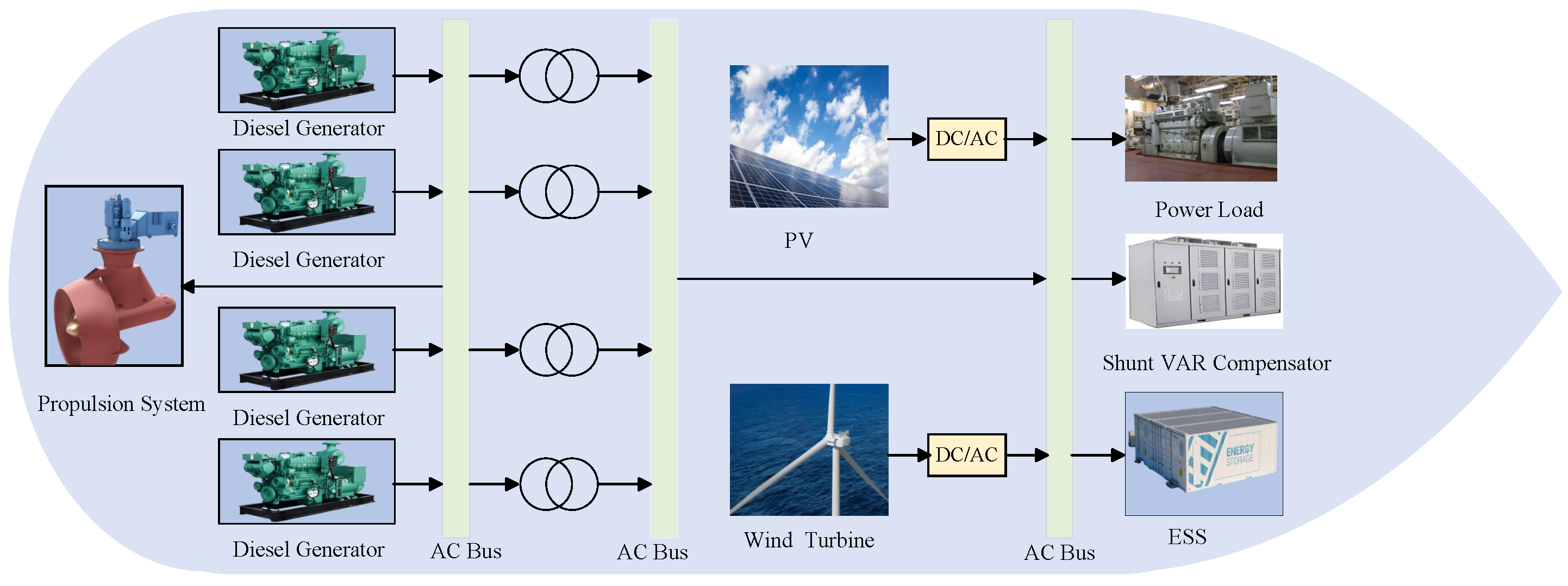
2.2. Hybrid-Energy Ship System Model

In this section, the HESPS, including diesel generator, ESS, propulsion system, PV system, and wind power system, is established. The system structure of the HESPS is shown in Figure 1. It is a medium-voltage AC power system with 18 bus nodes  [25], which includes four generators, four transformers, 17 transmission lines, a wind farm, one photovoltaic power station, six loads, and two medium-voltage main distribution boards.

2.2.1. Diesel Generator System

As the main power source for the hybrid-energy ship system, diesel generators typically supply energy when the output from PV, wind power, and ESS are insufficient to maintain the power balance. The corresponding relationship between generator cost and output power is given as follows [10]:

$$F_{gn}(t)={\alpha }_{gn}{(P_{gn}(t))}^2+{\beta }_{gn}(P_{gn}(t))+{\gamma }_{gn}$$

(4)

2.2.2. Energy Storage System

In order to improve the safety and reliability of the ship’s power system and extend the service life of the generator, an energy storage system is introduced into the ship’s power system. The introduction of a energy storage system can realize peak shaving and valley filling by adjusting the peak-to-valley characteristics of the load, thereby reducing the burden on diesel generators and improving the stability of the ship’s power system. The charging and discharging process of the energy storage system is defined as follows [15]:

$$E_e(t)=\left\{\begin{array}{cc}{E}_e(t-1)-P_e(t){\eta }_{in}\Delta t\hfill & P_e(t)\le 0\hfill \\ E_e(t-1)-{\displaystyle \frac{P_e(t)}{{\eta }_{out}}}\Delta t\hfill & P_e(t)>0\hfill \end{array}\right.$$

(5)

The operational costs of the ESS are given as follows:

$$F_e(t)={\alpha }_e{(P_e(t))}^2+{\gamma }_e\Delta t$$

(6)

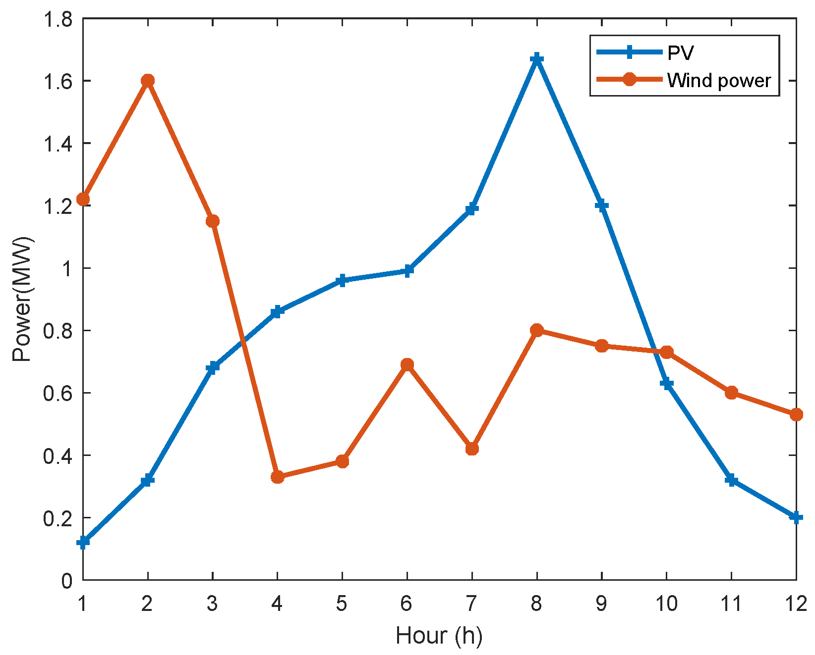
2.2.3. Wind Power System

The integration of a wind power system into the ship power system can further decrease operational costs. The output power of the wind generation system is given as follows [26]:

$$P_w(t)=\left\{\begin{array}{cc}0\hfill & 0\le v_w(t)<v_w^c\hfill \\ P_w^r(t){({\displaystyle \frac{v_w(t)}{v_w^r}})}^3\hfill & v_w^c\le v_w(t)\le v_w^r\hfill \\ P_w^r\hfill & v_w^r\le v_w(t)<v_w^o\hfill \\ 0\hfill & v_w(t)>v_w^o\hfill \end{array}\right.$$

(7)

2.2.4. Photovoltaic System

The integration of PV into the ship power system can significantly reduce operational costs. The corresponding output power is given as follows [27]:

$$P_{pv}(t)={\eta }_{pv}{A}_{pv}I(t)$$

(8)

2.2.5. Propulsion System

The power required for ship propulsion is primarily utilized to counteract resistance encountered during navigation. There exists a certain relationship between propulsion power and ship speed, which is given as follows [15]:

$$P_{pr}(t)={ϵ}_{1}V{(t)}^{{ϵ}_2}.$$

(9)

2.3. The Problem of Joint Secure Optimization of Optimal Power Flow and Voyage for HESPS

This paper aims to achieve the secure optimization of hybrid ship power systems to minimize operating costs and power losses. To solve this problem, an anomaly data detection and recovery model based on WOA-CNN-LSTM was developed to ensure the data security of optimal scheduling. Subsequently, the optimal scheduling problem of the hybrid-energy ship power system is modeled as a constrained nonlinear multi-objective optimization problem. Among them, operating costs and power losses are taken as optimization goals, and the whole system also needs to meet the constraints of carbon emissions, power, and voltage to ensure the safety, economy, and environmental protection of ship operation. Objective functions and constraints are defined below.

Objective 1: Operational costs

$$\begin{array}{cc}\hfill F_{cost}=& \sum _{t=1}^T\sum _{n=1}^{N_g}{F}_{gn}(t)+\sum _{t=1}^T{F}_e(t)\hfill \end{array}$$

(10)

Objective 2: Power loss

$$P_{loss}=\sum _{t=1}^T\sum _{k=1}^{N_a}{G}_{ij(k)}[U_i{(t)}^2+U_j{(t)}^2-2U_i(t)U_j(t)cos({\delta }_i(t)-{\delta }_j(t))]$$

(11)

Based on Equations (10) and (11), the multi-objective optimization problem can be defined as below:

$$min\left\{\begin{array}{c}{F}_1=F_{cost}\hfill \\ F_2=P_{loss}\hfill \end{array}\right.$$

(12)

2.3.1. Generator Constraints

$$P_{gn}^{min}\le P_{gn}(t)\le P_{gn}^{max}$$

(13)

$$Q_{gn}^{min}\le Q_{gn}(t)\le Q_{gn}^{max}$$

(14)

$$U_{gn}^{min}\le U_{gn}(t)\le U_{gn}^{max},i\subseteq N$$

(15)

$$-R_{gn}^{max}\le R_{gn}(t)\le R_{gn}^{max}$$

(16)

$$R_{gn}(t)=P_{gn}(t)-P_{gn}(t-1)$$

(17)

2.3.2. Energy Storage System Constraints

$$P_e^{min}\le P_e(t)\le P_e^{max}$$

(18)

$$-R_e^{max}\le R_e(t)\le R_e^{max}$$

(19)

$$E_e^{min}\le E_e(t)\le E_e^{max}$$

(20)

2.3.3. Transformer Constraint

$$K_T^{min}\le K_T(t)\le K_T^{max}$$

(21)

2.3.4. Shunt VAR Compensator Constraint

$$Q_c^{min}\le Q_c(t)\le Q_C^{max}$$

(22)

2.3.5. Ship Velocity Constraint

$$V^{min}\le V(t)\le V^{max}$$

(23)

2.3.6. Voyage Distance Constraint

$$\sum _{t\subseteq T}V(t)\Delta t=D$$

(24)

2.3.7. Power Balance Constraints

$$P_i-U_i\sum _{j=1}^N(G_{ij}cos{\delta }_{ij}+B_{ij}sin{\delta }_{ij})=0$$

(25)

$$Q_i-U_i\sum _{j=1}^N(G_{ij}sin{\delta }_{ij}-B_{ij}cos{\delta }_{ij})=0$$

(26)

2.3.8. Greenhouse Gas Emission Constrains

$${\displaystyle \frac{{\sum }_{t\in T}{F}_{C{O}_2}(t)}{{ϵ}_{3}V(t)\Delta t}}\le EEO{I}^{max},\forall n\in N,\forall t\in N.$$

(27)

$$F_{C{O}_2}(t)=a_{gn}{P}_{gn}(t)+b_{gn}{P}_{gn}(t)+c_{gn}$$

(28)

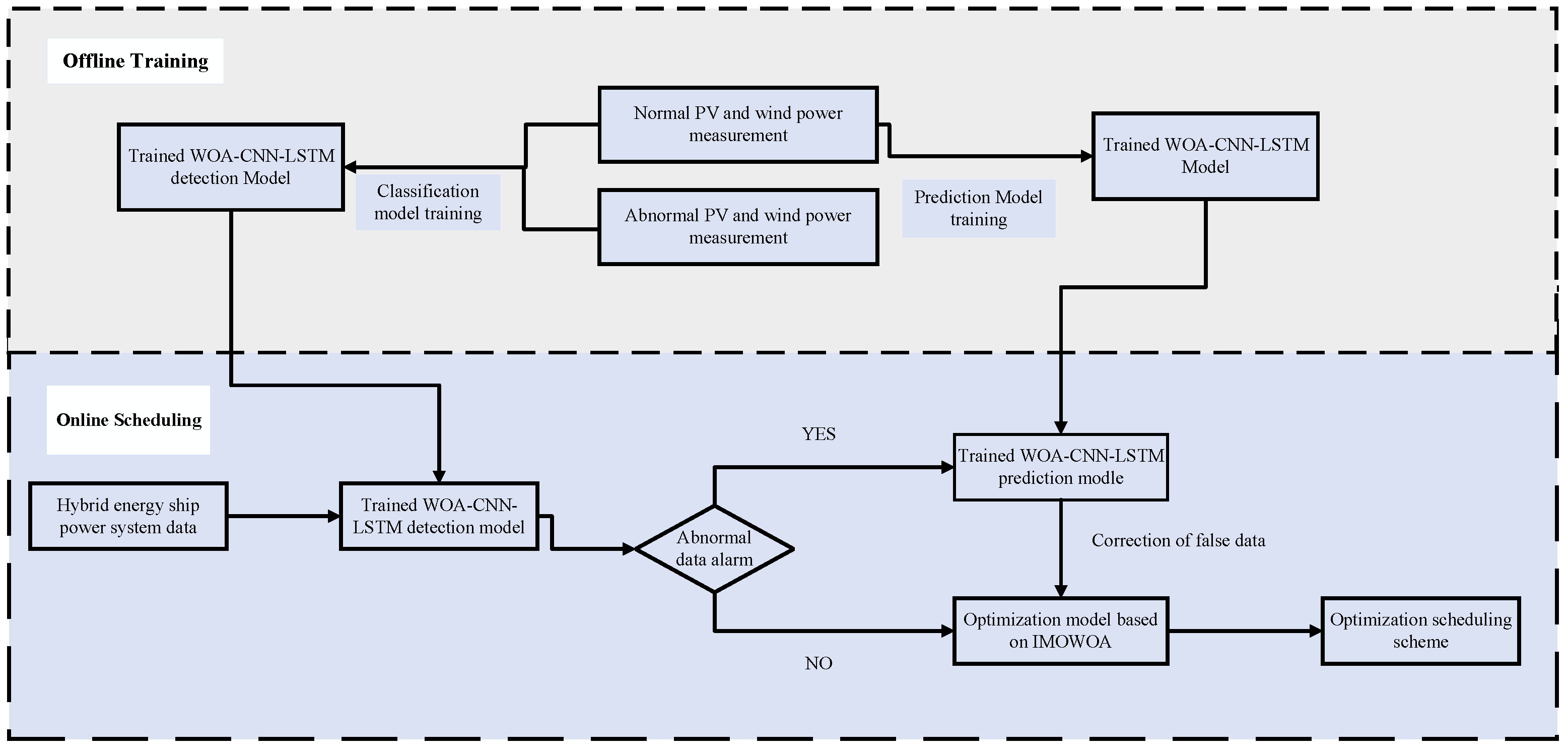
3. A Two-Stage Secure Optimization Dispatch Framework for HESPS Under FDIAs

In this section, a two-stage safety optimization model framework for the hybrid-energy ship power system is proposed, as shown in Figure 2. The framework consists of two parts: (1) an anomaly data detection and recovery model based on WOA-CNN-LSTM; (2) the optimal scheduling model based on the improved multi-objective whale algorithm. The operation process can be divided into two stages, namely the offline training stage and the online scheduling stage. In the offline training stage, the anomaly data detection model and recovery model of WOA-CNN-LSTM were trained by using the anomaly dataset and the normal dataset, respectively. In the online scheduling stage, the trained model is used to detect and recover the abnormal data generated by false data injection attacks during the operation of the ship’s power system, so as to ensure the safety and reliability of the data. Then, the corrected data is input into the scheduling model, and the improved multi-objective whale algorithm is used to realize the optimal scheduling of the the hybrid-energy ship power system. The various parts of the framework are detailed below.

3.1. WOA-CNN-LSTM Detection and Recovery Model

In order to solve the problem of abnormal data detection and recovery of the ship’s power system, this section establishes an abnormal data detection and recovery model based on WOA-CNN-LSTM. In the process of operation, the data center first uses the detection model to detect anomalies in the measured data. When the abnormal data is identified, the recovery model is randomly invoked for data correction to ensure data reliability. The construction of the WOA-CNN-LSTM model is given in detail.

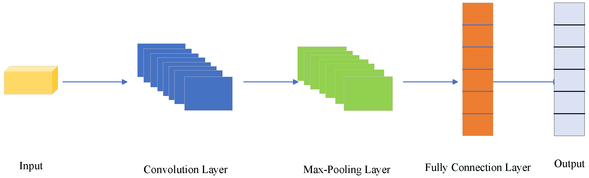
3.1.1. Convolutional Neural Network (CNN)

The CNN model consists of an input layer, convolutional layer, pooling layer, fully connected layer, and output layer [28]. The convolutional layer can utilize multiple convolutional kernels to process the input data for facilitating feature extraction. Meanwhile, the pooling layer can perform a pooling operation that reduces the dimensionality of the data and enhances the further feature extraction. The structure of the CNN is illustrated in Figure 3. By constructing the CNN model, the spatial features of PV and wind energy data can be extracted. The corresponding description of the CNN model is given as follows:

$$Y=f(x\ast W+b)$$

(29)

where Y denotes the output of the convolution operation, f denotes the activation function, x denotes the input data of input layer, W denotes the weight matrix, and b denotes the bias vector.

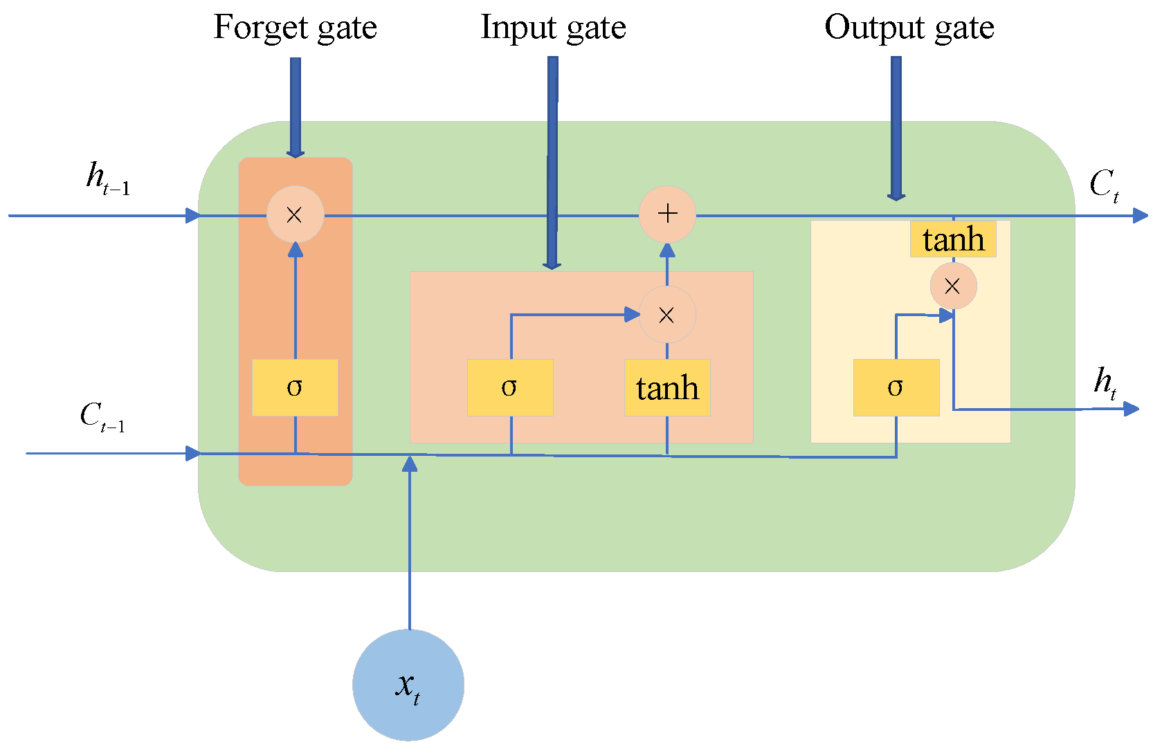
3.1.2. Long Short-Term Memory Neural Network Model

The LSTM [29] model consists of a forget gate, input gate, and output gate, by which temporal features of PV and wind energy data can be extracted. The structure of the LSTM is shown in Figure 4. The mathematical description for the LSTM can be defined as follows:

Forget gate: The forget gate is responsible for discarding the unimportant information from the preceding cell unit, which can be defined as follows:

$$f_t=f(W_{fh}{h}_{t-1}+W_{fx}{x}_t+b_f)$$

(30)

where $f_t$ denotes the output; f is the activation function; $W_{fh}$, $W_{fx}$ denote the weight matrix of the forget gate; $h_{t-1}$ denotes the hiden state of time $t-1$; $x_t$ denotes the input; and $b_f$ denotes the bias vector.

Input gate: The input gate determines how much new information can be added into the cell state, which can be described as follows:

$$i_t=f(W_t·[h_t,x_t]+b_t)$$

(31)

$${\tilde{C}}_t=tanh(W_c·[h_{t-1},x_t]+b_c)$$

(32)

where $i_t$ denotes the output of the input gate; $W_t$, $W_c$ denote the weight matrix; $b_t$, $b_c$ denote the bias vector; and ${\tilde{C}}_t$ denotes the temporary cell state.

The old cell state $C_t$ is multiplied with $f_t$ to discard the unwanted information. Then, the temporary cell state $\widetilde{C_t}$ will be added to generate the new cell state $C_t$. It can be defined as follows:

$$C_t=f_t{C}_{t-1}+i_t\widetilde{C_t}$$

(33)

Output gate: The output gate determines the output based on the updated cell state. The update equation is defined as follows:

$$o_t=f(W_o·[h_{t-1},x_t]+b_o)$$

(34)

where $o_t$ denotes the output of the output gate; $W_o$ denotes the weight of the matrix; and $b_o$ denotes the bias vector. After the cell state $C_t$ of the current time step is processed, a value between −1 and 1 will be generated. This value combined with the output gate output will generate a hidden state $h_t$ for the current time step, which is defined as follows:

$$h_t=o_{t}tanh(C_t)$$

(35)

Remark 1. 

The CNN model can effectively extract useful features in ship PV or wind power, and improve the computational efficiency, while the LSTM can effectively deal with long time series data, avoid the problem of gradient explosion, and effectively learn the relationship between time series data.

3.1.3. Whale Optimization Algorithm

The WOA can improve the prediction accuracy and increases the robustness of the CNN-LSTM model by automatically searching for the optimal combination of hyperparameters. The WOA is a bio-inspired meta-heuristic algorithm, which simulates the hunting strategy of humpback whales [30]. The whole process of the algorithm includes three behavioral strategies: the searching mechanism, encircling mechanism, and bubble net attacking.

Searching prey: At this stage, a random individual from the population is selected as the search agent. It can guide the other whale individuals to ensure comprehensive exploration of the target space. The updated formula is defined as follows:

$$X_i(t+1)=X_{rand}(t)-A\ast D$$

(36)

$$D=|C\ast X_{rand}(t)-X_i(t)|$$

(37)

where t is the number of the iteration, $X_{rand}$ is the position vector of the randomly selected whale individual, $X_i(t)$ is position vector of the ith whale individual, and A and C are the coefficients, which are given as follows:

$$A=2\ast a\ast r-a$$

(38)

$$a=2-2\ast t/t_{max}$$

(39)

$$C=2\ast r$$

(40)

where r is a random value in [0, 1], a is a coefficient that decreases linearly from 2 to 0, and $t_{max}$ is the maximum number of iterations.

Encircling prey: At this stage, the individual in the optimal position relative to the optimal solution is defined as the optimal search agent. Then, the optimal search is used to guide the other whale individuals. The updated formula is defined as follows:

$$D=|C\ast X_{best}(t)-X_i(t)|$$

(41)

$$X_i(t+1)=X_{best}(t)-A\ast X_i(t)$$

(42)

where $X_{best}(t)$ is the position vector of the optimal search agent at present.

Bubble net attacking: At this stage, the spiral and shrinking mechanism are adopted to update the position of the individual. The updated formula is defined as follows:

$$D^{\prime }=|X_{best}-X_i(t)|$$

(43)

$$X_i(t+1)=D^{\prime }\ast e^{b\ast l}\ast cos(2\pi l)+X_i(t)$$

(44)

where b denotes a constant that denotes the shape of the log helix, and l denotes a random value between −1 and 1.

Remark 2. 

Considering that the difficulty in choosing the hyperparameters of the current model limits the performance of the model, this paper adopts WOA to optimize the hyperparameters of the model, which has the advantages of simple parameters and fast computing speed, and when used to optimize the hyperparameters of the model, it is able to find better hyperparameters faster, which can further improve the generalization ability of the CNN-LSTM detection and prediction model.

3.2. False Data Identification Based on WOA-CNN-LSTM Detection Model

As shown in Figure 2, the SCADA will collect data (PV, wind and generator, etc.) from the ship’s power grid for safety testing. The false data identification process can be framed as a multi-label classification problem. In this context, $M_{input}^t=(M_{input}^t(1),M_{input}^t(2),\dots ,M_{input}^t(n))$ represent the input measurement vector; $L_{input}^t=(L_{input}^t(1),L_{input}^t(2),\dots ,L_{input}^t(n))$ denote the label of the measurement vector; and $M_{output}^t=(M_{output}^t(1),M_{output}^t(2),\dots ,M_{output}^t(n))$ indicate the data classification results following detection and identification. When the measurement vector at time (t) is identified as containing abnormal data, the classification label is assigned a value of 1; otherwise, it is assigned a value of 0, which is specified as follows:

$$M_{input}^t=\left\{\begin{array}{c}1,abnormaldata\hfill \\ 0,otherwise\hfill \end{array}\right.$$

(45)

Typically, as discussed in Section 2.1 regarding the detection threshold $\tau$, if the threshold $\tau$ is set too high or too low, it may result in an increased rate of misdetection and omission rate. Consequently, the detection threshold is conventionally set at 0.5 [8]. In the context of multi-label classification problems, the cross-entropy loss function is introduced to obtain optimal model learning parameters. It is defined as follows:

$$L(\theta )={\displaystyle \frac{1}{num}}\sum _{n=1}^N=-[M_{output}^t(n)log(M_{input}^t(n))+(1-M_{output}^t(n))log(1-M_{input}^t(n))]$$

(46)

3.3. False Data Recovery Based on WOA-CNN-LSTM Prediction Model

If the SCADA detects the injected false measurement data $A_m=[A_m(1),A_m(2),\dots ,$$A_m(n)]$, the day-ahead prediction model using WOA-CNN-LSTM is triggered. Based on the historical measurement vector $H_m=[H_m(1),H_m(2),\dots ,H_m(n)]$, the WOA-CNN-LSTM prediction model will generate the measurement data y to replace the false data. In the context of prediction problems, the RMSE loss function is introduced to obtain optimal model learning parameters. It is defined as follows:

$$RMSE=\sqrt{{\displaystyle \frac{1}{n}}\sum _i^n(\widehat{y_i}-y_i)}$$

(47)

Remark 3. 

Since ship photovoltaic or wind power data are generally long time series data, and at the same time, the data may contain multiple features, the traditional single model may have an insufficient ability to extract the features, or there may be a problem of gradient explosion when dealing with long time series data. In this paper, an WOA-CNN-LSTM spatio-temporal model is developed, which can effectively identify abnormal data and achieve data recovery through prediction under FDIAs, thus ensuring the safe and optimal scheduling of the HESPS.

3.4. Optimization Scheduling Model Based on Improved Multi-Objective Whale Optimization Algorithm

In order to improve the economic and environmental sustainability of the HESPS, an IMOWOA-based optimization model is developed as follows.

Improved Multi-Objective Whale Optimization Algorithm

The IMOWOA is developed by hybridizing MOWOA with crisscross optimization (CSO) [31], which consists of the whale operator, horizontal crossover operator, vertical crossover operator, and opposition-based learning strategy. The offspring population generated by these operators are called the moderation solution set, which are expressed as $M_{woa}$, $M_{hc}$, $M_{vc}$, respectively. The moderation solution set will compete with its parent population to form a new population. Then, the archive method in reference [32] is used to preserve the solution set. The specific improvement process is as follows.

Whale operator: The whale operator introduces a differential variation strategy into the whale algorithm. The search capabilities of the differential algorithm enhance the global search efficiency of the whale algorithm and improve population diversity [33]. The whale algorithm is executed according to Equations (36)–(42). Subsequently, the differential variation strategy is applied with a specified probability across all dimensions of the individual, which can be defined as follows:

$$M_{woa,i}(t+1)=X_i(t)+F\ast (X_{r1}+X_{r2})$$

(48)

$$F=F_{min}-(F_{max}-F_{min})\ast (t/t_{max})$$

(49)

where the $M_{woa,i}(t+1)$ denotes the moderation solution, $X_{r1}$ and $X_{r2}$ are two random individuals in the paternal population, F is a scaling factor whose value is between 0 and 1.5 in this paper, $F_{min}$ and $F_{max}$ are the minimum and maximum values of F.

Horizontal crossover operator: Horizontal crossing is an operation performed on all the dimensions of two different individuals [31]. Horizontal crossing can search for new solutions in a hypercube formed by two parent individuals. In addition, the periphery of the hypercube can be searched with a certain probability, thus reducing the search blind spots. The horizontal crossover is defined as follows:

$$\begin{array}{cc}\hfill M_{hc}(n_1,j)=& r_1·X(n_1,j)+(1-r_1)·X(n_2,j)+c_1\ast (X(n_1,j)-X(n_2,j))\hfill \end{array}$$

(50)

$$\begin{array}{c}\hfill M_{hc}(n_2,j)=r_2·X(n_2,j)+(1-r_2)·X(n_1,j)+c_2\ast (X(n_2,j)-X(n_1,j))\end{array}$$

(51)

where $M_{hc}(n_1,j)$ and $M_{hc}(n_2,j)$ are the offspring of $X(n_1,j)$ and $X(n_2,j)$, respectively; $r_1$ and $r_2$ are uniformly distributed value between 0 and 1; and $c_1$ and $c_2$ are uniformly distributed values between −1 and 1.

Vertical crossover operator: Vertical crossover can effectively ensure population diversity and avoid the populations falling into local optima [31]. The vertical crossover operator operates on two different dimensions inside an individual, which can be defined as follows:

$$M_{vc}(n,j)=r·X(n,j_1)-(1-r)·X(n,j_2)$$

(52)

where $M_{vc}(n,j)$ denotes the moderation solution generated by the $X(n,j_1)$ and $X(n,j_2)$, and r denotes the uniformly distributed value between 0 and 1.

Opposition-based learning strategy: The opposition-based learning strategy was proposed by Li M. [34], and its adoption can facilitate the generation of a good initial population. The opposition-based learning strategy is defined as follows:

$$X(i,j)=U_b(j)+(U_b(j)-L_b(j))\ast rand$$

(53)

$$OX(i,j)=U_b(j)+L_b(j)-X(i,j)$$

(54)

where $OX$ denotes the position vector of the new individual generated by the opposition-based learning strategy, $U_b$ and $L_b$ denote the upper bound and lower bound, and $rand$ denotes the uniformly distributed value between 0 and 1.

In conclusion, by hybridizing the WOA with the CSO and adopting the opposition-based learning strategy and differential variant strategies, an improved multi-objective whale optimization algorithm is proposed in this section. In comparison to the traditional multi-objective whale optimization algorithm, the IMOWOA can more comprehensively explore the entire target space during the iterative process. Simultaneously, it maintains a high level of population diversity, which helps prevent the population from converging to local optima, thereby enhancing its effectiveness in solving the joint optimization of the hybrid-energy ship’s voyage and optimal power flow.

3.5. The Proposed Secure Two-Stage Optimization Dispatch Algorithm for HESPS

Due to the increasing consumption of fossil fuels in the shipping industry and the increasingly stringent emission regulations, hybrid-energy ships are gaining traction. Compared with traditional diesel ships, hybrid-energy ships can make full use of photovoltaic and wind energy, thereby reducing the fuel consumption and carbon emissions of ships. However, new energy also increases the complexity and operational vulnerability of hybrid-energy ships, which makes the optimal scheduling of hybrid-energy ships face severe challenges. Therefore, this chapter develops a two-stage safe optimal scheduling framework for hybrid-energy ships, based on the method described above. Its operation steps and pseudocode are given below, and the pseudocode is shown in Algorithm 1.

Algorithm 1 The secure two-stage optimization scheduling algorithm for HESPS

1: // Stage 1: Offline training stage   2: Input the offline ship power system dataset: PV, wind power, etc.   3: Dataset process.   4: for t to $maxepoch$ do   5:    Update the hyper-parameter using the WOA.   6:    Input the updated hyper-parameter and dataset.   7:    Train the prediction model based on CNN-LSTM.   8: end for   9: Output the trained WOA-CNN-LSTM detection and recovery model. 10: // Stage 2: Online scheduling stage. 11: Input the trained WOA-CNN-LSTM detection and recovery model. 12: Input the real-time ship power system data. 13: if $M_{input}^t==1$ then 14:    Abnormal data recovery. 15:    Output the repaired data. 16: else if $M_{input}^t==0$ then 17:    Output the real-time data. 18: end if 19: // Algorithm initialization. 20: Input the PV, wind power, system parameter, etc. 21: Set algorithm parameter. 22: Initialize population X according to Equations (53) and (54) and initialize a, A, C, F, p. 23: Calculate the fitness value and obtain the initial Pareto frontier. 24: // Main loop 25: for t to $t_{max}$ do 26:    Perform the whale operator to update the $M_{woa}$ according to Equations (36)–(44), (48) and (49). 27:    Update the population X. 28:     Run horizontal crossover operator and update $M_{hc}$ according to Equations (50) and (51). 29:    Update the population X. 30:    Run vertical crossover operator and update $M_{vc}$ according to Equation (52). 31:    Update the population X 32:    Update the Pareto frontier and archive. 33: end for 34: return Output solution and Pareto frontier.

• Step 1: Train the offline WOA-CNN-LSTM detection and recovery model;
• Step 2: WOA-CNN-LSTM-based data detection and recovery;
• Step 3: Establish the system model of HESPS according to Equations (4)–(9);
• Step 4: Initialize the related parameters, such as ESS, PV, etc.;
• Step 5: Calculate the operational cost, power loss, and EEOI according the Equation (10), Equation (11), and Equation (27), respectively;
• Step 6: Search for the Pareto front by using the IMOWOA;
• Step 7: Output the optimal optimization solution for cost, power loss, etc.

3.6. Discussion of the Application of the Proposed Method to a Real System

The challenges faced in implementing the detection system primarily include computational latency and data quality dependence. Deep learning models like WOA-CNN-LSTM and multi-objective optimization techniques such as IMOWOA may introduce significant delays, which can be mitigated by deploying lightweight models, such as quantized CNN-LSTM, on edge devices and utilizing federated learning to distribute computational loads across nodes; additionally, the accuracy of detection relies heavily on the representativeness of historical data, a challenge that can be addressed by augmenting the training dataset with adversarial samples generated using generative adversarial networks (GANs) to simulate false data injection attacks (FDIAs) and implementing online learning mechanisms to enable the model to dynamically adapt to emerging attack patterns.

4. Case Analysis

In this section, the performance of the proposed two-stage optimal scheduling model for hybrid-energy ship power systems will be tested to verify the effectiveness of the proposed method.

Table 1. Hybrid-energy ship parameter setting.

	${\mathit{G}}_1$	${\mathit{G}}_2$	${\mathit{G}}_3$	${\mathit{G}}_4$	ESS	PV	Wind Power
Minimum power (MW)	2	2	3	3	−3	0	0
Minimum power (MW)	10	10	20	20	3	3	3
Maximum ramp rate	5	5	5	5	1	-	-
Cost function parameter	${\alpha }_{g1}$ = 13	${\alpha }_{g2}$ = 13	${\alpha }_{g3}$ = 5.2	${\alpha }_{g4}$ = 5.2	${\alpha }_e$ = 4.3	-	-
	${\gamma }_{g1}$ = 12	${\gamma }_{g2}$ = 12	${\gamma }_{g3}$ = 52	${\gamma }_{g4}$ = 5.2	${\gamma }_e$ = 1	-	-
	${\beta }_{g1}$ = 430	${\beta }_{g2}$ = 430	${\beta }_{g3}$ = 340	${\beta }_{g4}$ = 340	-	-	-
CO2 function parameter	$a_{g1}$ = 13.5	$a_{g12}$ = 13.5	$a_{g3}$ = 5.2	$a_{g4}$ = 5.2	-	-	-
	$b_{g1}$ = 10	$b_{g2}$ = 10	$b_{g3}$ = 58	$b_{g4}$ = 58	-	-	-
	$c_{g1}$ = 450	$c_{g2}$ = 450	$c_{g3}$ = 390	$c_{g4}$ = 390	-	-	-

shows the specific parameters of the power system model of hybrid-energy ships. The datasets for PV and wind power were sourced from a PV plant and an offshore wind farm in Europe. The fault data used in this paper are simulated data, which are generated in a MATLAB2024A environment on the basis of normal data. The anomaly dataset used for detection in this paper includes a total of 8737 pieces of data, of which the ratio of normal data to abnormal data is 3:1. The anomalous dataset will be used to train the WOA-CNN-LSTM classifier model, while the normal dataset will be used to train the WOA-CNN-LSTM prediction model. All models are optimized by the whale algorithm to enhance the generalization ability and stability of the model.

The simulation was performed on a laptop equipped with an i5-1035G1 CPU model and a NVIDIA GeForce MX 230 GPU model. MATLAB-R2022b and Python 3.9 were used to implement FDIA detection, data recovery, and optimal scheduling based on IMOWOA.

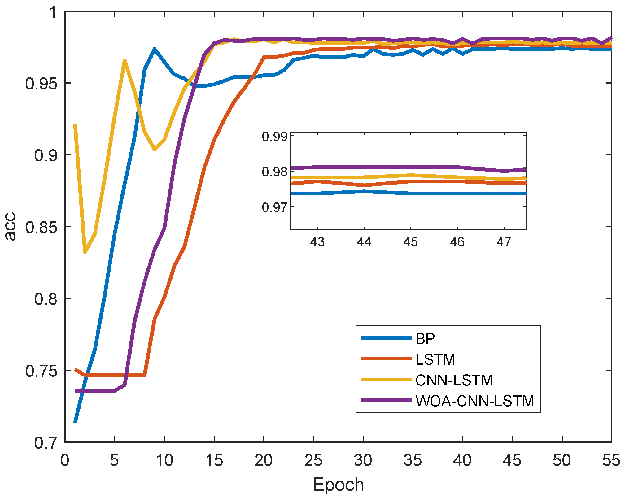
4.1. Performance Test for Identification of False Data Under FDIAs

This paper compares four detection models: BP neural network, LSTM, CNN-LSTM, and the WOA-CNN-LSTM hybrid model. The detailed parameter configurations for each model are provided in

Table 2. The parameters of the abnomal data detection model.

Model	Number of Hidden Layers	Number of Hidden Layer Neurons	Learning Rate	Epoch
BP	2	layer 1 = 10; layer 2 = 10	0.001	55
LSTM	2	layer 1 = 10; layer 2 = 10	0.001	55
CNN-LSTM	2	CNN: layer 1 = 10; layer 2 = 10 LSTM: layer 1 = 10; layer 2 = 10	0.001	55
WOA-CNN-LSTM	2	CNN: layer 1 = 7; layer 2 = 14 LSTM: layer 1 = 16; layer 2 = 13	0.001	55

. To evaluate the performance of the proposed WOA-CNN-LSTM detection model, the following evaluation indicators, including accuracy (acc), precision (pre), recall (rec), and $f_{1}score$ ($f_1$), are defined as follows:

$$acc={\displaystyle \frac{tpr+tnr}{tpr+tnr+fpr+fnr}}$$

(55)

$$pre={\displaystyle \frac{tpr}{tpr+fpr}}$$

(56)

$$rec={\displaystyle \frac{tpr}{tpr+fnr}}$$

(57)

$$f_1={\displaystyle \frac{2\ast pre\ast rec}{pre+rec}}$$

(58)

where tpr denotes the true positive rate; tnr denotes the true negative rate; fpr denotes the false positive rate; and fnr denotes the false negative rate.

After evaluating each model, the comparative results are summarized in the following tables:

Table 3. Comparative results of false data detection under different detection models.

Method	pre	rec	${\mathit{f}}_1$
BP	0.9788	0.9181	0.9475
LSTM	0.9718	0.9323	0.9516
CNN-LSTM	0.9624	0.9464	0.9546
Method in [35]	0.9812	0.9462	0.9712
Method in [36]	0.9723	0.9428	0.9613
WOA-CNN-LSTM	0.9864	0.9437	0.9646

presents the detection performance of the four models on anomalous data;

Table 4. Comparison of model running stability analysis.

Method	min	max	Average	std
BP	0.9691	0.9737	0.9720	0.0016
LSTM	0.9703	0.9760	0.9733	0.0018
CNN-LSTM	0.9708	0.9777	0.9737	0.0022
WOA-CNN-LSTM	0.9777	0.9817	0.9800	0.0014

compares the operational stability across the four models; and Figure 5 illustrates the accuracy (acc) iteration curves for each model.

The proposed detection model demonstrates superior performance over baseline methods (BP, LSTM, and CNN-LSTM), achieving a precision (Pre) of 0.9864, recall (Rec) of 0.9437, and F1-score (F1) of 0.9646. However, while our model exhibits higher accuracy than those in [35,36], its F1-score remains marginally lower. To overcome this limitation, future improvements should not only incorporate the model features from [35,36] but also explore integrating a foundational tabular model with semantic object-aware representations [37] and a Dempster–Shafer-based multi-echo state network [38].

As evidenced by Table 4, the proposed detection model demonstrates significantly higher stability in identifying anomalous data compared to existing models. Specifically, the WOA-CNN-LSTM hybrid model developed in this study enables rapid and efficient detection of FDIAs. Furthermore, Figure 5 clearly shows that the accuracy curve of the proposed model consistently surpasses those of benchmark models, with quantitatively superior accuracy values across all test scenarios.

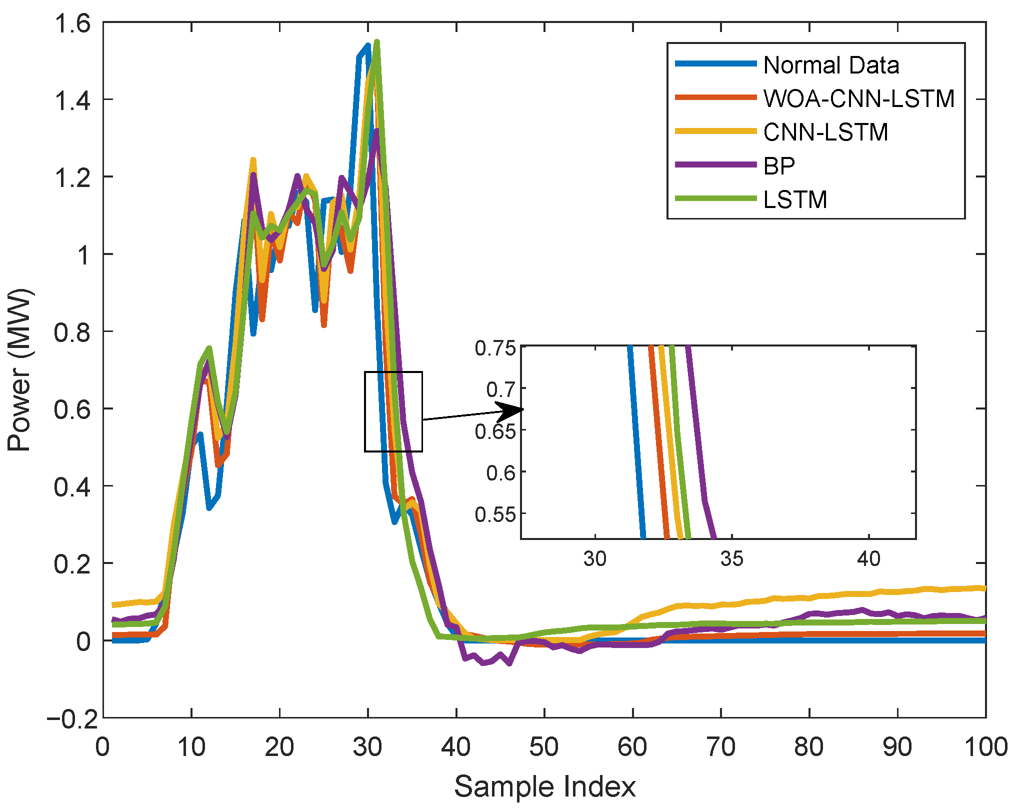
4.2. Performance Test for Data Recovery Based on WOA-CNN-LSTM Prediction Model

In this section, the performance of the proposed WOA-CNN-LSTM prediction model for anomaly data recovery is tested. To verify the effectiveness of this method, the WOA-CNN-LSTM model is compared with BP, LSTM, and CNN-LSTM, with specific parameters of each model shown in

Table 5. The parameters of the abnomal data recovery model.

Model	Number of Hidden Layers	Number of Hidden Layer Neurons	Learning Rate	Epoch
BP	2	layer 1 = 10; layer 2 = 10	0.01	30
LSTM	2	layer 1 = 10; layer 2 = 10	0.01	30
CNN-LSTM	2	CNN: layer 1 = 10; layer 2 = 10 LSTM: layer 1 = 10; layer 2 = 10	0.01	30
WOA-CNN-LSTM	2	CNN: layer 1 = 63; layer 2 = 25 LSTM: layer 1 = 29; layer 2 = 31	0.0105	30

. In addition to the evaluation indexes described in Section 4.2, R-squared ($R^2$), mean squared error (MSE), and mean absolute error (MAE) are also introduced as evaluation indicators. The specific mathematical formulas are shown in Equations (59)–(61). Of note, higher values of $R^2$ and lower values of $MSE$, $RMSE$, and $MAE$ indicate better prediction results.

$$R^2=1-{\displaystyle \frac{{\sum }_i^n{(\widehat{y_i}-y_i)}^2}{{\sum }_i^n{(\overline{y}-y_i)}^2}}$$

(59)

$$MSE={\displaystyle \frac{1}{n}}\sum _i^n(\widehat{y_i}-y_i)$$

(60)

$$MAE={\displaystyle \frac{1}{n}}\sum _i^n|\widehat{y_i}-y_i|$$

(61)

Having tested each model, the following tables show comparisons of the running results of each model:

Table 6. Comparison results of data recovery under different day-ahead prediction models.

Error Evaluation Index	${\mathit{R}}^2$	RMSE	MSE	MAE
LSTM	0.9504	0.1173	0.01376	0.04983
BP	0.9379	0.1313	0.01724	0.08152
CNN-LSTM	0.9579	0.1081	0.01168	0.06864
WOA-CNN-LSTM	0.9692	0.09249	0.008553	0.04338

shows the detection performance of the above four models on abnormal data, while

Table 7. Comparison of models running stability analysis.

Method	min	max	Average	std
BP	0.8972	0.9379	0.9295	0.0123
LSTM	0.9282	0.9504	0.9398	0.0072
CNN-LSTM	0.9531	0.9579	0.9552	0.0017
WOA-CNN-LSTM	0.9676	0.9692	0.9684	0.0004

shows a comparison of the operational stability of the above four models. Figure 6 shows the comparison of the data recovery effects of each model.

As shown in Figure 6, the prediction results of the WOA-CNN-LSTM model proposed in this paper have the best fit with the actual data, and its performance is significantly better than that of the comparison model. In addition, from the quantitative analysis in Table 6, the proposed method obtained the optimal values in the evaluation indexes: the value of $R^2$ is higher than the comparison, which was 0.969; and the values of RMSE, MSE, and MAE were lower than those of the comparison model, which were 0.092, 0.0086, and 0.043, respectively. Furthermore, it can be seen from Table 7 that the stability of the recovery model proposed in this paper for the recovery ability of abnormal data is also better than that of other models. The above results show that the model has excellent prediction accuracy and can effectively correct the abnormal data caused by FDIA.

4.3. Performance Analysis of IMOWOA-Based Optimization Model

In this section, three cases are designed to verify the performance of the optimal scheduling model based on IMOWOA. Case 1 focuses on verifying the ability of IMOWOA to handle multi-objective optimization. Case 2 focuses on verifying the application effect of the model in the optimization problem of hybrid-energy ships under a fixed voyage. Case 3 aims to verify the performance of the model in solving the joint optimization problem of optimal power flow and voyage for hybrid-energy ships.

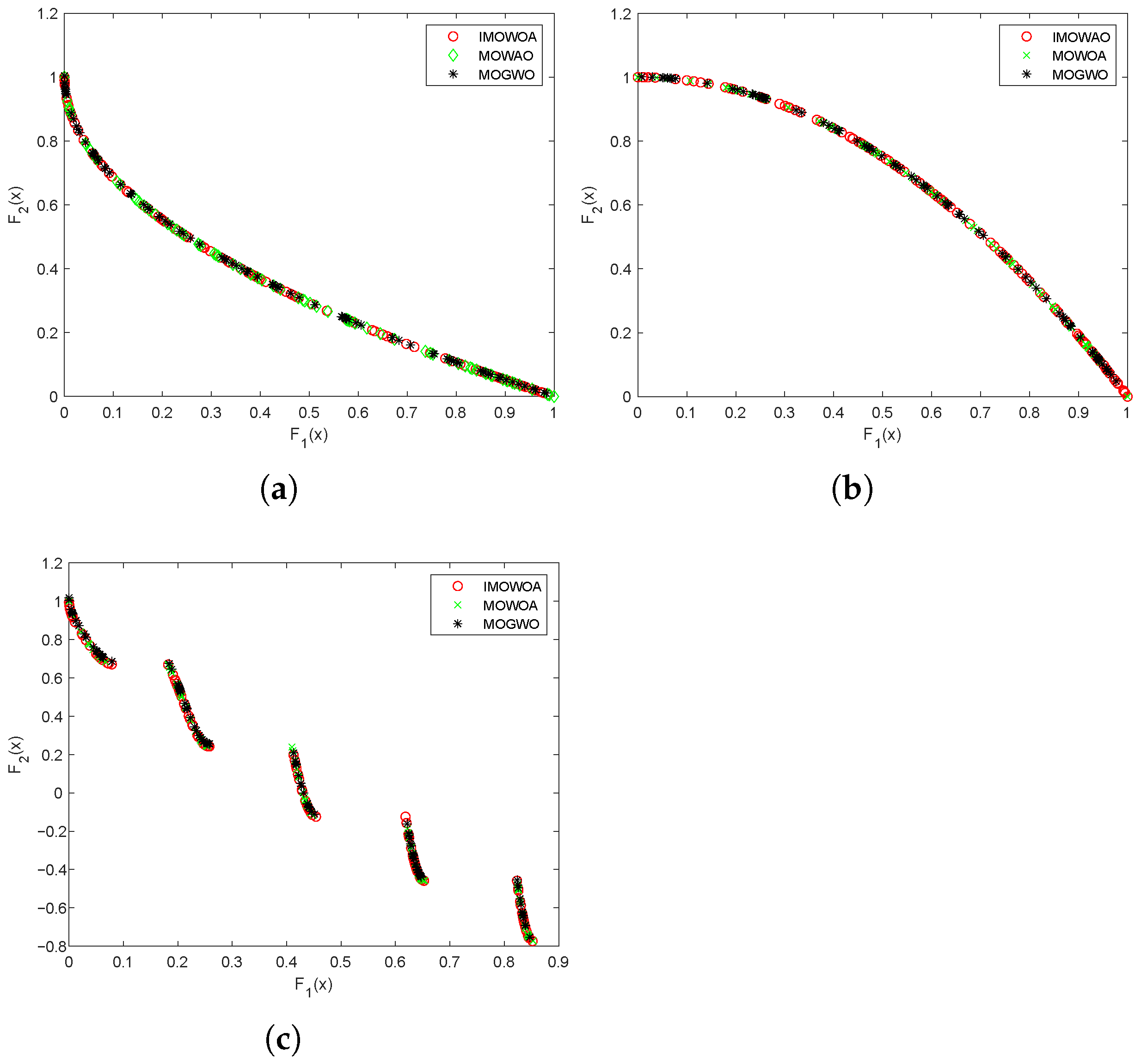
4.3.1. Performance Test of the IMOWOA

In this section, the corresponding test functions are given below:

$$ZDT1=\left\{\begin{array}{cc}min{f}_1(x)=x_1\hfill & \\ min{f}_2(x)=g(1-\sqrt{{\displaystyle \frac{f_1}{g(x)}}})\hfill & \\ g(x)=1+{\displaystyle \frac{9}{n-1}}{\sum }_{i=2}^n{x}_i\hfill & \end{array}\right.$$

(62)

$$s.t.n=30,0\le x_i\le 1,i=1,2\dots ,n$$

$$ZDT2=\left\{\begin{array}{cc}min{f}_1(x)=x_1\hfill & \\ min{f}_2(x)=g(1-({\displaystyle \frac{f_1}{g(x)}}{)}^2)\hfill & \\ g(x)=1+{\displaystyle \frac{9}{n-1}}{\sum }_{i=2}^n{x}_i\hfill & \end{array}\right.$$

(63)

$$s.t.n=30,0\le x_i\le 1,i=1,2\dots ,n$$

$$ZDT3=\left\{\begin{array}{cc}min{f}_1(x)=x_1\hfill & \\ min{f}_2(x)=g(1-\sqrt{{\displaystyle \frac{f_1}{g(x)}}}-{\displaystyle \frac{f1}{g(x)}}sin(10\pi f_1))\hfill & \\ g(x)=1+{\displaystyle \frac{9}{n-1}}{\sum }_{i=2}^n{x}_i\hfill & \end{array}\right.$$

(64)

$$s.t.n=30,0\le x_i\le 1,i=1,2\dots ,n$$

In order to evaluate the performance of IMOWOA, the multi-objective gray wolf optimization algorithm (MOGWO) [39], the multi-objective whale optimization algorithm (MOWOA) [40], and IMOWOA are compared and analyzed in this section. The parameters of each algorithm are shown in

Table 8. The parameters of the algorithms.

MOGWO	$t_{max}=200$	$popsize=100$
MOWOA	$t_{max}=200$	$popsize=100$	p = 0.5
IMOWOA	$t_{max}=200$	$popsize=100$	p = 0.5	$p_{vc}=0.7$	$F_{min}=0$	$F_{max}=1.5$

below. Hypervolume (HV), inverted generation distance (IGD), and spacing (SP) are selected as the evaluation indicators, and the specific definitions of each index are as follows.

HV measures the space dominated by the individuals; a higher HV value indicates that the solution set obtained is closer to the true Pareto frontier. Then, the HV is defined as follows:

$$HV=volume(\bigcup _{i=1}^{\left|S\right|}{v}_i)$$

(65)

where $v_i$ denotes a super volume formed by the non-dominated solution i and the reference point, and S denotes the non-dominated solution set.

The IGD represents the average distance from each solution to the nearest solution on the true Pareto frontier. A lower IGD value indicates that the obtained solution set is closer to the true Pareto front. The IGD is defined as follows:

$$IGD(P,P^{\ast })={\displaystyle \frac{{\sum }_{x\in P^{\ast }}mi{n}_{y\in P}dis(x,y)}{|P^{\ast }|}}$$

(66)

where $dis(x,y)$ denotes the euclidean distance between point x and point y.

The SP is an indicator, which can assess the distribution and depict the uniformity of the non-dominated solutions. A smaller SP value indicates a more uniform distribution of the non-dominant solution set. The SP is defined as follows:

$$SP=\sqrt{{\displaystyle \frac{1}{N-1}}\sum _{i=1}^N{(\overline{d}-d_i)}^2}$$

(67)

where $\overline{d}$ denotes the average value of all $d_i$.

Based on the above evaluation indicators, the multi-objective gray wolf optimization algorithm (MOGWO) [39], the multi-objective whale optimization algorithm (MOWOA) [40], and IMOWOA are compared and analyzed in this section. The comparison results are shown in

Table 9. The test result of ZDT1, ZDT2, and ZDT3.

Test Function	Hypervolume
	MOWOA	MOGWO	IMOWOA	Improvement
ZDT1	0.715116	0.713204	0.717313	0.306%
ZDT2	0.439386	0.434151	0.442793	0.800%
ZDT3	0.597037	0.596749	0.599100	0.344%
Test Function	IGD
	MOWOA	MOGWO	IMOWOA	Improvement
ZDT1	0.008446	0.008644	0.006017	28.759%
ZDT2	0.009478	0.009527	0.005843	38.352%
ZDT3	0.009977	0.010187	0.006706	32.846%
Test Function	SP
	MOWOA	MOGWO	IMOWOA	Improvement
ZDT1	0.011305	0.010825	0.009603	15.055%
ZDT2	0.012565	0.012972	0.008928	28.945%
ZDT3	0.016242	0.013652	0.010462	35.587%

and Figure 7.

As indicated in Table 9, HV under IMOWOA is higher compared to the other algorithms. Additionally, IGD and SP values under IMOWOA are lower than those under the other algorithms. Compared with MOWOA and MOGWO, the improvements in HV, IGD, and SP under IMOWOA were at least 0.306%, 28.759%, and 15.055%. These results indicate that the solution set obtained by IMOWOA is closer to the true Pareto frontier than those under other algorithms.

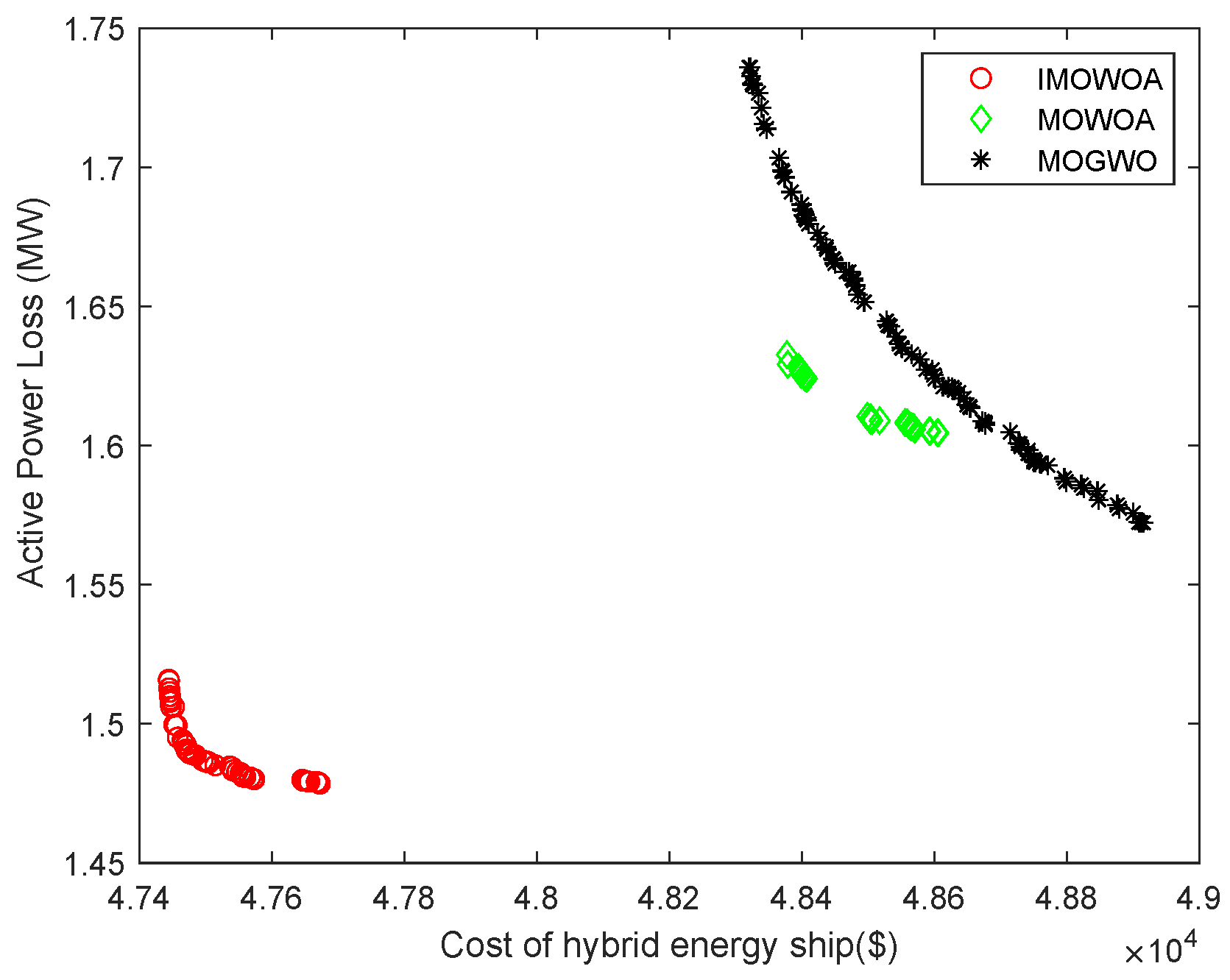
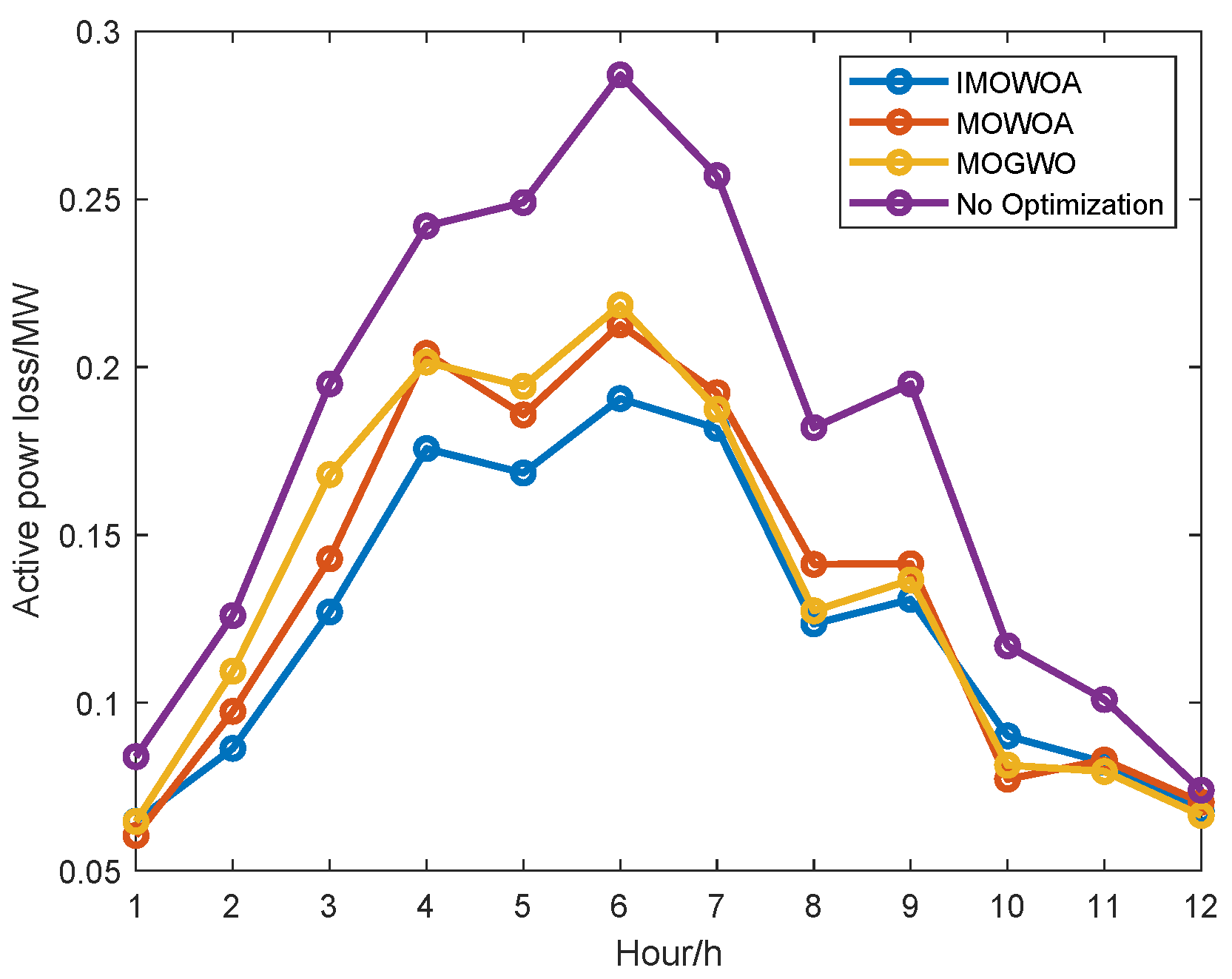
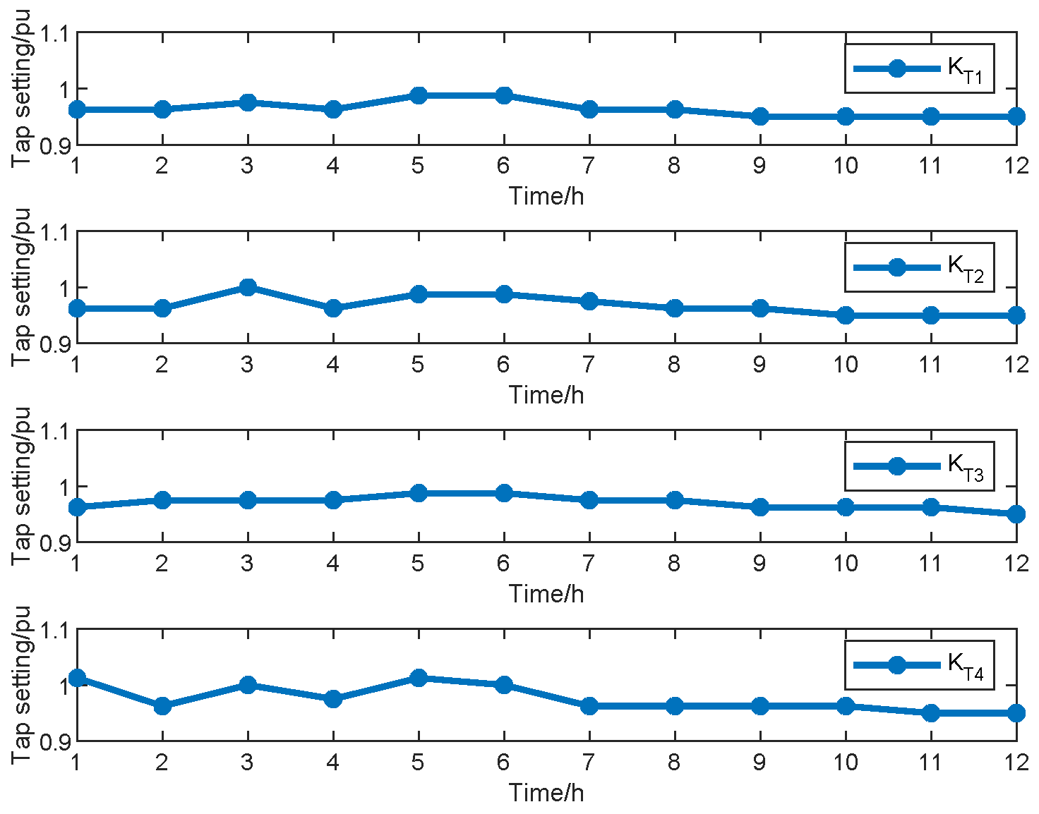
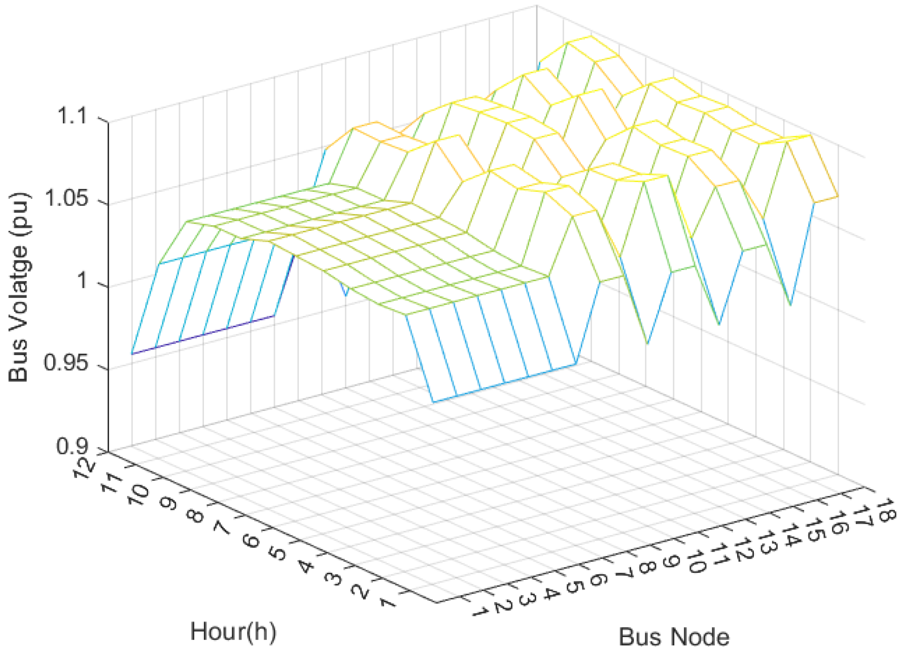
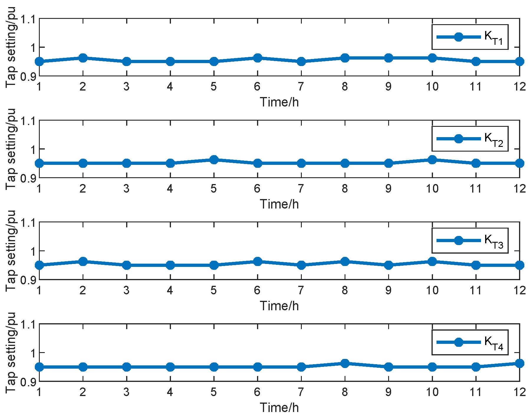
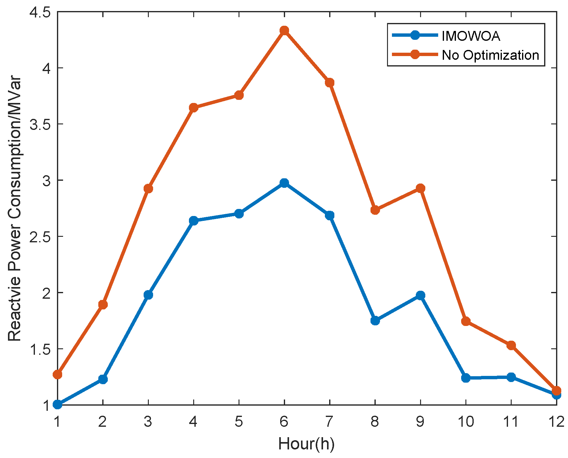
4.3.2. Case 2: Optimal Power Flow Optimization Under Fixed Voyage

In this case, we consider the optimal power flow optimization for HESPS under a fixed-voyage condition, where the number of populations of the algorithm is set to 100, the number of iterations is set to 700, and the rest of the parameters are set the same as in case 1. By using the trained WOA-CNN-LSTM attack and recovery model, the corrected data are obtained, as shown in Figure 8. By using Algorithm 1, the corresponding Pareto frontier and results of active power optimization per hour under MOGWO, MOWOA, and IMOWOA can be obtained, as shown in Figure 9 and Figure 10. The comparative results of costs, active power losses, and carbon emissions obtained by different algorithms are shown in Table 3, Table 4 and Table 5.

Obviously, Figure 9 and Figure 10 indicate that the proposed optimization algorithm based on IMOWOA outperforms other algorithms (MOGWO and MOWOA). That is to say, the developed algorithm can find the optimal solution set to achieve the goals of minimizing operating costs and minimizing active power loss.

It can be seen from

Table 10. Comparison of optimization results in case 2.

Evaluation Indicator	Cost ($)		Power Loss (MW)		CO2 Emission (kg)
	Value	Optimized Proportion	Value	Optimized Proportion	Value	Optimized Proportion
No optimization	52,408.89		2.1073		55,393.34
MOWOA	48,503.55	7.45%	1.6090	23.65%	51,352.51	7.29%
MOGWO	48,550.13	7.36%	1.6090	23.65%	51,858.39	6.38%
IMOWOA	47,475.46	9.41%	1.4894	29.32%	50,443.24	8.94%

that compared with the ship power system without optimization, the cost, power loss, and carbon emissions of the ship power system optimized by MOWOA, MOGWO, and IMOWOA are significantly reduced, and the optimization results can meet the EEOI constraint, keeping the EEOI indicator below the specified upper limit of 23 g CO₂/tn. This indicates that it is necessary to further improve the performance of the algorithm, which can further reduce the operating cost, power loss, and carbon emissions of ships. Obviously, the table shows that the improved multi-objective whale algorithm proposed in this paper can obtain better optimization results. Comparing IMOWOA with MOWOA and MOGWO, it can be found that on the basis of the other two algorithms, IMOWOA can further optimize the operation cost, power loss, and carbon emissions of ships by at least 1.96%, 5.67%, and 1.77%, respectively. These results show that the algorithm proposed in this chapter can effectively solve the optimization problem of hybrid-energy ships. Figure 11, Figure 12, Figure 13, Figure 14 and Figure 15 respectively show the optimization results of hybrid-energy ships running at fixed voyage obtained by using the proposed algorithm, including the optimization results of node voltage, transformer, shunt var compensator, energy scheduling, and reactive power consumption.

It can be seen from Table 10 that in this case, the improved multi-objective whale algorithm proposed in this chapter can obtain better optimization results. By further comparing IMOWOA with MOWOA and MOGWO, it can be found that based on the two algorithms of MOWOA and MOGWO, IMOWOA can further optimize the operation cost, power loss, and carbon emissions of ships by at least 2.86%, 3.70%, and 3.40%, respectively. These results show that the algorithm proposed in this paper can effectively solve the joint optimization problem of optimal power flow and speed of hybrid-energy ships.

In addition, Table 10 shows the results of voyage optimization. Compared with case 2 under fixed voyage, it can be seen that the cost and carbon dioxide emissions can be further reduced by 0.88% and 1.39%, respectively, through the joint optimization of the optimal power flow and speed of the ship.

As shown in Figure 11, it can be seen that the voltage of each node after optimization meets the security constraints. Compared with the voltage before optimization shown in Figure 16, the optimized voltage can be maintained at a higher level, which helps to reduce the loss of active power and prevent the system voltage from being too low. Finally, as shown in Figure 15, the optimized reactive power consumption is significantly reduced, thus ensuring voltage safety and reducing the active power loss of the system. To summarize, the proposed algorithm shows excellent effectiveness in solving the optimal power flow optimization problem of fixed navigation ships, and effectively reduces the cost, active power loss, and carbon emissions.

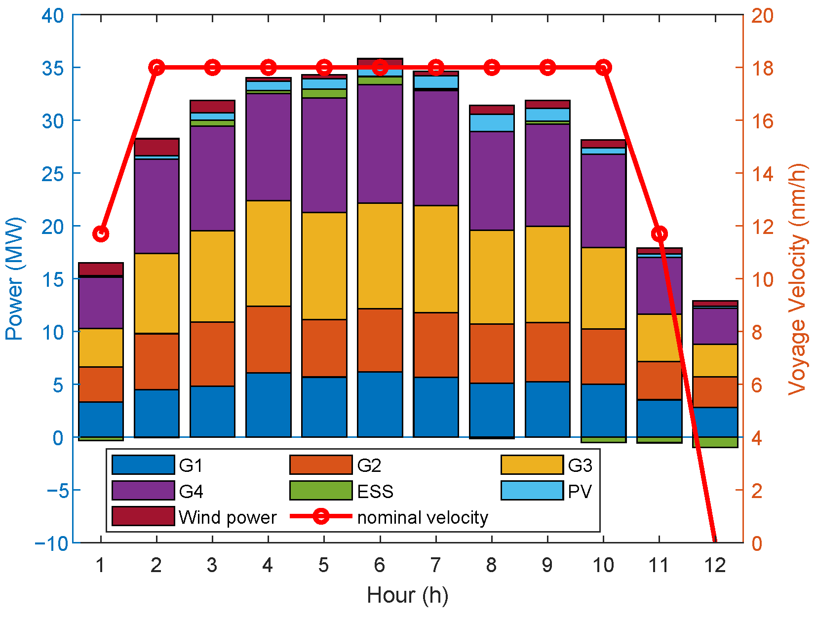
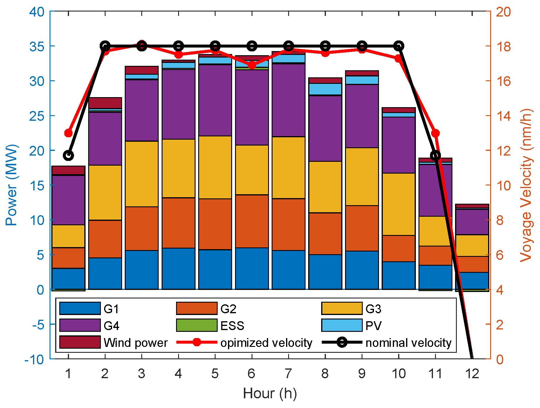
4.3.3. Case 3: Joint Optimization of Voyage and the Optimal Power Flow for HESPS

In this case, we consider the optimal power flow optimization for HESPS under a fixed-voyage condition, where the number of populations of the algorithm is set to 100, the number of iterations is set to 700, and the rest of the parameters are set the same as in case 1. By applying different algorithms, a comparison of Pareto frontier solution sets and the results of active power loss optimization per hour can be obtained, as shown in Figure 17 and Figure 18. The comparison results of cost, power loss, and carbon dioxide emission are also obtained, as shown in

Table 11. Comparison of optimization results in case 3.

Evaluation Indicator	Cost (USD)		Power Loss (MW)		CO2 Emission (kg)
	Value	Optimized Proportion	Value	Optimized Proportion	Value	Optimized Proportion
No optimization	52,408.89		2.1073		55,393.34
MOWOA	48,775.16	6.93%	1.5804	25.00%	51,627.78	6.80%
MOGWO	49,307.03	7.36%	1.6849	20.04%	52,125.60	5.90%
Improved NSGA-II	48,126.68	8.17%	1.5627	25.8%	51,087.16	7.77%
IMOWOA	47,054.75	10.22%	1.5026	28.70%	49,744.14	10.20%

.

The simulation results in Figure 17 and Figure 18 show that the proposed algorithm is also superior to the other two algorithms in solving the optimal scheduling problem of hybrid-energy ships under this working condition.

It can be seen from Table 11 that in this case, the improved multi-objective whale algorithm proposed in this chapter can obtain better optimization results. By further comparing IMOWOA with MOWOA and MOGWO, it can be found that based on the two algorithms of MOWOA and MOGWO, IMOWOA can further optimize the operation cost, power loss, and carbon emissions of ships by at least 2.86%, 3.70%, and 3.40%, respectively. These results show that the algorithm proposed in this paper can effectively solve the joint optimization problem of optimal power flow and speed of hybrid-energy ship.

In addition,

Table 12. The voyage optimization results for hybrid-energy ship using the proposed algorithm.

Evaluation Indicator	Cost ($)		CO2 Emission (kg)
	Value	Optimized Proportion	Value	Optimized Proportion
Fixed voyage (case 2)	$\mathrm{47,475.46}$		$\mathrm{50,443.24}$
Voyage optimization (case 3)	47,054.75	0.88%	49,744.14	1.39%

shows the results of voyage optimization. Compared with case 2 under fixed voyage, it can be seen that the cost and carbon dioxide emissions can be further reduced by 0.88% and 1.39%, respectively, through the joint optimization of the optimal power flow and speed of the ship.

In this case, Figure 19, Figure 20, Figure 21, Figure 22, Figure 23 and Figure 24 respectively show the joint optimization results of optimal power flow and voyage for hybrid-energy ship obtained by using the proposed algorithm, including the optimization results of node voltage, transformer, voyage, shunt var compensator, energy scheduling, and reactive power consumption.

According to Figure 20, the optimized voltage can be maintained in a safe range and at a high level. At the same time, Figure 24 shows that after optimization, the reactive power consumption of the system is reduced, which can reduce the active power loss of the system and ensure the normal operation of the system.

In summary, the simulation results from cases 1, 2, and 3 validate the optimization performance of the proposed Algorithm 1. Case 1 exhibits superior optimization performance compared to existing algorithms. Cases 2 and 3 demonstrate that Algorithm 1 enables one to effectively solve the joint optimization problem of optimal power flow and voyage to reduce operating costs, power loss, and carbon dioxide emissions. Furthermore, case 3 illustrates that the joint optimization of voyage and optimal power flow can further decrease operational costs and carbon dioxide emissions in HESPS when compared to case 2.

5. Conclusions and Future Works

This paper develops a secure two-stage optimization scheduling framework under FDIAs for HESPS, encompassing both the offline training phase and the online scheduling stage. The proposed model facilitates the detection and rectification of abnormalities in sensor data through the implementation of the WOA-CNN-LSTM model, thereby ensuring efficient follow-up scheduling. Additionally, an optimization strategy based on the IMOWOA is employed during the scheduling stage to address optimal power flow and joint optimization for hybrid ships, resulting in reduced operational costs, power loss, and carbon dioxide emissions. The specific conclusions are as follows: (1) A detection and recovery model for abnormal sensor data based on WOA-CNN-LSTM is established to enhance the safety of the ship scheduling process. (2) Leveraging the results from data detection and recovery, the IMOWA-based optimization strategy is utilized to optimize the scheduling of hybrid electric ships, achieving reductions in operating costs, power consumption, and carbon dioxide emissions by at least 1.96%, 5.67%, and 1.65%, respectively, compared to existing algorithms. (3) By coordinating the optimization of voyage planning with optimal power flow for hybrid-energy ships, further reductions in operation costs and carbon dioxide emissions of 0.88% and 1.39%, respectively, are attained.

Although the proposed method can address the problem of optimal scheduling for hybrid-energy ships under FDIAs, the model and algorithm presented in this paper still have certain limitations. The proposed detection model is primarily focused on identifying a single type of abnormal data, and its performance in recognizing different types of abnormal data is not satisfactory. The recovery model lacks sufficient capability to restore complex unknown data. The proposed scheduling algorithm is not effective in handling high-dimensional optimal scheduling problems. These issues will be addressed in future work, with a focus on the following aspects: enhancing the detection model’s ability to identify various types of abnormal data; improving the learning and recovery capabilities of the recovery model for complex unknown data; enhancing the proposed optimization algorithm’s ability to solve high-dimensional optimization scheduling problems; and considering the algorithm computing overhead and running time

References

1. Han, Y.; Ma, W.; Ma, D. Green maritime: An improved quantum genetic algorithm-based ship speed optimization method considering various emission reduction regulations and strategies. J. Clean. Prod. 2023, 385, 135814. [Google Scholar] [CrossRef]
2. Wang, H.; Lang, X.; Mao, W. Voyage optimization combining genetic algorithm and dynamic programming for fuel/emissions reduction. Transp. Res. Part D Transp. Environ. 2021, 90, 102670. [Google Scholar] [CrossRef]
3. RESOLUTION MEPC. Amendments to the annex of the protocol of 1997 to amend the international convention for the prevention of pollution from ships, 1973, as modified by the protocol of 1978 relating thereto. Amend. MARPOL Annex VI MEPC 2011, 70, 18. [Google Scholar]
4. Fan, A.; Li, Y.; Liu, H.; Yang, L.; Tian, Z.; Li, Y.; Vladimir, N. Development trend and hotspot analysis of ship energy management. J. Clean. Prod. 2023, 389, 135899. [Google Scholar] [CrossRef]
5. He, Y.; Mendis, G.J.; Wei, J. Real-time detection of false data injection attacks in smart grid: A deep learning-based intelligent mechanism. IEEE Trans. Smart Grid 2017, 8, 2505–2516. [Google Scholar] [CrossRef]
6. James, J.; Hou, Y.; Li, V.O. Online false data injection attack detection with wavelet transform and deep neural networks. IEEE Trans. Ind. Inform. 2018, 14, 3271–3280. [Google Scholar]
7. Zhang, G.; Li, J.; Bamisile, O.; Cai, D.; Hu, W.; Huang, Q. Spatio-temporal correlation-based false data injection attack detection using deep convolutional neural network. IEEE Trans. Smart Grid 2021, 13, 750–761. [Google Scholar] [CrossRef]
8. Wang, S.; Bi, S.; Zhang, Y.-J.A. Locational detection of the false data injection attack in a smart grid: A multilabel classification approach. IEEE Internet Things J. 2020, 7, 8218–8227. [Google Scholar] [CrossRef]
9. Mohammadpourfard, M.; Khalili, A.; Genc, I.; Konstantinou, C. Cyber-resilient smart cities: Detection of malicious attacks in smart grids. Sustain. Cities Soc. 2021, 75, 103116. [Google Scholar] [CrossRef]
10. Gao, X.; Yang, X.; Meng, L.; Wang, S. Fast economic dispatch with false data injection attack in electricity-gas cyber–physical system: A data-driven approach. ISA Trans. 2023, 137, 13–22. [Google Scholar] [CrossRef]
11. Chen, H.; Wu, H.; Kan, T.; Zhang, J.; Li, H. Low-carbon economic dispatch of integrated energy system containing electric hydrogen production based on vmd-gru short-term wind power prediction. Int. J. Electr. Power Energy Syst. 2023, 154, 109420. [Google Scholar] [CrossRef]
12. Vu, B.H.; Chung, I.-Y. Optimal generation scheduling and operating reserve management for pv generation using rnn-based forecasting models for stand-alone microgrids. Renew. Energy 2022, 195, 1137–1154. [Google Scholar] [CrossRef]
13. Wen, L.; Zhou, K.; Yang, S.; Lu, X. Optimal load dispatch of community microgrid with deep learning based solar power and load forecasting. Energy 2019, 171, 1053–1065. [Google Scholar] [CrossRef]
14. Yu, M.; Niu, D.; Wang, K.; Du, R.; Yu, X.; Sun, L.; Wang, F. Short-term photovoltaic power point-interval forecasting based on double-layer decomposition and woa-bilstm-attention and considering weather classification. Energy 2023, 275, 127348. [Google Scholar] [CrossRef]
15. Hein, K.; Xu, Y.; Wilson, G.; Gupta, A.K. Coordinated optimal voyage planning and energy management of all-electric ship with hybrid energy storage system. IEEE Trans. Power Syst. 2020, 36, 2355–2365. [Google Scholar] [CrossRef]
16. Zhang, Y.; Shan, Q.; Teng, F.; Li, T. Coordinated energy management scheme for ship-harbour energy system based on economic optimal scheduling. In Proceedings of the 2021 International Conference on Security, Pattern Analysis, and Cybernetics (SPAC), Chengdu, China, 18–20 June 2021; pp. 81–86. [Google Scholar]
17. Chen, G.; Liu, D.; Yan, L. Coordinated scheduling and optimal control of all-electric ship energy system based on mixed logical dynamic method. In Proceedings of the 8th Renewable Power Generation Conference (RPG 2019), IET, Shanghai, China, 24–25 October 2019; pp. 1–7. [Google Scholar]
18. Huang, Y.; Lan, H.; Hong, Y.-Y.; Wen, S.; Fang, S. Joint voyage scheduling and economic dispatch for all-electric ships with virtual energy storage systems. Energy 2020, 190, 116268. [Google Scholar] [CrossRef]
19. Du, W.; Li, Y.; Shi, J.; Sun, B.; Wang, C.; Zhu, B. Applying an improved particle swarm optimization algorithm to ship energy saving. Energy 2023, 263, 126080. [Google Scholar] [CrossRef]
20. Fang, S.; Xu, Y. Multi-objective robust energy management for all-electric shipboard microgrid under uncertain wind and wave. Int. J. Electr. Power Energy Syst. 2020, 117, 105600. [Google Scholar] [CrossRef]
21. Li, Z.; Xu, Y.; Wu, L.; Zheng, X. A risk-averse adaptively stochastic optimization method for multi-energy ship operation under diverse uncertainties. IEEE Trans. Power Syst. 2020, 36, 2149–2161. [Google Scholar] [CrossRef]
22. Xu, L.; Wen, Y.; Luo, X.; Lu, Z.; Guan, X. A modified power management algorithm with energy efficiency and ghg emissions limitation for hybrid power ship system. Appl. Energy 2022, 317, 119114. [Google Scholar] [CrossRef]
23. Li, Z.; Xu, Y.; Fang, S.; Wang, Y.; Zheng, X. Multiobjective coordinated energy dispatch and voyage scheduling for a multienergy ship microgrid. IEEE Trans. Ind. Appl. 2019, 56, 989–999. [Google Scholar] [CrossRef]
24. Wang, X.; Zhu, H.; Luo, X.; Chang, S.; Guan, X. A novel optimal dispatch strategy for hybrid energy ship power system based on the improved nsga-ii algorithm. Electr. Power Syst. Res. 2024, 232, 110385. [Google Scholar] [CrossRef]
25. Baldwin, T.L.; Lewis, S.A. Distribution load flow methods for shipboard power systems. IEEE Trans. Ind. Appl. 2004, 40, 1183–1190. [Google Scholar] [CrossRef]
26. Huang, Y.; Lan, H.; Hong, Y.-Y.; Wen, S.; Yin, H. Optimal generation scheduling for a deep-water semi-submersible drilling platform with uncertain renewable power generation and loads. Energy 2019, 181, 897–907. [Google Scholar] [CrossRef]
27. Zhu, J.; Hu, W.; Xu, X.; Liu, H.; Pan, L.; Fan, H.; Zhang, Z.; Chen, Z. Optimal scheduling of a wind energy dominated distribution network via a deep reinforcement learning approach. Renew. Energy 2022, 201, 792–801. [Google Scholar] [CrossRef]
28. He, Y.; Gao, Q.; Jin, Y.; Liu, F. Short-term photovoltaic power forecasting method based on convolutional neural network. Energy Rep. 2022, 8, 54–62. [Google Scholar] [CrossRef]
29. Houran, M.A.; Bukhari, S.M.S.; Zafar, M.H.; Mansoor, M.; Chen, W. Coa-cnn-lstm: Coati optimization algorithm-based hybrid deep learning model for pv/wind power forecasting in smart grid applications. Appl. Energy 2023, 349, 121638. [Google Scholar] [CrossRef]
30. Wang, X.; Wang, L.; Li, H.; Guo, Y. An improved whale optimization algorithm for global optimization and realized volatility prediction. Alex. Eng. J. 2023, 77, 2935–2969. [Google Scholar] [CrossRef]
31. Meng, A.-B.; Chen, Y.-C.; Yin, H.; Chen, S.-Z. Crisscross optimization algorithm and its application. Knowl.-Based Syst. 2014, 67, 218–229. [Google Scholar] [CrossRef]
32. Wang, W.L.; Li, W.K.; Wang, Z.; Li, L. Opposition-based multi-objective whale optimization algorithm with global grid ranking. Neurocomputing 2019, 341, 41–59. [Google Scholar] [CrossRef]
33. Zeng, N.; Song, D.; Li, H.; You, Y.; Liu, Y.; Alsaadi, F.E. A competitive mechanism integrated multi-objective whale optimization algorithm with differential evolution. Neurocomputing 2021, 432, 170–182. [Google Scholar] [CrossRef]
34. Li, M.; Xu, G.; Lai, Q.; Chen, J. A chaotic strategy-based quadratic opposition-based learning adaptive variable-speed whale optimization algorithm. Math. Comput. Simul. 2022, 193, 71–99. [Google Scholar] [CrossRef]
35. Huang, K.; Li, W.; Gao, F. Barabási-albert model-enhanced genetic algorithm for optimizing LGBM in ship power grid fault diagnosis. Measurement 2025, 249, 116954. [Google Scholar] [CrossRef]
36. Ma, L.; Zhang, P.; Sun, F.; Fang, J.; Zhang, C.; Xu, X. Mechanical Fault Diagnosis of High-Voltage Circuit Breakers Based on IPSO-VMD and KFCM-SVM. IEEJ Trans. Electr. Electron. Eng. 2025. [Google Scholar] [CrossRef]
37. Arazi, A.; Shapira, E.; Reichart, R. TabSTAR: A Foundation Tabular Model with Semantically Target-Aware Representations. In Proceedings of the AAAI Conference on Artificial Intelligence, Virtual, 19–21 May 2021; Volume 35. [Google Scholar]
38. Li, X.; Chen, H.; Xie, F.; Cao, C.; Wang, S.; Shuai, C. Hybrid Model of Multiple Echo State Network Integrated by Evidence Fusion for Fault Diagnosis of a High-Voltage Circuit Breaker. IEEE Trans. Consum. Electron. 2024, 70, 5269–5277. [Google Scholar] [CrossRef]
39. Mirjalili, S.; Saremi, S.; Mirjalili, S.M.; Coelho, L.D.S. Multi-objective grey wolf optimizer: A novel algorithm for multi-criterion optimization. Expert Syst. Appl. 2016, 47, 106–119. [Google Scholar] [CrossRef]
40. Kumawat, I.R.; Nanda, S.J.; Maddila, R.K. Multi-objective whale optimization. In Proceedings of the Tencon 2017—2017 IEEE Region 10 Conference, Penang, Malaysia, 5–8 November 2017; Volume 1, pp. 2747–2752. [Google Scholar]
Figure 1. The structure of the hybrid-energy ship.
Electricity 06 00038 g001
Figure 2. The detection and recovery framework for hybrid-energy ship systems under abnormal data.
Electricity 06 00038 g002
Figure 3. The structure of the CNN model.
Electricity 06 00038 g003
Figure 4. The structure of the LSTM.
Electricity 06 00038 g004
Figure 5. Comparison results of false data detection under different detection models.
Electricity 06 00038 g005
Figure 6. Comparison results of data recovery based on WOA-CNN-LSTM prediction model.
Electricity 06 00038 g006
Figure 7. Test results under different test functions: (a) test result of ZDT1; (b) test result of ZDT2; (c) test result of ZDT3.
Electricity 06 00038 g007
Figure 8. Corrected results based on WOA-CNN-LSTM attack detection and recovery model.
Electricity 06 00038 g008
Figure 9. Comparison result of Pareto frontier under different algorithms in case 2.
Electricity 06 00038 g009
Figure 10. Comparison of the power loss optimization results under different algorithms.
Electricity 06 00038 g010
Figure 11. The voltage optimization results under Algorithm 1 in case 2 (The line color represents the surface height (Z-axis value), corresponding to the magnitude of the voltage amplitude. By default, MATLAB uses a color gradient where low Z-values are rendered in blue (cool tones) and high Z-values are displayed in yellow or red (warm tones)).
Electricity 06 00038 g011
Figure 12. The transformer tap setting results under Algorithm 1 in case 2.
Electricity 06 00038 g012
Figure 13. The power optimization results under Algorithm 1 in case 2.
Electricity 06 00038 g013
Figure 14. The shunt var compensator output results under Algorithm 1 in case 2.
Electricity 06 00038 g014
Figure 15. The reactive power consumption optimization results under Algorithm 1 in case 2.
Electricity 06 00038 g015
Figure 16. The bus voltage before optimization. (The line color represents the surface height (Z-axis value), corresponding to the magnitude of the voltage amplitude. By default, MATLAB uses a color gradient where low Z-values are rendered in blue (cool tones) and high Z-values are displayed in yellow or red (warm tones)).
Electricity 06 00038 g016
Figure 17. Comparison result of Pareto frontier under three algorithms in case 3.
Electricity 06 00038 g017
Figure 18. The active power loss optimization results under Algorithm 1 in case 3.
Electricity 06 00038 g018
Figure 19. The shunt var compensator output optimization results under Algorithm 1 in case 3.
Electricity 06 00038 g019
Figure 20. The node voltage optimization results under Algorithm 1 in case 3 (The line color represents the surface height (Z-axis value), corresponding to the magnitude of the voltage amplitude. By default, MATLAB uses a color gradient where low Z-values are rendered in blue (cool tones) and high Z-values are displayed in yellow or red (warm tones)).
Electricity 06 00038 g020
Figure 21. The transformer tap setting optimization results under Algorithm 1 in case 3.
Electricity 06 00038 g021
Figure 22. The voyage optimization results under Algorithm 1 in case 3.
Electricity 06 00038 g022
Figure 23. The power optimization results under Algorithm 1 in case 3.
Electricity 06 00038 g023
Figure 24. The reactive power consumption optimization results under Algorithm 1 in case 3.
Electricity 06 00038 g024