Heuristic-Based Scheduling of BESS for Multi-Community Large-Scale Active Distribution Network

Abstract

The integration of battery energy storage systems (BESSs) within active distribution networks (ADNs) entails optimized day-ahead charge/discharge scheduling to achieve effective peak shaving.The primary objective is to reduce peak demand and mitigate power deviations caused by intermittent photovoltaic (PV) output. Quasi-static time-series (QSTS) co-simulations for determining optimal heuristic solutions at each time interval are computationally intensive, particularly for large-scale systems. To address this, a two-stage intelligent BESS scheduling approach implemented in a MATLAB–OpenDSS environment with parallel processing is proposed in this paper. In the first stage, a rule-based decision tree generates initial charge/discharge setpoints for community BESS units. These setpoints are refined in the second stage using an optimization algorithm aimed at minimizing community net load power deviations and reducing peak demand. By assigning each ADN community to a dedicated CPU core, the proposed approach utilizes parallel processing to significantly reduce the execution time. Performance evaluations on an IEEE 8500-node test feeder demonstrate that the approach enhances peak shaving while reducing QSTS co-simulation execution time, utility peak demand, distribution network losses, and point of interconnection (POI) nodal voltage deviations. In addition, the use of smart inverter functions improves BESS operations by mitigating voltage violations and active power curtailment, thereby increasing the amount of energy shaved during peak demand periods.

1. Introduction

1.1. Motivation

In recent years, the power grid has been undergoing modernization through widespread deployment of smart grid technologies including renewable energy systems (RESs) and advanced sensing devices across its distribution networks (DNs). The large volumes of granular data from smart meters can be processed to generate valuable insights about the DN spatiotemporal electric conditions and characterize modern load behavior for participation in demand-side management and demand response programs, and help develop operational planning strategies that can accommodate the increasing penetration of RESs in the DN while providing flexibility measures to the distribution system operator (DSO).

Operating an ADN, which is a DN with RES penetration, can be challenging, particularly due to high spatiotemporal load flow variations, i.e., nodal voltage fluctuations and bidirectional current flow. In fact, distributed and intermittent-nature photovoltaic (PV) systems’ power injections in a radial ADN can lead to static voltage violations and reverse power flow [1].

To address these issues, many utilities have begun integrating utility-scale battery energy storage systems (BESSs) at the community or microgrid level [2]. While each community BESS can operate independently, to reduce PV curtailment and maximize resource utilization, the operation of a BESS needs to be scheduled considering community load and PV as well as the external utility grid and DSO. With multiple PV-BESS communities, the BESS scheduling problem requires coordinated power management among communities to facilitate more effective power sharing between BESS units, improving state of charge (SoC) balancing, and avoiding oversized units [3].

Most BESS scheduling strategies do not scale well in large, multi-community ADNs due to computational complexity [4]. As the number of nodes and communities increases, determining the charge and discharge operations becomes a high-dimensional, time-sensitive problem [5]. This complexity is further intensified by solar irradiance and demand variability, and inverter-based control functions. Scalable and more computationally improved frameworks are required to optimally schedule BESS operations across several communities within an ADN, while considering the BESS energy or power applications [6].

1.2. Literature Review

BESS operation scheduling has been widely studied in both energy and power applications within DNs. Power-based applications are suitable for short-term services, including operating reserves and ancillary services such as primary voltage and frequency regulation. While BESS energy applications are suitable for long-term services with relatively slow charge/discharge rates, such as black-start, PV curtailment reduction, load balancing, energy arbitrage, and peak shaving [7]. The authors in [8] propose a peak load shaving algorithm developed for isolated microgrids using a hybrid PV–BESS system. The approach coordinated PV generation and BESS charge/discharge operations to address both midday and evening peaks. While the method shows effective load reduction and cost savings under real-world conditions, it focuses on energy dispatch and does not consider the dynamic role of inverter-based control functions in regulating voltage or curtail peak output power. In [9], three BESS charge scheduling approaches are evaluated for real-world peak shaving applications: BESS slow charging based on a low utility setpoint, time-based charging based on periods of high PV and low energy cost, and fast charging irrespective of time and utility threshold. The authors conclude that while fast charging achieved the greatest bill reduction, it resulted in higher battery degradation due to increased charge/discharge cycles. Ideally, an optimal BESS charge/discharge operation strategy should consider battery lifetime in addition to the net load profile and electricity tariff rates. Similarly, Ref. [10] proposes a multi-objective function to minimize the costs associated with BESS operation and load fluctuations. A demand response scheme is incorporated for effective peak shaving and valley filling in the microgrid. In [11], a two-stage approach is developed to improve BESS peak shaving considering day-ahead net energy demand and battery operational limits. The first stage linearizes the power flow problem using a multivariate linear regression approach to obtain the DN variables. This linearization allows one to utilize a linear programming formulation in the second stage to determine the BESS charge/discharge setpoint at each time interval. The objective function in this stage is to minimize the maximum deviation of the new net demand from the average daily net demand. This leads to the optimal peak-shaving setpoint. However, such centralized and sequential scheduling methods become computationally intensive in large-scale networks. Considering the computational complexity of the aforementioned approaches, optimal multi-community BESS scheduling in large-scale multi-energy DNs—often consisting of thousands of electrical nodes—requires parallel processing techniques to distribute the computational workload among various hardware processor cores [12,13].

1.3. Contributions

However, existing strategies often lack scalability for interconnected, utility-scale community ADNs. They separate BESS scheduling and smart inverter-based control. The challenge lies in developing a scalable, integrated framework utilizing OpenDSS parallel processing feature to optimize BESS scheduling across multiple ADN communities while concurrently managing SoC balancing and power sharing, and mitigating fluctuations arising from intermittent SIR and demand variability [14]. Such a framework would provide significant benefits to utility operational planning by enabling coordinated control of DERs. This study adopts the perspective of a utility-operated DN, where the utility can observe BESS scheduling across multiple communities while solar irradiance demand is not controlled.

The main contributions of this paper are as follows:

• Development of a Two-Stage Optimal BESS Scheduling Problem. A two-stage optimization approach is developed, combining a rule-based decision tree method to determine initial charge/discharge setpoints for community BESS units, while these setpoints are refined in the second stage using an optimization algorithm aimed at minimizing adjacent community net load power deviations and reducing peak demand.
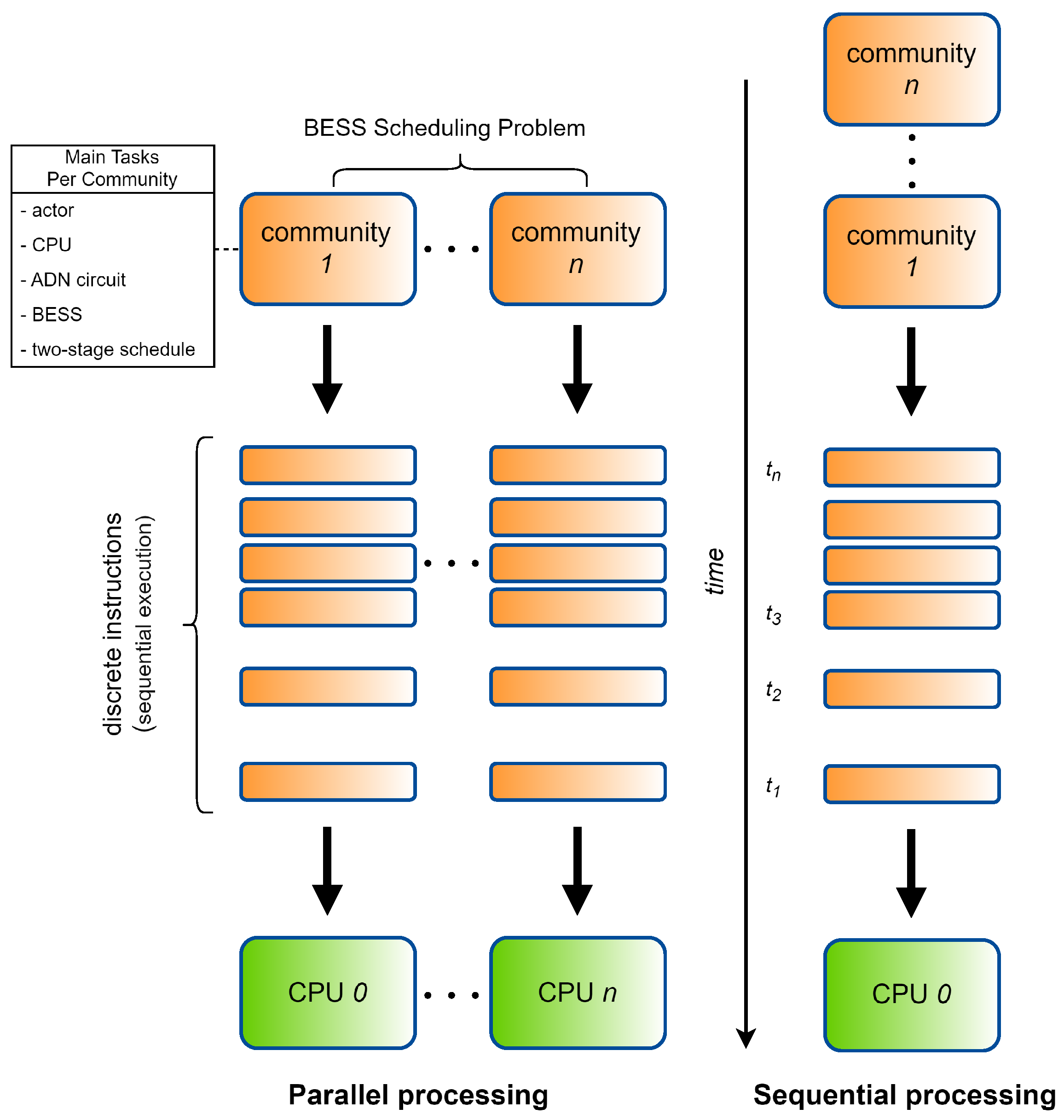
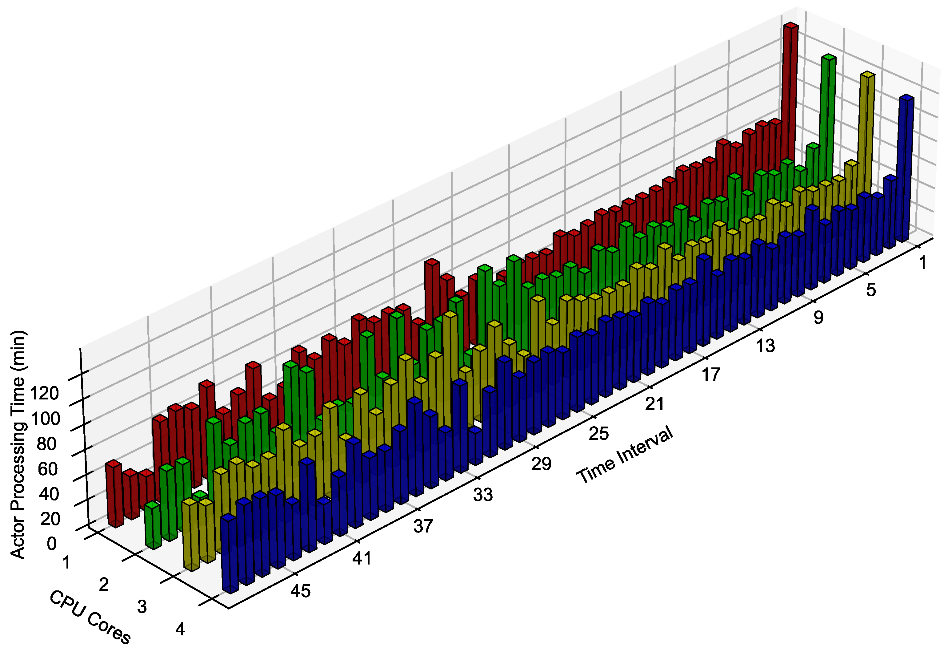
• Parallel Processing for Multi-Community BESS Scheduling. An OpenDSS parallel machine (PM) is utilized, with each workstation CPU core being dedicated to executing the two-stage BESS scheduling problem for individual communities, leveraging parallel processing for computational efficiency in large-scale ADNs, thereby distributing computational workload across CPU cores, for iterative quasi-static time-series heuristic simulation for utility-scale DN.
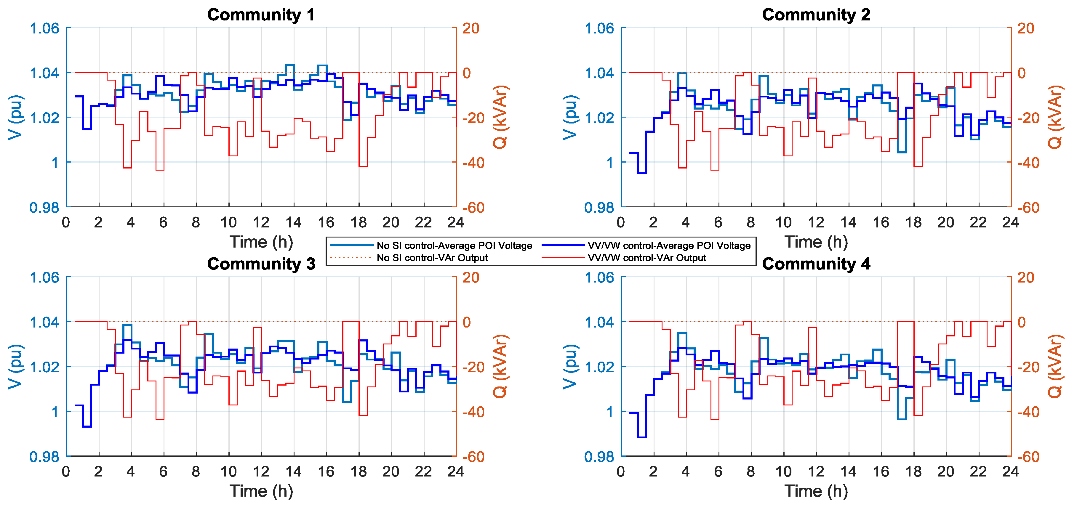
• Smart inverter functionalities are assessed to further improve BESS operations by mitigating voltage violations through the combined use of the volt–VAr and volt–watt control functions. A control setpoint curve is implemented, enabling coordinated reactive power support based on nodal voltage measurements at the point of interconnection. This combined control strategy improves the nodal voltage regulation.

The rest of the paper is organized as follows: Section 2 describes the ADN components modeling and formulates the BESS scheduling problem. In Section 3, the MATLAB–OpenDSS co-simulation environment and utilization of the parallel processing feature are detailed. Section 4 provides the case studies overview, simulation results, and discussions. Finally, the concluding remarks are given in Section 5.

2. Problem Formulation

The integration of BESS with distributed energy resources in active distribution networks (ADNs) is essential for ensuring grid reliability and optimizing energy usage. BESS scheduling for multiple communities in an ADN is a complex task due to each community’s varying energy demands and the need for efficient resource allocation [15]. This section formulates the BESS scheduling problem by defining its objectives, constraints, and variables. The goal is to develop a framework that ensures efficient energy distribution, minimizes the objective function, and enhances ADN reliability.

Effective energy scheduling of a BESS depends on an operational approach that utilizes historical day-ahead demand and the output from various distributed resources. This approach can significantly reduce peak demand and lower distribution system losses. To implement this approach, it is essential to calculate and communicate the charge/discharge power of the BESS at each time interval, which indicates the power to be absorbed or generated during each time interval.

This paper proposes a two-stage BESS scheduling approach that minimizes peak demand, reduces power deviations, and decreases energy losses across multiple communities in an ADN. Before detailing the optimization approach, we first explain the modeling of BESS within the ADN framework.

2.1. BESS Modeling

The BESS within an ADN manages power fluctuations from intermittent DERs to optimize energy usage. The BESS is connected to the grid at the point of interconnection (POI) via voltage source converters (VSCs). The power flow to and from the BESS is determined by its charge and discharge rates, and the state of charge (SoC), which is dynamically updated at each time step.

The optimization problem aims to determine the optimal scheduling of the BESS over M time intervals. The decision variable here is the active power value of the BESS, $P_k^{\mathit{BESS}}$, which is the amount of power that the system can charge or discharge during each interval k and can be expressed as:

$${\mathit{P}}^{\mathit{BESS}}=\left[\begin{array}{c}{P}_1^{\mathit{BESS}},P_2^{\mathit{BESS}},\dots ,P_k^{\mathit{BESS}},\dots ,P_M^{\mathit{BESS}}\end{array}\right]$$

(1)

A positive value of $P_k^{\mathit{BESS}}$ indicates the BESS is discharging and supplying power to the POI, while a negative value indicates the BESS is charging and acting as a load. When the value of $P_k^{\mathit{BESS}}$ is zero, the BESS is in an idling state. The SoC at the end of the time interval k, ${\mathit{SoC}}_k$, is calculated from the SoC of the previous interval, ${\mathit{SoC}}_{k-1}$ [16]. The change in SoC during the interval, $\Delta {\mathit{SoC}}_k$, is expressed as.

$${\mathit{SoC}}_k={\mathit{SoC}}_{k-1}+\Delta {\mathit{SoC}}_k$$

(2)

The change in SoC, $\Delta {\mathit{SoC}}_k$, accounts for charge/discharge efficiencies ($\xi$) and is defined in the following equation:

$$\Delta {\mathit{SoC}}_k={\displaystyle \frac{P_k^{\mathit{BESS}}·\xi ·{\eta }_{\mathit{inv}}·\Delta k}{B_{\mathit{kWh},\mathit{rated}}}}$$

(3)

The charge/discharge efficiency ($\xi$) can be expressed as:

$$\xi =\left\{\begin{array}{cc}{\eta }_{\mathit{chg}},\hfill & P_k^{\mathit{BESS}}<0,\hfill \\ {\displaystyle \frac{1}{{\eta }_{\mathit{dischg}}}},\hfill & P_k^{\mathit{BESS}}>0,\hfill \\ 0,\hfill & P_k^{\mathit{BESS}}=0\hfill \end{array}\right.$$

(4)

where ${\eta }_{\mathit{inv}}$ is the inverter efficiency, $B_{\mathit{kWh},\mathit{rated}}$ denotes the rated BESS capacity in kWh, and ${\eta }_{\mathit{chg}}$ and ${\eta }_{\mathit{dischg}}$ represent the charging and discharging efficiencies, respectively.

2.2. Smart Inverter Control Function

Co-located PV-BESS systems near community load centers can provide power quality services and enhance resilience during severe weather conditions, such as high cloud variability that impacts PV output power [17]. High variability in solar irradiance and varying load levels, especially under high PV penetration, can lead to power and voltage variations at the community’s POI [18]. This highlights the importance of advanced features that minimize these effects.

The IEEE 1547-2018 standard enables distributed energy resources to support grid functionalities through advanced features [19]. These features can be used by utilities to provide more reliable and resilient energy. One key advanced functionality of smart PV inverters is voltage support. The steady-state smart inverter voltage support is achieved by injecting or absorbing reactive power during undervoltage and overvoltage conditions near the POI’s normal operating voltage. This helps keep the POI voltage steady and boosts grid reliability.

This study also employs various smart inverter control modes to provide steady-state voltage support during undervoltage and overvoltage conditions caused by high levels of intermittent PV power, which impacts voltage quality in the distribution network. The control modes examined include Constant Power Factor (CPF), volt–VAr (VV), volt–watt (VW), and a combined volt–VAr/volt–watt (VV/VW) mode.

2.2.1. Constant Power Factor (CPF) Control Mode

The CPF mode operates by maintaining a fixed power factor regardless of voltage variations at the POI. The power factor, typically chosen by the utility, can be either leading (capacitive) or lagging (inductive), depending on the desired reactive power compensation. The inverter injects or absorbs reactive power accordingly to maintain the specified power factor (PF). The reactive power (Q) is linearly dependent on active power (P), defined as:

$$Q=P·tan\left(arccos\left(\mathrm{PF}\right)\right)$$

(5)

The apparent power (S) can be calculated as:

$$S=\sqrt{P^2+Q^2}$$

(6)

The CPF control mode effectively compensates for power fluctuations caused by changes in solar irradiance by dynamically adjusting reactive power (Q) to maintain the constant power factor (P).

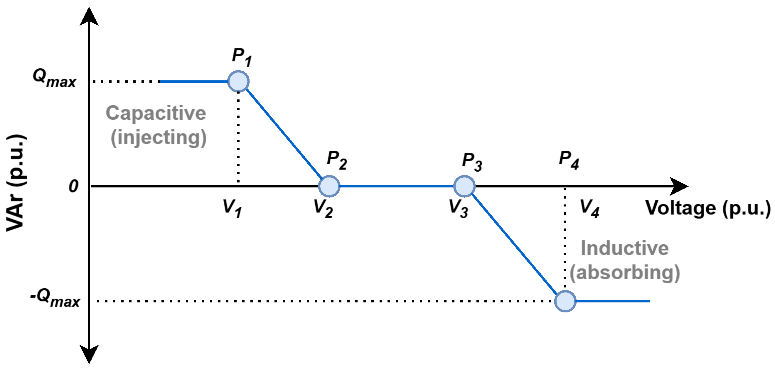
2.2.2. Volt–VAr (VV) Control Mode

The volt–VAr control mitigates voltage violations by injecting or absorbing reactive power according to the monitored voltage at the POI. The volt–VAr control curve, defined by voltage parameters $V_1$ to $V_4$, is illustrated in Figure 1. The reactive power capability of smart inverters is limited by their fixed apparent power capacity (kVA rating) [20]. The combined output of active power (P) and reactive power (Q) must remain within its capacity (S). The Q priority configuration ensures reactive power compensation to maintain voltage support, especially during voltage deviations.

The output reactive power to be injected/absorbed by the inverter in volt–VAr mode is expressed in the following equation.

$$Q=\left\{\begin{array}{cc}{Q}_{\max },\hfill & \mathrm{if}V\le V_1\hfill \\ Q_{\max }·{\displaystyle \frac{(V-V_2)}{(V_1-V_2)}},\hfill & \mathrm{if}{V}_1<V<V_2\hfill \\ 0,\hfill & \mathrm{if}{V}_2\le V\le V_3\hfill \\ -Q_{\max }·{\displaystyle \frac{(V-V_3)}{(V_4-V_3)}},\hfill & \mathrm{if}{V}_3<V<V_4\hfill \\ -Q_{\max },\hfill & \mathrm{if}V\ge V_4\hfill \end{array}\right.$$

(7)

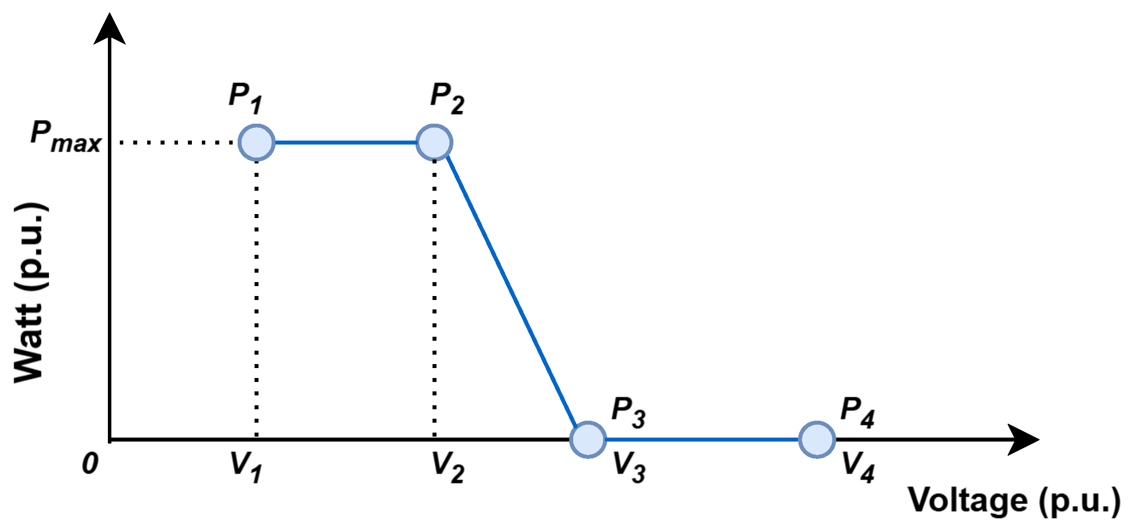
2.2.3. Volt–Watt (VW) Control Mode

This VW control mode limits the active power of the smart inverter by curtailing the generation when the voltage at the POI exceeds a specified threshold, thereby preventing voltage rise as seen in Figure 2 [21]. The following equation determines the total active power of the PV in volt–watt mode:

$$P=\left\{\begin{array}{cc}{P}_{\max },\hfill & \mathrm{if}V\le V_2\hfill \\ {\displaystyle \frac{(V-V_2)}{(V_3-V_2)}}·P_{\max },\hfill & \mathrm{if}{V}_2<V<V_3\hfill \\ 0,\hfill & \mathrm{if}V\ge V_3\hfill \end{array}\right.$$

(8)

The combined volt–VAr/volt–watt (VV/VW) control mode dynamically injects or absorbs reactive power to prevent voltage violations at the monitored nodes while curtailing active power to limit voltage rise. This dual approach maintains voltage safety at the point of interconnection by addressing both reactive and active power contributions to voltage variations, which is critical in a DN with high PV penetration where intermittent generation can challenge voltage regulation [22].

By utilizing the combined VV/VW advanced smart inverter function, the proposed two-stage BESS scheduling approach effectively mitigates voltage fluctuations and enhances power quality within the active distribution network. Specifically, the BESS injects or absorbs reactive power at the community point of interconnections to prevent voltage violations and curtails active power to limit voltage rise. This combined control, integrated with BESS scheduling, enables the achievement of an optimal operational schedule, ensuring adherence to power quality and grid standards.

2.3. BESS Scheduling Approach

2.3.1. Stage 1—Decision Tree Rule-Based Method

The decision tree rule-based method begins by comparing the net load demand ($D_k^d$) and available PV power output ($P_k^{PV}$) for each community at the point of interconnection (POI). Following a similar methodology as described in [8], Stage 1 determines the initial setpoint of the BESS. Additionally, the state of charge (SoC) value of each BESS, accessed against its predefined limits (${\mathrm{SoC}}_{min}$, ${\mathrm{SoC}}_{max}$) at time interval k, has been considered in the analysis. The stage ensures that each community’s BESS effectively utilizes the available PV power at the POI during charging operations. The rule-based statements established the decision variable’s setpoints, as outlined in (9).

$$P_k^{\mathit{BESS},n}=\left\{\begin{array}{cc}{P}_{A,\mathit{BESS}},\hfill & \mathrm{if}{P}_k^{\mathrm{PV}}>D_k^{\mathrm{d}}\&{\mathrm{SoC}}_{\mathit{BESS},n}<{\mathrm{SoC}}_{\max }\hfill \\ P_{B,\mathit{BESS}},\hfill & \mathrm{if}{P}_k^{\mathrm{PV}}\le D_k^{\mathrm{d}}\hfill \\ 0,\hfill & \mathrm{otherwise}(\mathrm{BESS}\mathrm{in}\mathrm{idling}\mathrm{mode})\hfill \end{array}\right.$$

(9)

where $P_{A,\mathit{BESS}}=D_k^{\mathrm{d}}+P_{\mathrm{k}}^{\mathrm{PV},\sup },P_{B,\mathit{BESS}}=D_k^{\mathrm{d}}$

At each time interval k, $P_k^{BESS}$ represents the BESS charging or discharging power. $P_k^{PV}$ and $D_k^d$ denote the PV output power and the forecasted day-ahead community demand at the BESS node, respectively. Additionally, $P_k^{PV,sup}$ refers to the surplus PV output power generated at each community’s POI when PV generation surpasses demand. The computed value of (9) from $P_k^{BESS}$ is then used as the input setpoint for the PSO algorithm in the subsequent stage.

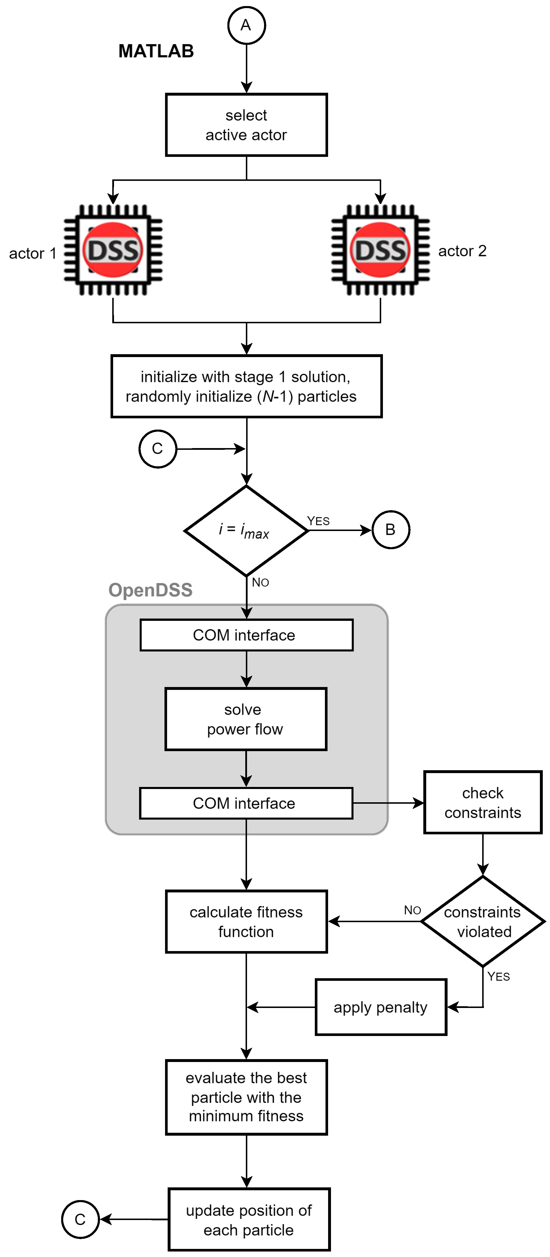
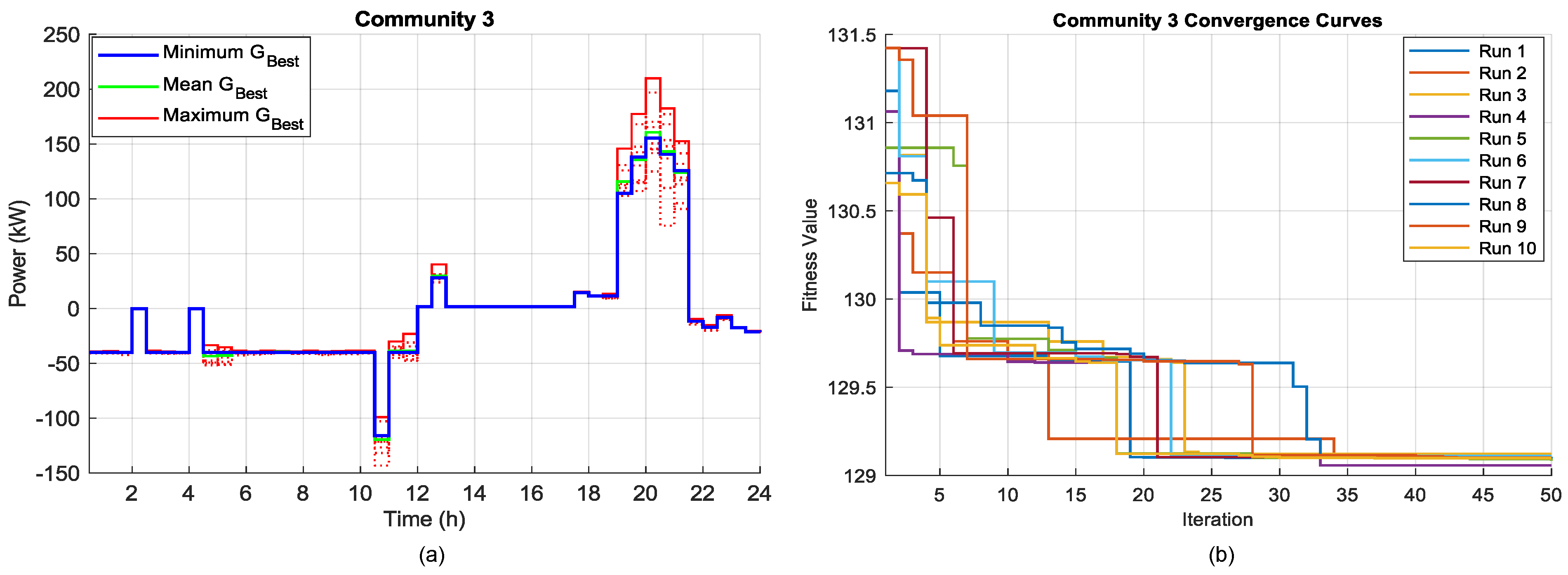
2.3.2. Stage 2—BESS Charge/Discharge Setpoint Optimization

In modern active distribution networks, the BESS plays a crucial role in enhancing grid reliability and optimizing energy flow. Effective management of BESS operations is essential for mitigating demand fluctuations and significant decreases in DN losses. The goal of the optimization problem is to determine the optimal charging and discharging setpoints for each community’s BESS within the active distribution network. The optimization aims to achieve peak shaving and valley filling, thereby reducing the net power demand from the DN and reducing peak load levels. Consequently, the decision variable in this optimization process is the amount of power that the BESS absorbs or discharges while adhering to power system and BESS operational constraints [11].

Power deviations in ADNs occur due to the intermittent output of PV systems, which are influenced by varying solar irradiance. The goal of the optimization is to minimize the maximum deviation between the new net demand and the daily average net demand at each community’s POI. By achieving this, the optimization yields a more stable and balanced demand profile, reduces peak demand, and fills demand valleys. The optimization problem can be expressed as follows:

$$\underset{P_k^{\mathit{BESS}}\forall k\in \{1,2,\dots ,M\},M=48}{min}{\Delta }_k$$

(10)

$${\Delta }_k=max\left|D_k^{\mathrm{net}}-D_{\mathrm{avg}}^{\mathrm{net}}\right|$$

(11)

$$D_k^{\mathrm{net}}=D_k^{\mathrm{d}}-P_k^{\mathrm{PV}}-P_k^{\mathit{BESS}}$$

(12)

$$D_{\mathrm{avg}}^{\mathrm{net}}={\displaystyle \frac{1}{M}}\sum _{k=1}^M{D}_k^{\mathrm{net}}$$

(13)

where ${\Delta }_k$ represents the maximum power deviation at each time interval k and serves as the objective function to be minimized. The variable M represents the total number of 30-minute time intervals during the day. The new net demand at each time interval is denoted as $D_k^{\mathrm{net}}$, while $D_{\mathrm{avg}}^{\mathrm{net}}$ is the average net demand for the day, which is derived from the day-ahead demand profile. The forecasted day-ahead demand at each time interval is given by $D_k^{\mathrm{d}}$. The output power from the PV system, $P_k^{\mathrm{PV}}$, is determined based on the PV array’s rated maximum power ($pmpp$), in kW, its temperature correction factor ($P{V}_{tcf}$), and the nominal SIR profile, ${\mathit{irrad}}_k$, at time interval k [23]. This relationship is expressed as:

$$P_k^{\mathrm{PV}}=\mathit{pmpp}·{\mathit{irrad}}_k·{\mathit{PV}}_{\mathit{tcf}}$$

(14)

2.4. Optimization Constraints

The optimization constraints for determining the optimal solution at each time interval for the objective function in (10) include both power system constraints and BESS operational constraints.

2.4.1. Power System Constraints

During the optimization process, load flow calculations are performed for each time interval k. Power system constraints guarantee that every nodal voltage ($V_k^{node}$) remains within ANSI limits [24] at each time interval. Additionally, the line current on each branch at each interval ($I_k^{line}$) must not exceed the maximum permissible line current capacity ($I_{max}^{line}$) as established in (16).

$$V_{\min }\le V_k^{\mathrm{node}}\le V_{\max },\forall k\in {\mathcal{N}}_B,k=1,2,\dots ,M$$

(15)

$$\left|I_k^{\mathrm{line}}\right|\le I_{\max }^{\mathrm{line}},\forall k\in {\mathcal{N}}_L,k=1,2,\dots ,M$$

(16)

where ${\mathcal{N}}_B$ and ${\mathcal{N}}_L$ are the sets of all nodes and lines in the distribution network, respectively. Equation (17) describes the equality constraints of active and reactive power balance that should be satisfied at each node.

$$\begin{array}{cc}\hfill P_{G_i}-P_{L_i}-V_i\sum _{j\in {\mathcal{N}}_B}{V}_j\left[G_{ij}cos({\theta }_i-{\theta }_j)+B_{ij}sin({\theta }_i-{\theta }_j)\right]& =0\hfill \\ \hfill Q_{G_i}-Q_{L_i}-V_i\sum _{j\in {\mathcal{N}}_B}{V}_j\left[G_{ij}sin({\theta }_i-{\theta }_j)-B_{ij}cos({\theta }_i-{\theta }_j)\right]& =0\hfill \end{array}$$

(17)

where $P_{Gi}$ and $P_{Li}$ are the generated and demand active power, and $Q_{Gi}$ and $Q_{Li}$ are the generated and demand reactive power, respectively. $V_i$ and $V_j$ represent the voltage magnitudes at buses i and j, ${\theta }_i$ and ${\theta }_j$ denote the voltage angles at buses i and j, and $G_{ij}$ and $B_{ij}$ correspond to the real and imaginary components of the $i{j}^{th}$ term in the bus admittance matrix.

2.4.2. BESS Operation Constraints

The BESS operation constraints considered in this paper include the maximum and minimum limits for both the charging and discharging BESS power, as well as the upper and lower bounds for the SoC of the battery energy storage system; these are detailed in (18) and (19).

$$-P_{\mathit{max}}^{\mathrm{Chg}}\le P_k^{\mathit{BESS}}\le P_{\mathit{max}}^{\mathrm{Dischg}}$$

(18)

$${\mathrm{SoC}}_{\min }\le {\mathrm{SoC}}_k\le {\mathrm{SoC}}_{\max }$$

(19)

where $P_{\mathit{max}}^{\mathit{Chg}}$ and $P_{\mathit{max}}^{\mathit{Dischg}}$ represent the maximum charging and discharging power of the BESS at each time interval k, respectively. The upper SoC limit ${\mathit{SoC}}_{\mathit{max}}$ is set to 100%, while the lower SoC limit ${\mathit{SoC}}_{\mathit{min}}$ is set at 15%. The SoC at time interval k is ${\mathit{SoC}}_{\mathit{k}}$. The minimum level serves as the battery’s reserve capacity; if the SoC falls below this level, the BESS switches to an idling state.

2.5. The Penalty Function

To ensure compliance with power system and BESS operational constraints, penalty functions are used to incorporate equality and inequality constraints into the optimization algorithm. The equality and inequality constraints, (15)–(19), are integrated into the optimization algorithm through the use of penalty functions. The penalty function evaluates the penalties associated with any violations of the power system or BESS operational constraints. If a violation is detected, the corresponding penalty is added to the objective function in (10). The penalty function is designed to penalize violations based on their magnitude, thereby guiding the optimization algorithm towards feasible and optimal solutions while minimizing constraint violations. The expressions for the penalty functions are.

$${\lambda }_{\left(\mathit{x}\right)}=\left\{\begin{array}{cc}{c}_{\mathit{p}},\hfill & \mathrm{if}\exists k:V_k^{\mathrm{node}}\ge V_{\min }\mathrm{and}{V}_k^{\mathrm{node}}\le V_{\max }\hfill \\ 0,\hfill & \mathrm{otherwise}\hfill \end{array}\right.$$

(20)

$$\begin{array}{cc}\hfill {\mathrm{\Lambda }}_{\left(\mathit{x}\right)}=\sum _{k=1}^M& \left(c_{\mathit{p}}·\left[max(0,V_{\min }-V_k^{\mathrm{node}})\right.\right.\hfill \\ \hfill & \left.\left.+max(0,-V_k^{\mathrm{node}}+V_{\max })\right]\right)\hfill \end{array}$$

(21)

$${\gamma }_{\left(\mathit{x}\right)}=\left\{\begin{array}{cc}{c}_{\mathit{p}},\hfill & \mathrm{if}\exists k:|I_{\mathrm{line}}|>I_{\max }^{\mathrm{line}}\hfill \\ 0,\hfill & \mathrm{otherwise}\hfill \end{array}\right.$$

(22)

$${\rho }_{\left(\mathit{x}\right)}=\left\{\begin{array}{cc}{c}_{\mathit{p}},\hfill & \mathrm{if}\exists k:{\mathrm{SoC}}_k<{\mathrm{SoC}}_{\min }\mathrm{or}{\mathrm{SoC}}_k>{\mathrm{SoC}}_{\max }\hfill \\ 0,\hfill & \mathrm{if}\exists k:{\mathit{SoC}}_{\mathit{min}}\le {\mathit{SoC}}_k\le {\mathit{SoC}}_{\mathit{max}}\hfill \end{array}\right.$$

(23)

$${\psi }_{\left(\mathit{x}\right)}=\left\{\begin{array}{cc}{c}_{\mathit{p}},\hfill & \mathrm{if}\exists k:P_k^{\mathit{BESS}}<-P_{\mathit{max}}^{\mathrm{Chg}}\mathrm{or}{P}_k^{\mathit{BESS}}>P_{\mathit{max}}^{\mathrm{Dischg}}\hfill \\ 0,\hfill & \mathrm{otherwise}\hfill \end{array}\right.$$

(24)

where $c_{\mathit{p}}$ represents a numerical value assigned to each violation incurred to quantify the severity of the penalty associated with that particular violation. The term ${\lambda }_{\left(\mathit{x}\right)}$ refers to the penalty applied for individual nodal voltage violations, while ${\mathrm{\Lambda }}_{\left(\mathit{x}\right)}$ signifies the overall penalty resulting from voltage violations across the entire network. ${\gamma }_{\left(\mathit{x}\right)}$ indicates the penalty incurred due to overcurrent occurrences in lines or branches, and ${\rho }_{\left(\mathit{x}\right)}$ is the penalty imposed for violations of SoC limits during time interval k. ${\psi }_{\left(\mathit{x}\right)}$ is the penalty associated with violations of the BESS charge and discharge power limits. The decision variable x corresponds to the BESS charge/discharge power and it is determined for every time interval k$\in \{1,2,3,\dots ,M\}$ and M = 48.

Equations (20)–(24) are important for the optimization algorithm as they guarantee the safe and efficient operation of the system by adhering to the operational constraints of the power systems and battery energy storage system within the ADN. The penalties guide the optimization process to achieve an optimal charge/discharge schedule. The overall penalty function, $g_{\left(\mathit{x}\right)}$, is formulated as:

$$g_{\left(\mathit{x}\right)}={\mathrm{\Lambda }}_{\left(\mathit{x}\right)}+{\gamma }_{\left(\mathit{x}\right)}+{\rho }_{\left(\mathit{x}\right)}+{\psi }_{\left(\mathit{x}\right)}$$

(25)

Using (10) and (25), the overall objective function is expressed as.

$${\Delta }_k=max\left|D_k^{\mathrm{net}}-D_{\mathrm{avg}}^{\mathrm{net}}\right|+g_{\left(\mathit{x}\right)}$$

(26)

3. The Optimization Model Structure

To address the proposed two-stage approach for BESS scheduling described in Section 2, a heuristic solver, the particle swarm optimizer (PSO), is utilized. Specifically, the PSO algorithm developed by Dr. Kennedy and Dr. Eberhart in 1995 is applied to solve the nonlinear optimization problem defined in Equation (26). Here, each particle $i=1,2,\dots ,N$, where N is the swarm size, represents a candidate solution and moves through the search space with an adaptive velocity updated based on its memory of the best position it has encountered [25]. The particle velocity, $V_i(\mathit{t}+1)$, and position, $X_i(\mathit{t}+1)$, are updated at each iteration counter $\mathit{t}$, based on the best previous position $P_{\mathrm{best},i}$, the global best position $G_{\mathrm{best}}$, and the current position $X_i\left(\mathrm{t}\right)$, as follows:

$$\begin{array}{cc}\hfill V_i(\mathit{t}+1)& =w\left(\mathit{t}\right)·V_i\left(\mathit{t}\right)+c_1·r_1·\left(P_{\mathit{best},i}\left(\mathit{t}\right)-X_i\left(\mathit{t}\right)\right)\hfill \\ \hfill & +c_2·r_2·\left(G_{\mathit{best}}\left(\mathit{t}\right)-X_i\left(\mathit{t}\right)\right)\hfill \end{array}$$

(27)

$$X_i(\mathit{t}+1)=X_i\left(\mathit{t}\right)+V_i(\mathit{t}+1)$$

(28)

where w is the inertia weight, $c_1$ and $c_2$ are the cognitive and social constants, respectively, and $r_1,r_2\in [0,1]$ are random numbers [26,27]. The damping factor d is usually applied multiplicatively with the inertia weight (29), to gradually reduce the influence of the velocity vector over time. The inertia weight is decreased using the recursive linear function as detailed in [28]. This prevents particles from overshooting when nearing optimal solutions.

$$w\left(\mathit{t}\right)=w(\mathit{t}-1)·d$$

(29)

The primary objective of this study is to optimize BESS operations by determining the optimal charge/discharge setpoints at each time interval based on day-ahead demand. The optimization process aims to establish a schedule for BESS charging and discharging that minimizes peak demand, reduces power deviations, and decreases energy losses across multiple communities in an active distribution network in parallel. This process integrates power flow analysis while considering localized power system criteria and BESS technical constraints, as outlined in Equations (15)–(19) for each community.

To enhance computational efficiency and scalability, the optimization process uses OpenDSS’s parallel machine (PM) framework, i.e., each community in the ADN is assigned to a separate DSS actor, enabling localized optimization of BESS operations. This approach ensures that each DSS actor independently solves its own optimization problem, taking into consideration its unique localized constraints and objectives at each time interval i. Additionally, periodic system-wide checks are performed at each interval to verify the optimization constraints outlined in Section 2.4 are met. By utilizing a parallel optimization approach, we reduce the computational burden, which is expected to accelerate the optimization process and ensure the coordinated operation of BESS across multiple communities.

3.1. Parallel Processing

Efficient BESS scheduling in large-scale active distribution networks requires fast and reliable optimization methods to handle power-flow calculations. Heuristic time-series optimization often requires numerous power-flow calculations, leading to prolonged execution times. To mitigate this, the paper utilizes OpenDSS-PM to minimize the BESS scheduling optimization time by using multi-core systems. In a sequential processing approach, the scheduling problem is executed on a single CPU, where tasks are split into a sequence of instructions ($t_1,t_2,\dots ,t_n$). These instructions are processed one at a time, which means only a single instruction is processed at any given moment. This approach increases the total execution time needed to resolve the scheduling issue. In contrast, parallel processing takes advantage of multiple CPUs and multi-threading, significantly reducing execution time by distributing tasks across multiple processing units. Each part consists of numerous instructions that are processed at the same time, enabling multiple instructions to be executed concurrently [29]. This approach to processing decreases the time required to solve the scheduling problem.

However, the performance of parallel processing does not scale linearly with an increase in the number of parallel divisions [13], as factors such as CPU memory sharing can affect overall performance. OpenDSS-PM uses an actor-based parallel simulation approach, where each ‘actor’ is an independent CPU with its own thread(s) for processing. The concept of parallel versus sequential scheduling for multi-community BESS scheduling is depicted in Figure 3.

The objective of this paper is to minimize the simulation execution time when determining the optimal BESS operation for four neighboring communities within an ADN. First, the ADN is partitioned across multiple actors, with each actor representing a specific BESS community within the ADN. The ADN is then configured and compiled for time-series simulation, incorporating its demand and solar irradiance profiles, along with its specific objective function and local constraints unique for that community. These actors are centrally managed by Actor 1–the simulation coordinator–through the parallel COM interface, which sends commands to each actor. This process is repeated for all the BESS communities involved in the simulation.

Monitors are subsequently integrated to capture time-series data for each actor. The simulation is executed in parallel, and at the end of the process, the results from all actors are concatenated. Figure 4 illustrates the MATLAB–OpenDSS parallel processing subroutine used for the optimal scheduling of the BESS in four adjacent communities.

3.2. Model Implementation

In this study, the proposed framework establishes an interactive integration between OpenDSS and MATLAB to solve the BESS scheduling problem effectively. As shown in Figure 4 and Figure 5, a custom MATLAB script utilizes the COM interface to facilitate quasi-static time-series simulations in OpenDSS. The PSO algorithm is implemented within MATLAB to optimize the process, while the GridPV Toolbox is used to model the combined volt–VAr/volt–watt control for the smart inverter as part of the proposed approach. Subsequently, OpenDSS performs quasi-static time-series power flow calculations to complete the simulation process.

The proposed BESS scheduling algorithm flowchart is illustrated in Figure 5.

Table 1. PC workstation specifications.

Specification	Details
Architecture	Intel(R) Core(TM) i7-13700
Core and Thread Count	16 Cores, 24 Threads
Base Speed	2.10 GHz
Memory	4 × 32 GB DDR5-4400 MT/s

presents the PC workstation specifications used for the parallel quasi-static time-series co-simulations.

4. Case Study

To evaluate the effectiveness of the proposed approach, the QSTS simulation is conducted for three case scenarios:

-

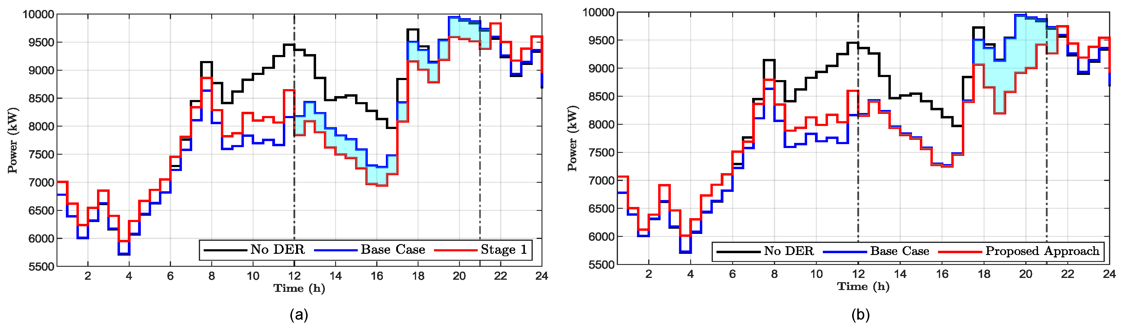
Case 1: No DER: a baseline scenario without any DER.

-

Case 2: Base Case: PV systems ($P{V}_1$ to $P{V}_4$) are optimally allocated within the DN, resulting in the base ADN.

-

Case 3: Proposed Two-Stage Scheduling Approach: a two-stage strategy is implemented, deploying the PV and BESS pairs ($P{V}_1$–$BES{S}_1$ for community 1 to $P{V}_4$–$BES{S}_4$ for community 4).

This section presents the optimal scheduling results for each BESS and evaluates the effectiveness of the proposed two-stage approach. Initially, the scheduling results are presented, demonstrating how minimizing the objective function reduces the maximum power fluctuations from the daily average net demand at the point of interconnection for each community, while also lowering the peak demand. Next, the performance of the approach under high cloud variability conditions is evaluated, with emphasis on utility demand, nodal voltage fluctuations at the community point of interconnections, and energy saved during peak shaving. This evaluation compares co-located PV systems operating with and without smart inverter (SI) control. When SI is enabled, the following control modes are considered: inductive constant power factor (CPF) at 0.91 lagging, IEEE 1547-2018 category B volt–VAr control, IEEE 1547-2018 category B volt–watt control, and a combined IEEE 1547-2018 category B volt–VAr/volt–watt control. Finally, the results from multi-core parallel processing are shown, demonstrating a reduction in QSTS simulation execution time.

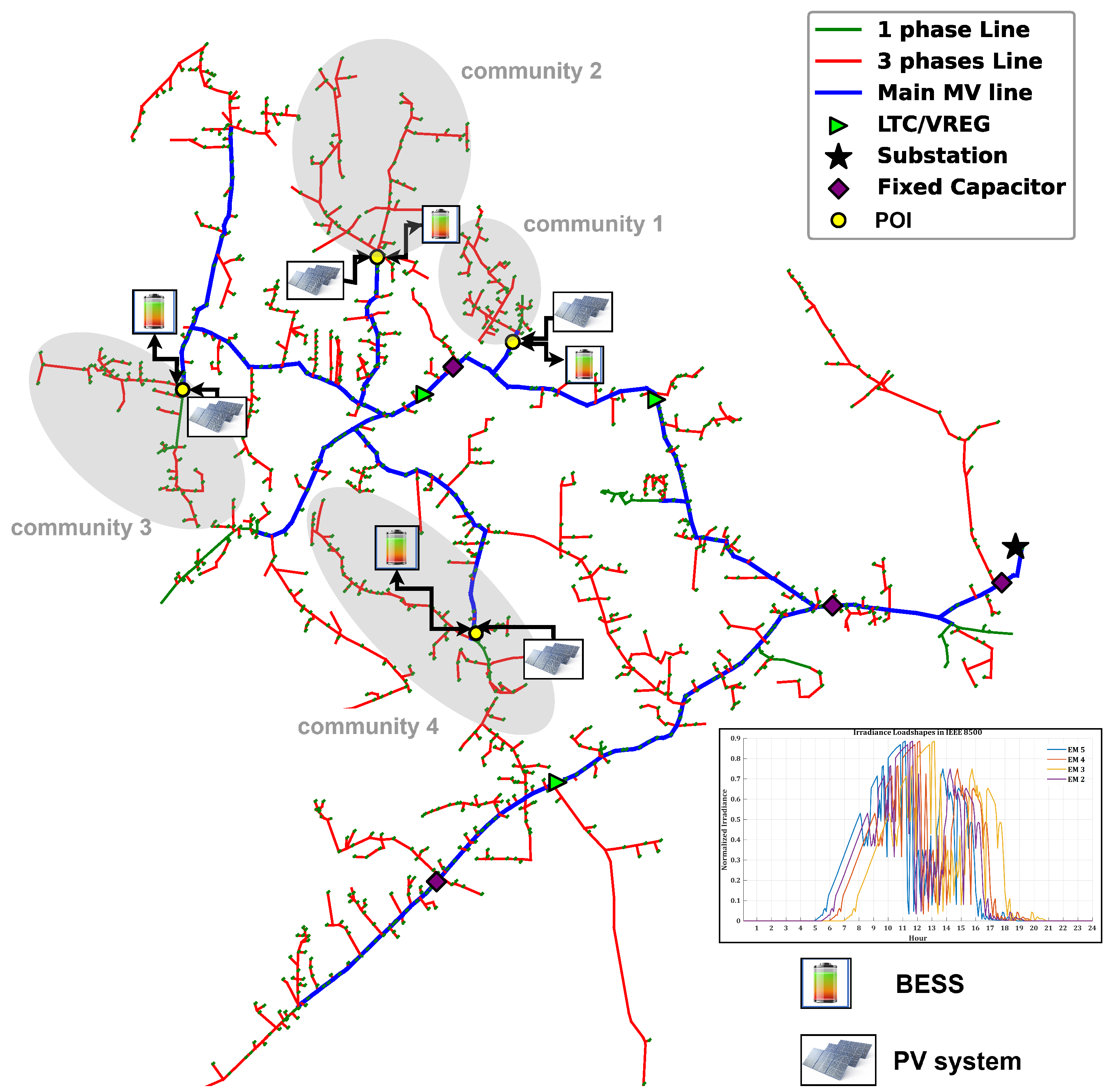
4.1. Specification of the Test DN

The proposed approach has been evaluated using the IEEE 8500-node test feeder [30], representing a large DN. The DN operates at a 7.2 kV base voltage with a total active load of 12.048 MW and a reactive load of 1.455 MVar. The feeder includes 12 single-phase voltage regulators, nine single-phase and one three-phase capacitor banks, over 2000 loads, about 1170 service transformers, and one substation transformer. Figure 6 shows the active distribution network test feeder with BESS integrated. The figure includes the nominal load demand and transition high cloud variability solar irradiance (SIR) profiles.

High-variability SIR profiles are independently assigned to each community to reflect geographical diversity and simulate the effects of localized cloud movement on the distribution network, as shown in the inset figure in Figure 6. This supports applicability to spatially proximate communities, each with distinct SIR. To determine each of the adjacent communities, energy meters are installed on the network to identify zones with large clusters of downstream customers. Power flow analysis is then performed to determine the active and reactive power consumption in these large clusters of high-demand zones. The nodes corresponding to these energy-metered zones with high demand are identified as POI for the co-located PV-BESS systems, as shown in Figure 6.

The ZIP load composition for the four communities is defined as Z = (0, 0), I = (0, 0), P = (1, 1). The DER-VET™ Tool [31] is used to determine the energy capacities and power ratings for each community’s BESS. By entering the community’s and utility load data, tariff rate structure, and BESS efficiency parameters, the tool performs techno-economic optimization to determine the optimal energy capacities and power ratings for peak shaving and load shifting. The resulting sizes reflect cost-effective configurations tailored to each community’s demand. This ensures that each BESS is properly sized to meet the specific energy needs of each community, preventing oversizing while still supporting peak demand shaving and energy shifting.

Table 2. Community components nominal rating.

Component	Community 1	Community 2	Community 3	Community 4
Demand Active Power [kW]	473	477	464	615
Demand Reactive Power [kVAr]	120.1	120.6	118.9	154
PV Power [kW]	500	500	500	500
BESS Power [kW]	321	330	321	425
BESS Energy [kWh]	1631	1646	1600	2120

summarizes the nominal ratings of each community’s components. The peak demand period is set from 12 pm to 9 pm, with an initial BESS SoC of 50% and charging and discharging efficiencies of 0.9. The inverter efficiency curve used is obtained from [32], while the maximum permissible line current has been set to 600 A.

The approach has been implemented using a fixed penalty coefficient, $c_{\mathit{p}}$ = ${10}^4$, determined through multiple trials and errors by testing multiple values to achieve a balance between constraint enforcement and optimization performance. The optimization has been carried out using N = 50 particles over a maximum of t = 50 iterations. The values for initial inertia weight w, damping ratio d, and the cognitive and social components are 1, 0.9, 2, and 2, respectively [27]. The day-ahead demand is obtained from [33], while the SIR data is sourced from [34].

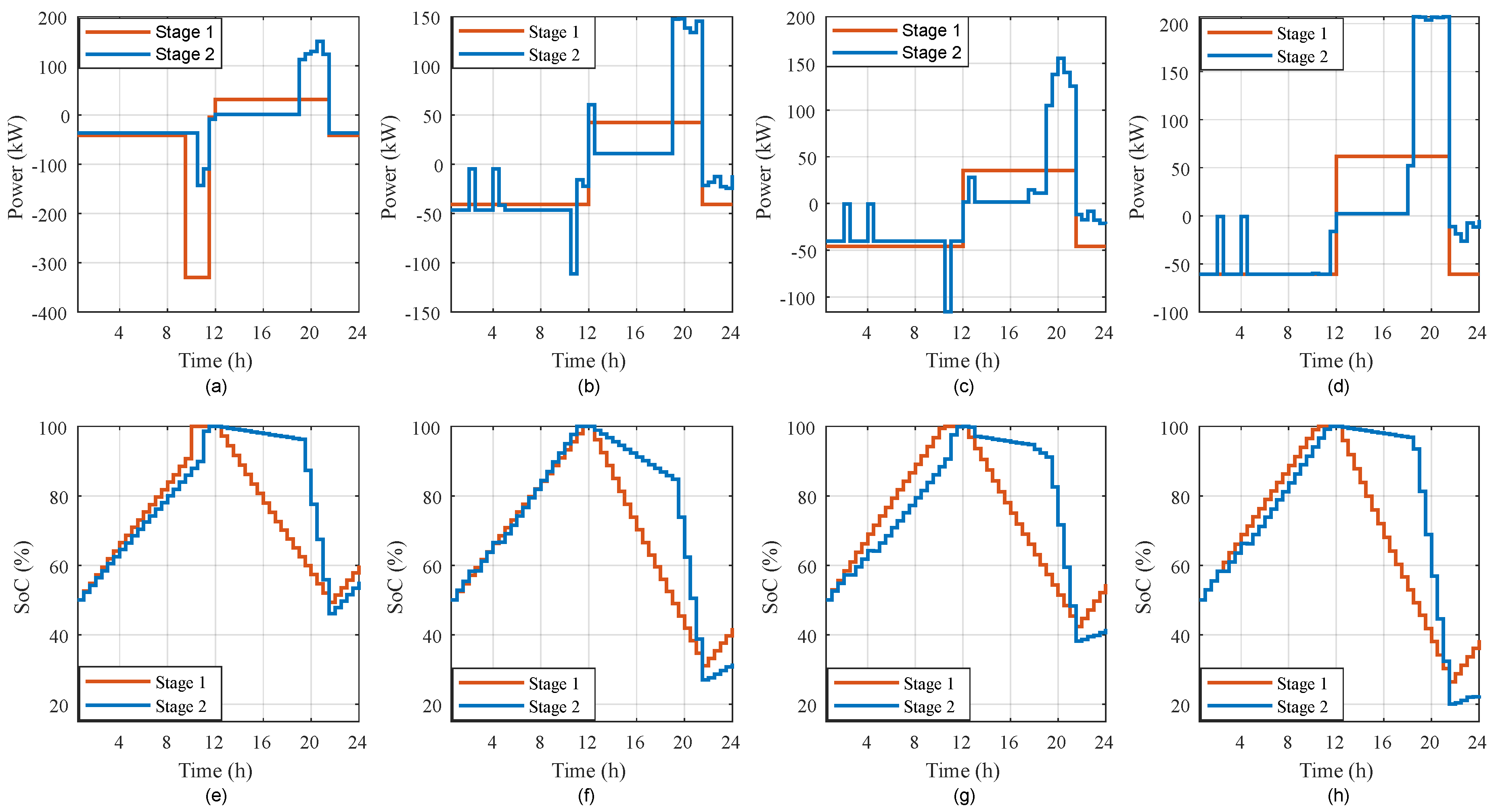
4.2. Scheduling Operation Results

Integrating BESSs with an active distribution network (ADN) mitigates the variations from intermittent PV output and lowers the peak demand, thereby addressing the voltage variations at the community point of interconnection (POI) that result from fluctuations in net demand. The proposed approach minimizes these power deviations by creating a new net demand profile with lower peak demand, leading to an optimal BESS charging and discharging schedule operation.

4.2.1. Results for Community PV Systems Without Smart Inverter Functions

When PV output power during variable SIR is injected into the ADN without reactive power support, i.e., smart inverter functionality is absent, it results in fluctuations at each community’s POI. The fluctuations lead to voltage deviations, especially during periods of variable SIR.

Each community’s BESS charges from PV and the grid during off-peak periods and discharges during peak periods. The percentage reduction in peak demand and standard deviation values is calculated as the ratio of the difference between the Stage 1 and Stage 2 values to the Stage 1 value, multiplied by 100, as shown below:

$$\% \mathrm{Reduction}=\left({\displaystyle \frac{\mathrm{Stage}{1}_{\mathrm{Value}}-\mathrm{Stage}{2}_{\mathrm{Value}}}{\mathrm{Stage}{1}_{\mathrm{Value}}}}\right)\times 100\%$$

(30)

The standard deviation used to evaluate demand variability, $\sigma$, is expressed as:

$$\sigma =\sqrt{{\displaystyle \frac{1}{M}}{\displaystyle \sum _{k=1}^M}{\left(D_k^{\mathrm{net}}-\overline{D^{\mathrm{net}}}\right)}^2}$$

(31)

where $D_k^{\mathrm{net}}$ is the net demand at the POI at time interval k, and $\overline{D^{\mathrm{net}}}$ is the mean net demand over M time intervals. Figure 7b illustrates that this approach decreases the peak demand of the ADN substation by 4.687%, lowering it from 9,932.3 kW in the base case to 9,466.81 kW in stage 2. This represents a notable improvement compared to the 2.067% reduction obtained in stage 1, as shown in Figure 7a. The BESS discharges power effectively, lowering the peak demand.

In stage 2, the BESS across all four communities decreased the ADN peak demand period energy by 1757.91 kWh, which represents a 0.125% increase compared to stage 1. However, most of this reduction occurs at the end of the SIR period, when PV output is absent, but peak demand remains high, as shown in Figure 7b.

Variations in cloud cover affect PV power output, resulting in power fluctuations within the ADN. During these fluctuations, each community’s BESS compensates for the reduced PV output by injecting additional power, as illustrated in Figure 8a–d. At the end of both the peak demand period and the day, each of the community’s BESS retains a SoC above the reserve level as seen in Figure 8e–h. This end-of-day SoC then serves as the initial SoC for the next day.

Given the stochastic nature of PSO in the stage 2 approach, a statistical analysis has been performed to assess the effectiveness of the proposed BESS scheduling approach. Ten independent PSO runs are executed using different random seeds to aid unbiased exploration of the solution space. Each independent PSO run corresponds to 48 sequential PSO runs (each sequence run occurs at the beginning of the interval/30 min), representative of the day. Figure 9a shows key statistical metrics — minimum, maximum, mean of the global best fitness—computed across the runs to evaluate convergence and solution quality for community 3. Figure 9b further illustrates its convergence behavior, which required the highest number of iterations to converge, 38. In contrast, all other communities converged within 25 iterations.

The average standard deviation of the PSO results quantifies how consistently the algorithm converges across runs, reflecting on the reliability of the heuristic scheduling approach despite PSO’s random nature. Community 3 shows the highest standard deviation at 6.769%, indicating a greater variability and a more complex or rugged optimization. This observation corresponds with Figure 9b, where community 3 required more iterations to reach convergence, while communities 1, 2, and 4 exhibit lower standard deviations of 4.158%, 5.034%, and 4.933%, respectively, suggesting smoother search spaces and faster convergence. Overall, these statistical metrics suggest that the proposed heuristic approach yields repeatable BESS schedules across different community zones, with community 3 posing a slightly more complex optimization challenge.

4.2.2. Results for Community PV Systems with Smart Inverter Functions

With smart inverter (SI) functionalities enabled, PV systems can provide reactive power support, reducing voltage fluctuations at each community’s POI. This functionality enhances the POI voltage reliability, especially during variable SIR conditions. Additionally, the optimal scheduling of BESSs further mitigates power deviations at the POI by absorbing excess PV energy and discharging during peak demand. Figure 10b illustrates that this approach decreases the ADN substation peak demand by 4.895%, lowering it from 9938.4 kW in the base case to 9451.9 kW in stage 2. This is an increase over the 3.494% reduction observed in stage 1, as shown in Figure 10a. The BESS in all four communities’ POI decreased peak demand energy by 2850.1 kWh in stage 2, an increase of 5.267% compared to stage 1. The BESS’s output increases towards the end of the peak demand period as PV power output reduces/ceases due to the absence of SIR similar to that shown in Figure 7b. The BESS SoC serves as the initial SoC for the next day.

Figure 11 illustrates the impact of smart inverter volt–VAr/volt–watt (VV/VW) control on nodal voltage and reactive power support across four ADN communities’ POIs over a 24 h period. Without SI control, the POI voltages show noticeable fluctuations, especially during SIR hours when PV output is intermittent, leading to increased voltage issues at each community’s POI. With the VV/VW control enabled, voltage profiles are significantly smoothed and maintained closer to the deadband region, effectively mitigating voltage rise. The corresponding reactive power plots show the amount of VAr absorbed by the smart inverter to mitigate this voltage rise. When the VAr output is zero, it indicates that the voltage remains within the deadband region and the VV/VW control is inactive. Outside this deadband range, the smart inverter dynamically absorbs VArs. These results confirm that the combined VV/VW control enhances voltage regulation and grid support at the monitored community POI.

4.3. Performance Evaluation of the Proposed Approach

The effectiveness of the approach has been evaluated by analyzing the comparison of utility peak demand, the demand standard deviation ($\sigma$), and total energy shaved for stage 1 and stage 2 for the communities’ PV system without and with smart inverter functionality. The percentage reductions presented in

Table 3. Evaluation of utility demand and energy shaved for system without smart inverter functions.

Scenario	Parameter	Without PSO (Stage 1)	With PSO (Stage 2)	% Reduction
Cloudy Irradiance	Peak Demand [kW]	9727	9466.81	2.675
	$\sigma ,\mu$ [kW]	1097.1 (8026.7)	1016.4 (7970.4)	7.356
	Energy Shaved [kWh]	1760.1	1757.9	0.125

and

Table 4. Evaluation of utility demand and energy shaved for system with combined VV/VW smart inverter function.

Scenario	Parameter	Without PSO (Stage 1)	With PSO (Stage 2)	% Reduction
Cloudy Irradiance	Peak Demand [kW]	9587.1	9451.96	1.409
	$\sigma ,\mu$ [kW]	1079.8 (7990.1)	989.5 (7988.7)	8.363
	Energy Shaved [kWh]	3010.64	2850.09	5.333

are computed using Equation (30). The utility demand results show a % decrease in standard deviation of up to 7.356%. This corresponds to a 2.675% drop in the ADN peak demand on a day with high cloud variability when the PV systems have no smart inverter functions enabled.

Moreover, when the PV systems have smart inverter functions enabled, there is a larger reduction in ($\sigma$) of up to 8.363% for a 1.409% reduction in ADN peak demand. The increased percentage reduction in the standard deviation of the net demand is attributed to the control provided by the smart inverter. The smart inverter control mitigates voltage fluctuations caused by variations in SIR, reducing the overall variability in net demand. Additionally, as shown in Table 4, there is a 1.409% reduction in peak demand for the smart inverter control function in stage 2. This reduction occurs because the smart inverter mitigates voltage variations at the monitored bus, thereby reducing the standard deviation of net demand. However, the smart inverter control results in more power being discharged from the BESS to compensate for the reduced PV output at the end of the peak demand horizon as seen in Figure 10b. Consequently, although the maximum demand level is lower, the overall energy shaving is greater.

To assess the impact of the SI functionality in providing voltage support during intermittent PV output power, which can occur due to variable cloud cover and changing load conditions, the voltage deviation index (VDI) performance metric is utilized. The VDI, which is the average absolute deviation of controlled voltages from the uncontrolled baseline (without SI functions), is expressed as:

$$\mathrm{VDI}={\displaystyle \frac{1}{M}}\sum _{k=1}^M\left|V_{\mathrm{controlled},k}-V_{\mathrm{uncontrolled},k}\right|$$

(32)

where $V_{\mathrm{controlled},i}$ and $V_{\mathrm{uncontrolled},k}$ are the POI nodal voltages at time interval k with and without SI functions, respectively, over M time intervals. The VDI assesses the steady-state voltage leveling provided by the smart inverter functionality. The approach aligns with goals for grid reliability and compliance with voltage standards, such as ANSI C84.1.

Table 5. Comparison of different SI functionalities for total energy and loss reduction in the DN.

Parameter	No DER	Without SI Functions	% Reduction
			VV	CPF	VW	VV/VW
Total Energy [MWh]	200.26	191.27	0.017 (0.032) MWh	0.037 (0.071)	0.065 (0.12)	0.114 (0.21)
Total DN Loss [MWh]	15.78	14.62	0.228 (0.033) MWh	0.397 (0.058)	0.096 (0.014)	0.484 (0.071)

presents the IEEE 8500 feeder-level parameters including daily energy consumed, and DN losses, for different smart inverter control modes. The percentage reduction in total energy consumed, as seen in Table 5, is due to the SI control functions’ focus on voltage support by managing the community’s POI voltage through reactive power injection. The SI control performs voltage support rather than reducing power demand at the DN substation. Table 5 also shows a decrease in total DN losses, attributed to reactive power injection bringing voltage closer to the deadband region. The constant power factor (CPF) mode, operating at 0.91 lagging PF, achieves a loss reduction of 0.397% (58.1 kWh). This is slightly less than the VV/VW mode, which attains a % loss reduction of 0.484% (70.8 kWh) as the volt–watt control (VW) curtails active power during overvoltage conditions.

Table 6. VDI % reduction in community POI nodal voltages for different SI control modes in comparison to without SI functions.

POI Phases	VV				CPF				VW				VV/VW
	Community				Community				Community				Community
	1	2	3	4	1	2	3	4	1	2	3	4	1	2	3	4
node a	14.05	12.54	12.61	9.66	20.89	14.42	14.81	14.73	0.56	0.87	0.45	0.48	17.96	15.99	12.66	11.32
node b	4.41	6.28	1.92	7.46	10.29	10.06	13.77	10.94	0.10	0.28	0.12	0.18	35.45	32.17	28.81	31.45
node c	4.01	1.78	0.41	1.93	15.54	9.05	11.22	17.00	0.95	14.81	14.45	12.96	15.96	37.63	34.29	26.71

validates the effectiveness of different SI functions in regulating voltage profiles at community POIs. Table 6 shows that the VV/VW mode achieves the largest VDI % reduction up to 37.632% at community 2’s POI. This enhanced regulation is attributed to the combined effect of reactive power injection and active power curtailment by the SI control, although some variability remains. Additionally, the CPF mode achieves a maximum VDI % reduction of 20.891% at community 1’s POI, reflecting its limited dynamic response due to fixed power factor operation. The VW mode achieves the lowest % reduction in VDI among the evaluated SI control modes.

Notably, node a across all community POIs exhibits the greatest VDI % reduction, indicating the unbalanced nature of the community loads in the DN.

4.4. Computational Complexity

Multiple factors influence the execution time for BESS scheduling, including circuit size and topology, power system computations, device specifications, and parameters related to the optimization approach. The optimized BESS scheduling’s execution time for each time interval is compared to the sequential processing case to highlight the benefits of parallel processing. The proposed approach achieved a 69.482% reduction in computation time when compared to sequential processing. Figure 12 illustrates the execution time of QSTS simulations for both the sequential and parallel processing CPU implementation schemes.

Thread allocation plays a critical role in determining the solution time for each actor, as execution is distributed across threads based on system workload and hardware capabilities. Figure 13 illustrate the computational time for each CPU core across different time intervals of the simulation. Results show that the time for solution varies between individual CPU cores. The solution times are influenced by thread allocation and the proposed algorithm’s ability to reach optimal BESS scheduling for each time interval taken by each core.

5. Conclusions

This paper validates a proposed two-stage approach for optimizing BESS scheduling for peak shaving operation in an ADN, with a primary focus on reducing execution time. In the first stage, a rule-based decision tree determines the initial BESS operation setpoints for heuristic optimization. In the second stage, a PSO algorithm optimizes the BESS charge and discharge schedule for peak shaving and valley filling. The approach has been evaluated across four adjacent BESS communities under high cloud variability conditions in the IEEE 8500-node DN. The effect of different smart inverter functions, namely CPF, VV control, VW control, and combined VV/VW control, is analyzed to assess their voltage support capabilities. Results indicate that the proposed scheduling approach reduces peak demand by up to 4.895%, and also decreases the overall demand standard deviation by up to 8.363% in smart inverter-enabled scenarios. Additionally, the nodal voltage deviation index (VDI) is reduced by 37.632% when operating in VV/VW mode. The implementation of parallel processing on multiple CPU cores improved computational efficiency by 69.482% compared to sequential processing, underscoring the scalability of the approach for large distribution networks. Such a two–stage scheduling approach with parallel processing has potential to enhance BESS utilization in ADN, thereby helping to reduce peak demand and mitigate power deviations in the distribution network.

References

1. Amako, E.A.; Arzani, A.; Mahajan, S.M. Optimal Sizing of PV Systems in a Utility Distribution Feeder Using OpenDSS. In Proceedings of the 56th North American Power Symposium (NAPS), Boston, MA, USA, 13–15 October 2024; pp. 1–6. [Google Scholar] [CrossRef]
2. U.S. Energy Information Administration. Solar, Battery Storage to Lead New U.S. Generating Capacity Additions in 2025; Today in Energy; U.S. Energy Information Administration: Washington, DC, USA, 2025. Available online: https://www.eia.gov/todayinenergy/detail.php?id=64586 (accessed on 31 May 2025).
3. Ruiz-Cortés, M.; González-Romera, E.; Amaral-Lopes, R.; Romero-Cadaval, E.; Martins, J.; Milanés-Montero, M.I.; Barrero-Gonzalez, F. Optimal Charge/Discharge Scheduling of Batteries in Microgrids of Prosumers. IEEE Trans. Energy Convers. 2019, 34, 468–477. [Google Scholar] [CrossRef]
4. Sun, Z.; Eskandari, M.; Zheng, C.; Li, M. Handling Computation Hardness and Time Complexity Issue of Battery Energy Storage Scheduling in Microgrids by Deep Reinforcement Learning. Energies 2023, 16, 90. [Google Scholar] [CrossRef]
5. Zhang, X.; Son, Y.; Choi, S. Optimal Scheduling of Battery Energy Storage Systems and Demand Response for Distribution Systems with High Penetration of Renewable Energy Sources. Energies 2022, 15, 2212. [Google Scholar] [CrossRef]
6. Abbasi, A.; Alves, F.; Ribeiro, R.A.; Sobral, J.L.; Rodrigues, R. Optimizing Virtual Power Plants with Parallel Simulated Annealing on High-Performance Computing. Smart Cities 2025, 8, 47. [Google Scholar] [CrossRef]
7. Bose, B.K. Power Electronics in Renewable Energy Systems and Smart Grid: Technology and Applications; John Wiley & Sons: Hoboken, NJ, USA, 2019. [Google Scholar]
8. Rana, M.M.; Romlie, M.F.; Abdullah, M.F.; Uddin, M.; Sarkar, M.R. A Novel Peak Load Shaving Algorithm for Isolated Microgrid Using Hybrid PV-BESS System. Energy 2021, 234, 121157. [Google Scholar] [CrossRef]
9. Cienfuegos, C.; Rodrigo, P.M.; Cienfuegos, I.; Diaz-Ponce, A. Comparative Analysis of Battery Energy Storage Systems’ Operation Strategies for Peak Shaving in Industries with or without Installed Photovoltaic Capacity. Renew. Energy Focus 2024, 49, 100574. [Google Scholar] [CrossRef]
10. Li, F.; Li, X.; Zhang, B.; Li, Z.; Lu, M. Multiobjective Optimization Configuration of a Prosumer’s Energy Storage System Based on an Improved Fast Nondominated Sorting Genetic Algorithm. IEEE Access 2021, 9, 27015–27025. [Google Scholar] [CrossRef]
11. Karandeh, R.; Lawanson, T.; Cecchi, V. A Two-Stage Algorithm for Optimal Scheduling of Battery Energy Storage Systems for Peak-Shaving. In Proceedings of the 2019 North American Power Symposium (NAPS), Wichita, KS, USA, 13–15 October 2019; pp. 1–6. [Google Scholar] [CrossRef]
12. Arzani, A.; Venayagamoorthy, G.K. Computational Approach to Enhance Performance of Photovoltaic System Inverters Interfaced to Utility Grids. IET Renew. Power Gener. 2018, 12, 112–124. [Google Scholar] [CrossRef]
13. Dimas, C.; Ramos, G.; Caro, L.; Luna, A.C. Parallel Computing and Multicore Platform to Assess Electric Vehicle Hosting Capacity. IEEE Trans. Ind. Appl. 2020, 56, 4709–4717. [Google Scholar] [CrossRef]
14. Saldarini, A.; Longo, M.; Brenna, M.; Zaninelli, D. Battery Electric Storage Systems: Advances, Challenges, and Market Trends. Energies 2023, 16, 7566. [Google Scholar] [CrossRef]
15. Moghaddam, I.N.; Chowdhury, B.H.; Mohajeryami, S. Predictive Operation and Optimal Sizing of Battery Energy Storage With High Wind Energy Penetration. IEEE Trans. Ind. Electron. 2018, 65, 6686–6695. [Google Scholar] [CrossRef]
16. Qing, K.; Huang, Q.; Chen, S.; Hu, W.; Wang, J. Optimized Operating Strategy for a Distribution Network Containing BESS and Renewable Energy. In Proceedings of the IEEE PES Innovative Smart Grid Technologies Asia (ISGT Asia), Kuala Lumpur, Malaysia, 22–25 April 2019; pp. 1593–1597. [Google Scholar] [CrossRef]
17. Bowen, T.; Chernyakhovskiy, I.; Denholm, P. Grid-Scale Battery Storage: Frequently Asked Questions; U.S. Department of Energy: Golden, CO, USA, 2019. Available online: https://www.nrel.gov/docs/fy19osti/74426.pdf (accessed on 24 February 2024).
18. Denholm, P.L.; Margolis, R.M. The Potential for Energy Storage to Provide Peaking Capacity in California Under Increased Penetration of Solar Photovoltaics; National Renewable Energy Lab. (NREL): Golden, CO, USA, 2018. [CrossRef]
19. IEEE Std 1547-2018; IEEE Standard for Interconnection and Interoperability of Distributed Energy Resources with Associated Electric Power Systems Interfaces. IEEE: Nwe York, NY, USA, 2018. [CrossRef]
20. Yoshizawa, S.; Yanagiya, Y.; Ishii, H.; Hayashi, Y.; Matsuura, T.; Hamada, H.; Mori, K. Voltage-Sensitivity-Based Volt-VAR-Watt Settings of Smart Inverters for Mitigating Voltage Rise in Distribution Systems. IEEE Open Access J. Power Energy 2021, 8, 584–595. [Google Scholar] [CrossRef]
21. Mirafzal, B.; Adib, A. On Grid-Interactive Smart Inverters: Features and Advancements. IEEE Access 2020, 8, 160526–160536. [Google Scholar] [CrossRef]
22. Amako, E.A.; Arzani, A.; Mahajan, S.M. BESS Scheduling for Two Communities of an Active Distribution Network. In Proceedings of the 2025 IEEE Texas Power and Energy Conference (TPEC), Houston, TX, USA, 20–22 February 2025; pp. 1–6. [Google Scholar] [CrossRef]
23. OpenDSS Documentation. Power Delivered to the Circuit. Available online: https://opendss.epri.com/Powerdeliveredtothecircuit.html (accessed on 24 February 2024).
24. ANSI C84.1-2020; Electric Power Systems and Equipment–Voltage Ratings (60 Hz). ANSI: Washington, DC, USA, 2020.
25. Parsopoulos, K.E.; Vrahatis, M.N. On the computation of all global minimizers through particle swarm optimization. IEEE Trans. Evol. Comput. 2004, 8, 211–224. [Google Scholar] [CrossRef]
26. Xue, B.; Zhang, M.; Browne, W.N. Particle Swarm Optimization for Feature Selection in Classification: A Multi-Objective Approach. IEEE Trans. Cybern. 2013, 43, 1656–1671. [Google Scholar] [CrossRef] [PubMed]
27. Shi, Y.; Eberhart, R. A modified particle swarm optimizer. In Proceedings of the 1998 IEEE International Conference on Evolutionary Computation, IEEE World Congress on Computational Intelligence, Anchorage, AK, USA, 4–9 May 1998; pp. 69–73. [Google Scholar] [CrossRef]
28. Mashayekhi, M.; Harati, M.; Estekanchi, H.E. Development of an alternative PSO-based algorithm for simulation of endurance time excitation functions. Eng. Rep. 2019, 1, e12048. [Google Scholar] [CrossRef]
29. Montenegro, D.; Dugan, R.C.; Reno, M.J. Open Source Tools for High Performance Quasi-Static-Time-Series Simulation Using Parallel Processing. In Proceedings of the 2017 IEEE 44th Photovoltaic Specialist Conference (PVSC), Washington, DC, USA, 25–30 June 2017; pp. 3055–3060. [Google Scholar] [CrossRef]
30. Arritt, R.F.; Dugan, R.C. The IEEE 8500-Node Test Feeder. In Proceedings of the IEEE PES T&D 2010, New Orleans, LA, USA, 19–22 April 2010; pp. 1–6. [Google Scholar] [CrossRef]
31. EPRI. Distributed Energy Resource Value Estimation Tool (DER-VET™ v1.2); Program 94; EPRI: Palo Alto, CA, USA, 2022. [Google Scholar]
32. EPRI. Modeling High-Penetration PV for Distribution Interconnection Studies: Smart Inverter Function Modeling in OpenDSS, Rev. 3; 3002011305; EPRI: Palo Alto, CA, USA, 2017. [Google Scholar]
33. Karanki, S.B.; Xu, D. Optimal Capacity and Placement of Battery Energy Storage Systems for Integrating Renewable Energy Sources in Distribution System. In Proceedings of the 2016 National Power Systems Conference (NPSC), Mumbai, India, 13–15 December 2016; pp. 1–6. [Google Scholar] [CrossRef]
34. National Renewable Energy Laboratory (NREL). NSRDB: National Solar Radiation Database. Available online: https://nsrdb.nrel.gov/data-viewer (accessed on 24 February 2025).
Figure 1. Volt–VAr control curve.
Electricity 06 00036 g001
Figure 2. Volt–watt control curve.
Electricity 06 00036 g002
Figure 3. Sequential vs. parallel processing concept for multi-community BESS scheduling.
Electricity 06 00036 g003
Figure 4. MATLAB–OpenDSS parallel processing subroutine.
Electricity 06 00036 g004
Figure 5. Proposed BESS scheduling algorithm flowchart.
Electricity 06 00036 g005
Figure 6. IEEE 8500-bus ADN with integrated BESS (insert: transition high cloud variability SIR profiles).
Electricity 06 00036 g006
Figure 7. DN substation demand for scenario without smart inverter during (a) conventional BESS scheduling approach (stage 1), (b) proposed BESS scheduling approach (stage 2).
Electricity 06 00036 g007
Figure 8. Each community BESS performance during stage 1 and stage 2. (a) P BESS 1 , (b) P BESS 2 , (c) P BESS 3 , (d) P BESS 4 , (e) SoC for BESS 1, (f) SoC for BESS 2, (g) SoC for BESS 3, (h) SoC for BESS 4.
Electricity 06 00036 g008
Figure 9. PSO solution randomness over 10 independent PSO runs, for community 3 BESS scheduling, (a) minimum, maximum, and mean global best fitness values ( P BESS ), (b) fitness function convergence evaluation.
Electricity 06 00036 g009
Figure 10. DN substation demand for scenario with smart inverter: (a) conventional BESS scheduling approach (stage 1), (b) proposed BESS scheduling approach (stage 2).
Electricity 06 00036 g010
Figure 11. Average nodal POI voltage and SI VAr output for communities 1 to 4 with VV/VW control and without control.
Electricity 06 00036 g011
Figure 12. QSTS simulation execution time for the CPU implementation scheme with (a) sequential processing, (b) parallel processing.
Electricity 06 00036 g012
Figure 13. CPU cores computation time for each simulation time-step (parallel processing).
Electricity 06 00036 g013