Noise Effects on Detection and Localization of Faults for Unified Power Flow Controller-Compensated Transmission Lines Using Traveling Waves

Abstract

This paper presents a comprehensive analysis of the effects of noise on the detection and localization of faults in transmission lines compensated with a unified power flow controller using traveling wave-based methods. This study focuses on the impact of harmonic and transient noises, which are inherent to power generation, transmission, and UPFC operation. A novel algorithm is proposed combining the Discrete Wavelet Transform and Clarke Transform to detect and localize faults under various noise conditions. The algorithm is tested on a simulated transmission line model in MATLAB/Simulink (Version R2022b) with noise levels of 20 dB, 30 dB, and 40 dB and transient frequencies of 1 kHz, 5 kHz, and 10 kHz. The results demonstrate that the algorithm achieves an average fault localization error of 0.523% under harmonic noise and 0.777% under transient noise, with fault detection rates of 96.3% and 90.75%, respectively. This study highlights the robustness of the traveling wave method in noisy environments and provides insights into the challenges posed by UPFC-compensated lines.

1. Introduction

Electric power transmission lines are among the most critical infrastructures, as they are responsible for transporting electricity from generation sites to cities, communities, or any location where electronic and electrical devices are needed [1]. However, they are also one of the components of the electrical system most susceptible to failures due to their extensive length, manufacturing conditions, environmental threats, and other internal and external factors [2]. Faults in transmission lines can cause blackouts, network imbalances, and the inability to meet the desired electrical demand. Moreover, noise and disturbances in transmission lines can further compromise reliability, complicating their operation and stability [3].

The protection of these lines is focused on quickly isolating faults to maintain system stability, and transmission companies are responsible for detecting and preventing future failures. With the advancement of smart grids and the increasing complexity of electrical systems, advanced monitoring has become crucial, particularly for transmission lines that are difficult to access [4]. In recent years, systems have been developed to detect rapid dynamic events, and studies have focused on improving the reliability and security of the system [4].

In recent times, flexible alternating current transmission systems (FACTS)-compensated transmission lines are a cost-effective option for transporting large volumes of wind energy over long distances [5]. Among FACTS devices, the unified power flow controller (UPFC) has recently stood out for its ability to manage active and reactive power flow [5] independently. Furthermore, the various UPFC operating practices also cause rapid changes in the line impedance. Consequently, conventionally used distance relay-based transmission line protection schemes encounter limitations in ensuring fast and reliable protection, in addition to various problems that could arise with UPFC, including noise generated on transmission lines, generators, and the UPFC device itself [5].

Wavelet transform-based methods are inherently susceptible to noise [1]. Furthermore, there is no specific procedure for specifying the appropriate mother wavelet type and the optimal number of decomposition levels, and they must be determined by trial and error [5]. There are several studies on how noise affects the detection, location, and classification of faults in transmission lines, with or without FACTS compensators [6]. The proposed method in [7] for phasor estimation in fault current analysis within series-compensated transmission lines proves effective, especially under challenging off-nominal frequency conditions. Comprehensive simulations validate its robustness, showing a mean absolute error below 1% in amplitude and 1° in phase estimation. Additionally, the method maintains accuracy even with signal-to-noise ratios as low as 30 dB, making it a reliable tool for fault location applications in power systems.

The protection scheme in [5] operates in two main stages. First, it uses spectral energy ratios from the grid-side current, extracted via variational mode decomposition at 4 kHz, to distinguish internal faults from external and transients. A Wiener filter denoises the signal in both stages to improve accuracy. Research [4] presents an ITD-based fault detection scheme designed to address the unique challenges of photovoltaic power plants in distance relay applications. The scheme effectively handles noise, with simulations demonstrating accuracy at noise levels up to 20 dB, alongside other conditions like high fault resistance and varying irradiance.

The research in [8] introduces a method for fault classification and localization in transmission lines using phasor measurement unit data and a Weighted Extreme Learning Machine (WELM) optimized by the Grey Wolf Optimization (GWO) algorithm. By leveraging a wavelet-based feature extraction method, the GWO-WELM model achieves high accuracy, 99.83% in classification and 95.48% in localization. Additionally, it demonstrates robustness under noise, maintaining classification and localization accuracies of 91.5% and 88.1%, respectively, at a 10 dB signal-to-noise ratio.

In [1], the research focuses on monitoring transmission lines using traveling wave theory, addressing the challenge posed by noise and the variable propagation characteristics of the lines. The method utilizes complex continuous wavelet transform to analyze time-series data from simulations on the IEEE 39-bus system. It is particularly adept at handling noise, as demonstrated with a Gaussian noise level of 60 dB SNR. The approach effectively identifies incident and reflected waves. However, it is observed that noise does increase the error in the results, although these are still within the range of error values handled by other state-of-the-art works.

Papers related to detection, location, and classification in transmission lines have shown that they are functional considering scenarios with noise. Besides, it is necessary to analyze the different magnitudes of noise considering the noise related to the electric generation element; the transmission lines; and, if they exist, the FACTS devices in the network. The last is the one whose noise analysis has been studied the least when the approach is carried out using the traveling wave.

Therefore, it is essential to analyze how disturbances generated by devices such as UPFCs impact the propagation of traveling waves used in fault localization. The sensitivity of these waves to high-frequency distortions, combined with the limited attention this phenomenon has received in the literature, highlights a significant gap. This need motivated the development of the proposed algorithm, aimed at improving the reliability and accuracy of fault detection and localization in compensated transmission systems under real-world noise scenarios.

This research performs an analysis for the detection, classification, and location of faults in transmission lines compensated with a UPFC device considering different noise scenarios in the network, in different sections, and through traveling waves, considering that due to its nature of analysis, they are sensitive to noise, especially high-frequency noise.

This work’s contribution lies in analyzing the noises inherent to the generation, transmission, and compensation device by means of the traveling wave in noisy scenarios considering a UPFC compensation device.

The following sections analyze the different types of noise found in generators and transmission lines as well as those caused by FACTS devices; following this, the analysis of the applied computational techniques, the description of the network, and the experiments performed are presented. Then, the following section continues with the development, followed by Section 6, and finally ends with Section 7.

Regarding the use of technological tools during the writing of this manuscript, an artificial intelligence tool (ChatGPT, OpenAI, version 2025) was occasionally used for the sole purpose of optimizing grammatical aspects of the English language, such as the choice of conjunctions and correcting the use of verb tenses. No artificial intelligence was used for the generation of academic content, data analysis, figure creation, methodological design, or interpretation of results. All scientific, conceptual, and experimental work was carried out entirely and in its original form by the authors.

2. Noise Problems in Protection Schemes on Compensated Transmission Lines

Noise in electrical systems refers to any unwanted electrical signals that interfere with the proper functioning of devices, such as protection schemes. One prevalent type of noise is electromagnetic interference (EMI), which arises from the coupling of electromagnetic fields generated by various sources [9]. Common sources of EMI include nearby equipment like motors, generators, or high-voltage switching as well as external disturbances such as lightning strikes or solar flares. The mechanism of EMI involves inducing unwanted voltages or currents in the measurement or control circuits, potentially corrupting signals used by protection relays [9].

Another significant type of noise is harmonic distortion, which consists of higher-frequency components of the fundamental power system frequency (50/60 Hz) [10]. Non-linear loads or compensation devices often generate these harmonics. On compensated transmission lines, series capacitors and shunt devices can introduce significant harmonic content, distorting current and voltage waveforms and leading to errors in measurement and protection operation [10].

Switching transients also contribute to noise [11], characterized by high-frequency, short-duration surges caused by switching operations such as those involving capacitor banks or circuit breakers. These transients can resemble fault conditions, potentially triggering false trips in protection systems. Similarly, signal aliasing occurs when high-frequency noise is sampled at an insufficient rate, causing it to appear as low-frequency components in the sampled signal [11]. This phenomenon can mislead digital relays, especially those using digital signal processing (DSP). Environmental noise, including electrical noise from weather-related disturbances [12] like lightning and noise from mechanical vibrations in transformers or generators, can also couple into protection circuitry, particularly in systems with inadequate shielding or grounding.

The presence of noise in electrical systems significantly affects the accurate detection and discrimination of faults in transmission systems [1]. One major impact is incorrect fault detection, where noise signals can mimic fault conditions, causing protection systems to isolate healthy parts of the grid or mask actual fault signals, delaying or preventing the detection of genuine faults. Noise can also lead to the misoperation of relays, which process current and voltage signals to calculate fault parameters.

Electrically compensated transmission lines introduce unique challenges due to the interaction of compensation devices with noise [13]. The dynamic response of compensation devices adds further complexity. These devices respond dynamically to load or fault condition changes, with rapid switching generating high-frequency transients that may overlap with fault signals, confusing protection schemes. Moreover, the frequency-dependent behavior of compensated lines complicates protection schemes, as the impedance of these lines varies with frequency. Noise signals at different frequencies interact with compensation devices in distinct ways, altering their characteristics and challenging the reliance of protection schemes on consistent system parameters.

3. Techniques and Methods Used

Digital signal processing techniques and transformations based on mathematical operations are the basis for the analysis and development of different processes as well as the detection and location of faults in compensated transmission lines. In this section, the techniques and operations used in the development of this work are briefly described with the purpose of a simple reconstruction of the experiment.

3.1. Discrete Wavelet Transform

Wavelet transform is a signal processing technique that evolved from Fourier Transform and hort-Time Fourier Transform [14]. Unlike its predecessors, wavelet transform allows for the adjustment of both time and frequency resolution. It includes two main types: continuous wavelet transform (CWT) and Discrete Wavelet Transform (DWT) [14].

In the case of DWT, signals are analyzed by scaling the frequency and shifting the position across discrete time intervals, as represented in (1).

$$DWT(m,n)={\displaystyle \frac{1}{\sqrt{2^m}}}{\sum }_{k}f(k)\phi \left[{\displaystyle \frac{n-k{2}^m}{2^m}}\right],$$

(1)

In this equation, $m$, $n$, and $k$ are integers that represent key parameters of the transformation. The symbol $\phi$ refers to the mother wavelet, which serves as the foundational function for wavelet transform. The variable n denotes the number of data points in the signal, m represents the scaling factor that adjusts the frequency resolution, and $k$ indicates the shifting factor used to localize the wavelet in time.

DWT separates the original signal into two frequency bands: high-frequency and low-frequency components. Each decomposition step reduces the frequency range by half compared to the previous step. This multiresolution analysis allows the DWT filter to break the signal down into specific frequency ranges, facilitating signal analysis and processing [14].

3.2. Clarke Transform

Clarke transform is a method used to convert three-phase voltage into three components: $\alpha$, $\beta$, and $\gamma$ [15]. The $\alpha$ and $\beta$ components represent projections on the real and imaginary axes, while the γ component corresponds to the zero-sequence component. After a short circuit fault on the transmission line, the $\alpha$, $\beta$, and $\gamma$ components exhibit noticeable changes. The fluctuation of the $\gamma$ component reflects the degree of voltage imbalance, enabling the real-time and accurate detection of transmission line faults [15].

The components of the transformed voltage ($v_{\alpha }$, $v_{\beta }$, $v_{\gamma }$) are calculated as follows:

$$\left[\begin{array}{c}{v}_{\alpha }\\ v_{\beta }\\ v_{\gamma }\end{array}\right]=\mathit{C}\left[\begin{array}{c}{v}_a\\ v_b\\ v_c\end{array}\right]=\left[\begin{array}{ccc}{\displaystyle \frac{2}{3}}& -{\displaystyle \frac{1}{3}}& -{\displaystyle \frac{1}{3}}\\ 0& \sqrt{{\displaystyle \frac{1}{3}}}& -\sqrt{{\displaystyle \frac{1}{3}}}\\ {\displaystyle \frac{1}{3}}& {\displaystyle \frac{1}{3}}& {\displaystyle \frac{1}{3}}\end{array}\right]\left[\begin{array}{c}{v}_a\\ v_b\\ v_c\end{array}\right],$$

(2)

where $\mathit{C}$ is the Clarke transform matrix, and $v_a$, $v_b$, and $v_c$ are the three-phase voltages of the system.

3.3. The Traveling Wave

The traveling wave method leverages the reflections of electromagnetic waves generated by faults or discontinuities along a transmission line [16]. When a fault occurs, traveling waves propagate along the line, reflecting at each point of discontinuity, including the fault location and the line’s endpoints. This method analyzes these reflections to identify the correct peaks required for fault distance calculation [16].

Traditionally, two key time instants, $t_1$ and $t_{end}$, corresponding to specific peaks, are used to determine the fault distance. These time instants are analyzed using the well-established Equations (3) and (4).

$$d_1={\displaystyle \frac{(t_1-t_0)v_0}{2}},$$

(3)

$$d_{end}=L_{end}{\displaystyle \frac{(t_{end}-t_0)v_0}{2}},$$

(4)

In these equations, $d_1$ represents the distance from the initial point of the transmission line to the fault, while $d_{end}$ represents the distance from the end of the transmission line to the fault. The variable $t_0$ corresponds to the time when the wave is initiated, often marking the moment the fault occurs. $t_1$ and $t_{end}$ denote the arrival times of the traveling waves at the detection points near the line’s start and end, respectively. The propagation speed of the traveling wave, $v_0$, depends on the transmission line’s physical properties. Lastly, $L_{end}$ represents the total length of the transmission line.

Calculating these distances allows the fault’s precise location along the transmission line to be determined, enabling timely and accurate fault detection and mitigation [16].

During a transmission line fault, pulses are generated at the point of incidence, which propagate in opposite directions toward the ends of the line. These disturbances produce high-frequency traveling waves that are captured by the relays installed at the ends [17]. During the event, the relays also record the interaction between the harmonic frequencies generated by the UPFC and the traveling waves. The voltage at any point “x” on the line is described by (5).

$$V_x=V_{-}{e}^{-\gamma x}+V_{+}{e}^{+\gamma x},$$

(5)

where $\gamma$ is the propagation coefficient, $V_{-}{e}^{-\gamma x}$ represents the incident wave, and $V_{+}{e}^{+\gamma x}$ is the reflected wave from the remote end.

4. Network Description and Tests Performed

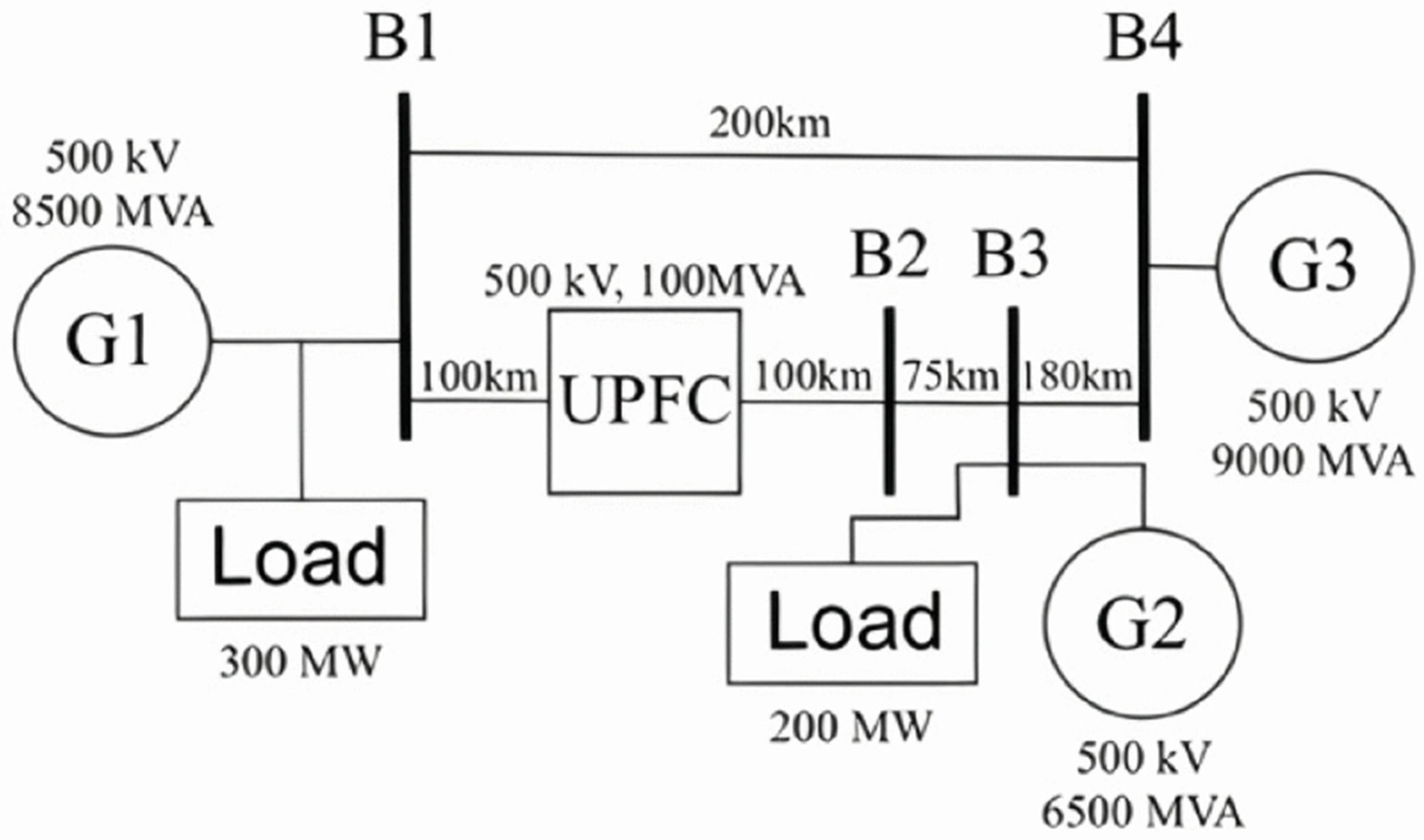
The network used to simulate the different fault scenarios is described in [17], a previous work produced by our research group. This study addresses the need to determine whether, under noisy conditions, the traveling wave concept for fault detection and location maintains similar levels of accuracy.

The UPFC is positioned between the local bus (B1) and the remote bus (B2). Figure 1 illustrates the properties of the three generators, G1, G2, and G3. The system includes two loads, one at B1 and another at B3, operating at a fundamental frequency of 60 Hz and a voltage level of 500 kV.

The system model was developed in MATLAB/SIMULINK. A simulation duration of one second was chosen, with 80,000 samples collected, resulting in a sampling rate of 80 kHz. The voltage measurements obtained at the local bus B1 from this model was utilized to analyze the data using the algorithm proposed in this study.

The noise incorporated into the simulations consisted of two types: harmonic noise and transient noise. In this context, a detailed analysis of harmonic and transient noise in a transmission line compensated with a UPFC was conducted. The UPFC, as a device for active and reactive power control, can modify the current and voltage waveforms on the line, influencing the generation and propagation of these types of noise.

For harmonic noise, the 3rd, 5th, and 7th harmonics were considered because they are the most common in industrial and commercial networks, as established in [18]. These harmonics are typically generated by nonlinear loads and have a considerable impact on voltage and current waveforms. Regarding the SNR level (20, 30, and 40 dB), these values were chosen to represent high, medium, and low signal-to-noise ratio conditions, such as those found in real-world environments with electromagnetic interference or transients. This selection is consistent with practices described in previous studies and with the recommendations of [19], which establishes requirements for evaluating the performance of acquisition systems under different noise levels.

The amount of noise in a transmission line compensated with a UPFC can be primarily adjusted through the regulation of active and reactive power flow, voltage, waveform control, switching frequency, filter implementation, and the system’s dynamic response optimization. These parameters influence both harmonic distortion and transients, enabling control over power quality in the network.

The analysis of the signals was performed using the voltage signals measured at the local end, and the added noise signals of the two types that we studied, which were harmonic noise and transient noise caused by switching events, were added at the output of the UPFC device.

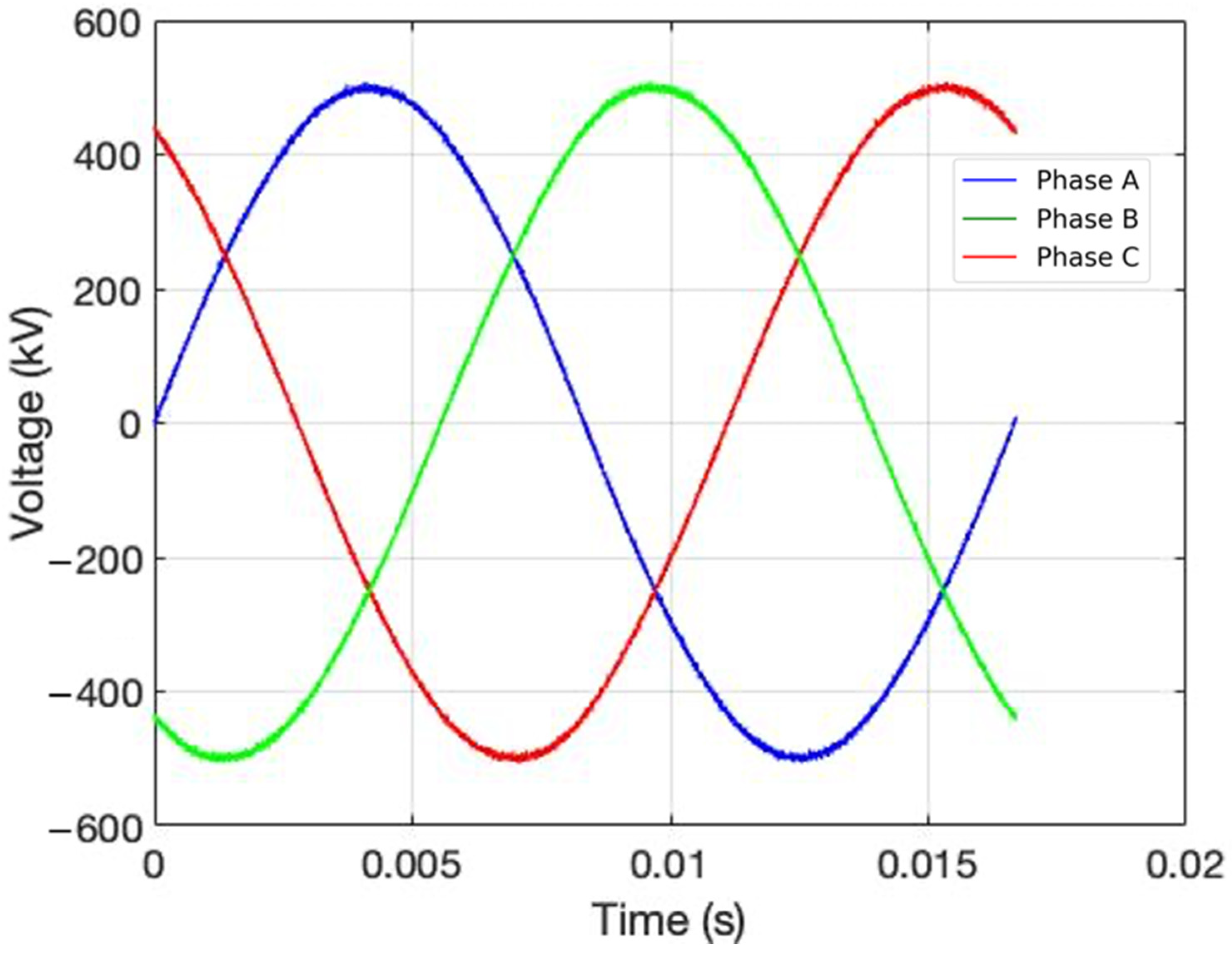
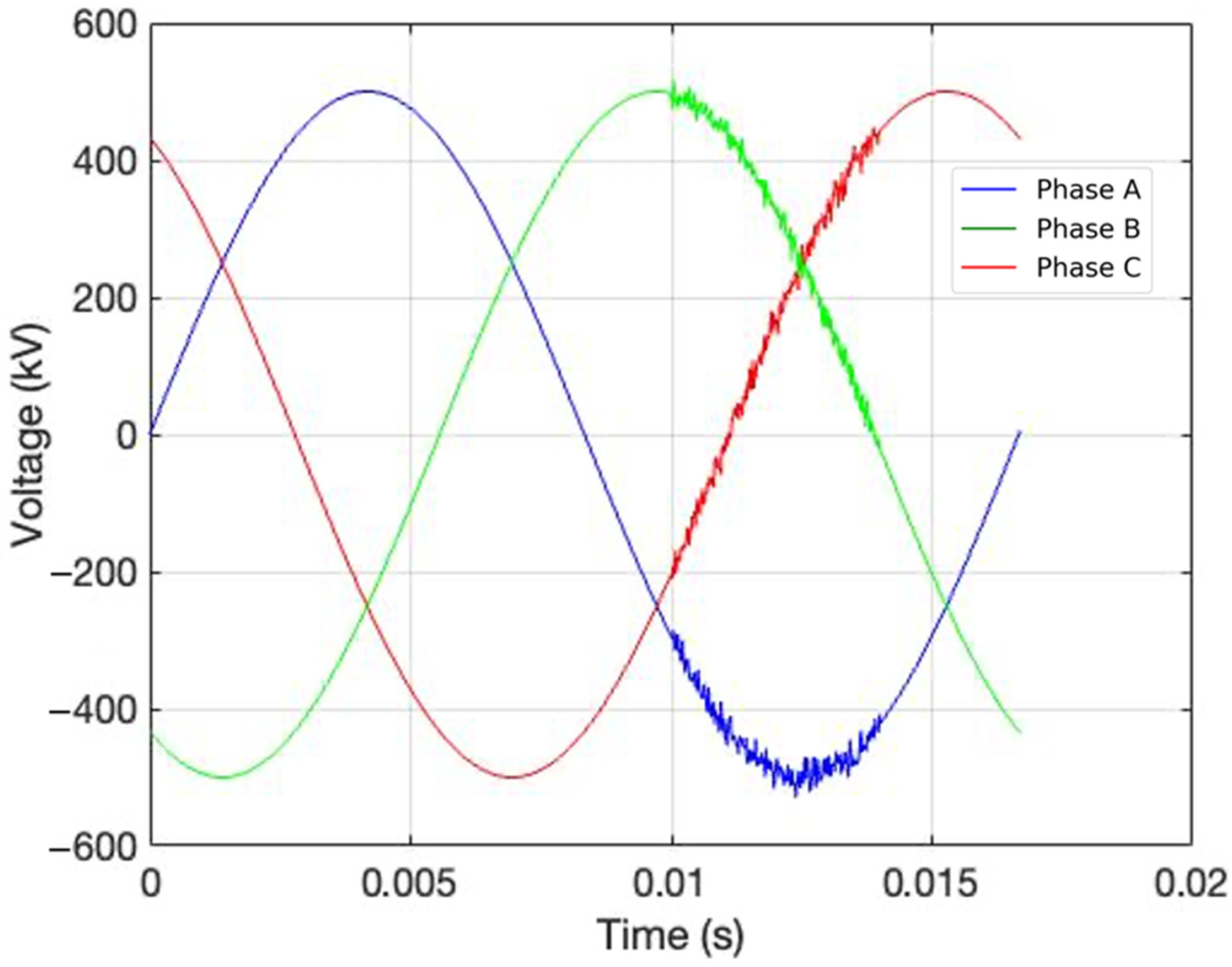
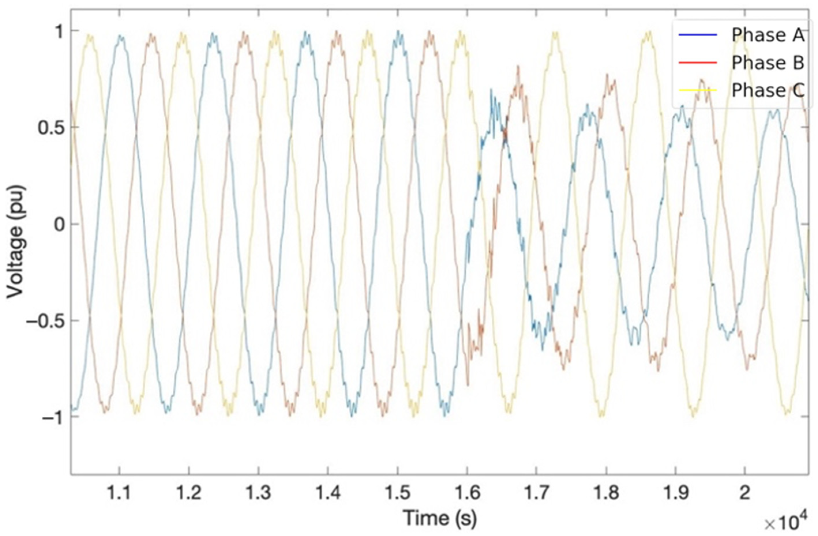
In Figure 2, the signal measured at the local end with harmonic noise is observed, while in Figure 3, the signal with noise caused by transients is shown.

Due to the nature of the traveling wave-based algorithm, which is sensitive to frequency changes, it is of great relevance to determine whether comparable results can be obtained with those from previous studies. This study assesses whether this technique can be effectively applied under noisy conditions. Considering the state of the art, the noise analysis was conducted with noise levels of 20 dB, 30 dB, and 40 dB relative to the voltage signals. Consequently, the noise was incorporated into the voltage signals.

From Equation (6), the necessary noise voltage for the corresponding analysis was derived, and the results are summarized in

Table 1. Results for added noise voltage.

Noise (dB)	Noise Magnitude (kV)	Percentage Relative to Original Signal
20	50	10%
30	15.81	3.16%
40	1.58	1%

.

$$dB=20log\left({\displaystyle \frac{V_{noise}}{V_{signal}}}\right),$$

(6)

where dB is the noise level in decibels, and $V_{signal}$ is the voltage of 500 kV observed at the local end due to generation. Table 1 summarizes the process of the values used.

The transient noise generated by UPFC switching operations exhibits frequencies ranging from 1 kHz to 10 kHz. For the analysis, noise frequencies of 1 kHz, 5 kHz, and 10 kHz were selected as representative values.

Fault locations were set at distances of 70 km, 80 km, 90 km, 110 km, 120 km, and 130 km from the local bus. At each location, 11 distinct fault types were simulated, with a fault inception angle of 36° and fault resistance level of 25 $\mathsf{\Omega }$. The fault types included AB, AC, BC, AG, BG, CG, ABG, ACG, BCG, ABC, and ABCG. Since the values are expressed in per unit, all voltage outputs from the model fall within the range of −1 to 1.

Therefore, considering all fault types and the six proposed distances, a total of 594 simulations were analyzed for the case of harmonic noise. This analysis accounted for the three different suggested noise levels and three possible scenarios: the presence of the third harmonic; the presence of the third and fifth harmonics; and the presence of the third, fifth, and seventh harmonics. Similarly, for the case of transient noise, 594 simulations were analyzed to incorporate the three proposed decibel levels and the three proposed frequencies.

5. Development of Noise Analysis

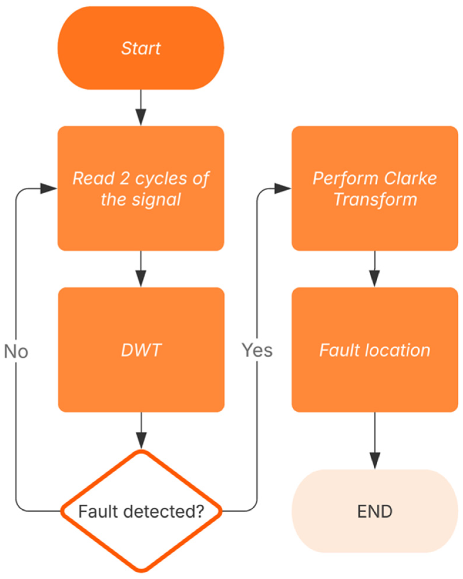
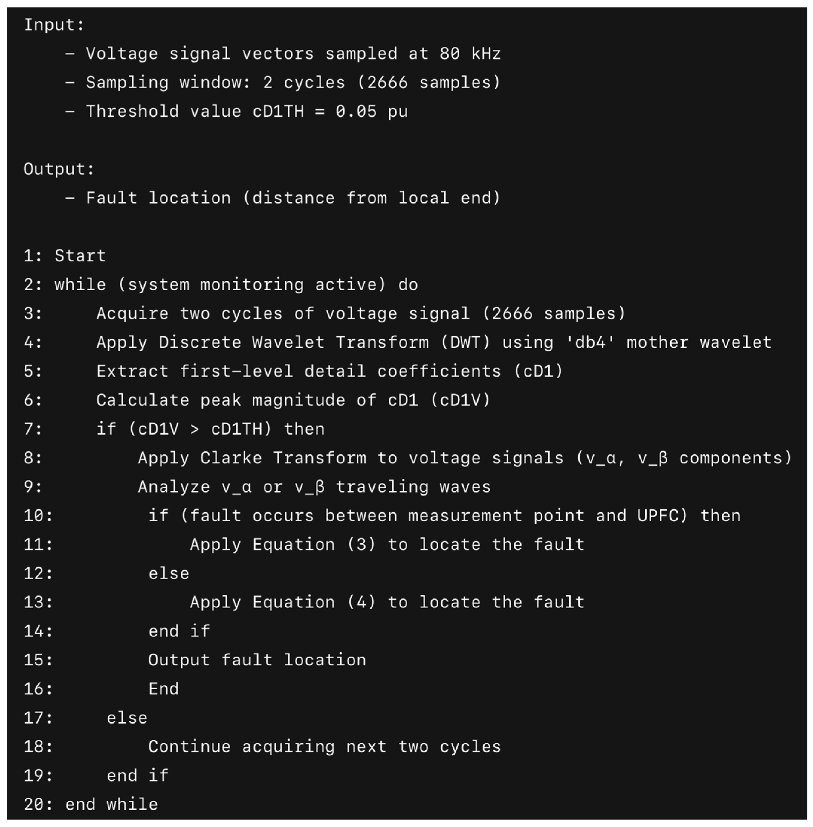
In this section, we present the algorithm used in our study, which employs traveling waves for fault detection and localization. Figure 4 illustrates the methodology along with a discussion of key points. The primary objective is to analyze the influence of noise on the accuracy and reliability of fault detection and localization.

At the start of the algorithm, two cycles of the 60 Hz sinusoidal signals are captured. Given a sampling frequency of 80 kHz, 2666 samples are used to represent each instance of two signal cycles.

Following this, the DWT is applied to the voltage signal vectors. Using the Daubechies 4 mother wavelet, the first-level detail coefficients (cD₁) are extracted. This process enables the identification of frequency-related signal changes, providing critical insights into their behavior.

For fault detection, the magnitude of the peak in the wavelet detail coefficients (cD_1V) is calculated. A fault is detected if cD_1V exceeds a predefined threshold (cD_1TH). The threshold cD_1TH is typically set to 5% of the peak voltage value. This algorithm uses a value of 0.05, as the voltage range is expressed in per-unit (pu) values. This approach ensures the detection of faults along the line. If a fault is detected, the algorithm proceeds to the next step. Otherwise, it returns to the signal cycle acquisition step to obtain the next two cycles and analyze whether a fault has occurred. This process repeats iteratively.

Once the two cycles where the fault was detected are identified, the Clarke transform is applied to the signals. This transformation allows the extraction of components in which the fault-induced traveling waves propagate and reflect. By analyzing these components, the exact moment of the fault can be observed and localized.

By analyzing the $v_{\alpha }$ or $v_{\beta }$ signals, either (3) or (4) is applied. Equation (3) is used if the fault occurs between the measurement point and the UPFC (i.e., in the first half of the line from the local end). Equation (4) is applied if the fault occurs beyond the UPFC, toward the remote end of the line. In the latter case, the traveling waves continue propagating toward the remote end and are subsequently reflected back. The process for determining which equation to apply, based on the fault location, the components involved, and the number of measurement devices used, is further detailed in [16,17].

For a better understanding of the process, the pseudocode of the algorithm shown in Figure 4 is observed in Figure 5. To apply the DWT, the “pywt.dwt()” function was applied, and for the CT, it was implemented by creating matrix (2) with the numpy library.

6. Results

In this section, we present the outcomes of the simulations conducted to evaluate the performance of the proposed algorithm for fault detection and localization. The results include fault detection errors and fault precision under various conditions. Additionally, the impact of noise on the algorithm’s reliability is analyzed. These findings provide critical insights into the effectiveness of the methodology and its robustness in real-world scenarios.

Out of 594 simulations conducted under noisy conditions with harmonics, the algorithm successfully detected faults in 572 cases. The only instances where faults were not accurately detected occurred under 20 dB noise levels in the presence of the third, fifth, and seventh harmonics (16 failures). This resulted in an error rate of 3.7% for fault detection under harmonic noise conditions. The error rate for simulations involving transient noise was higher at 9.25%, with 539 out of 594 simulations correctly identifying the fault. This increase in error is attributed to the frequency-domain characteristics of the traveling waves during fault events.

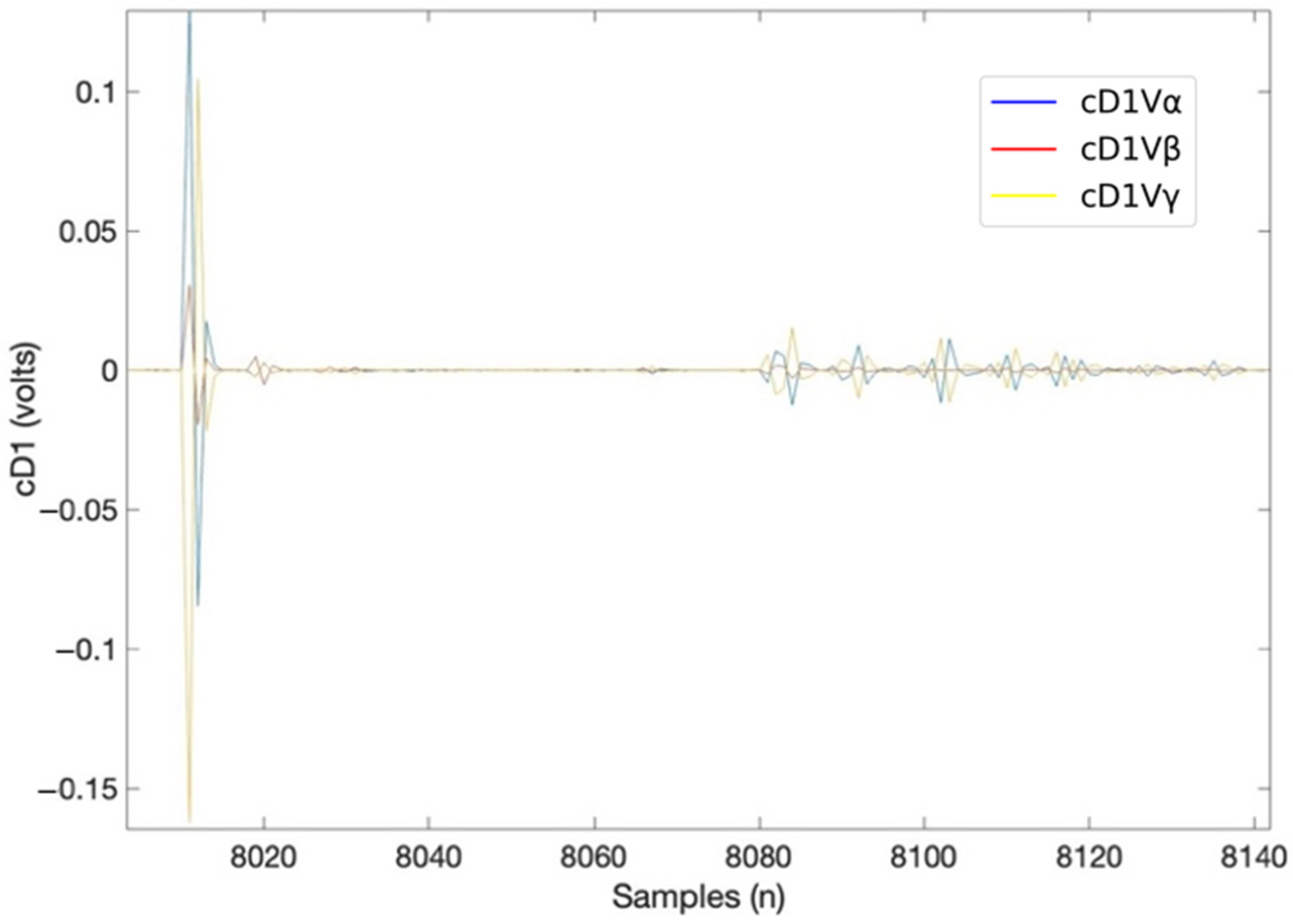
Figure 6 illustrates the signal with 30 dB harmonic noise at the moment of the fault. In contrast, Figure 7 shows the first-level detail coefficients (DWT) extracted simultaneously, providing insight into the fault detection process.

Due to the complexity of displaying all data simultaneously, two representative tables are provided.

Table 2. Results with harmonic noise.

Fault Type	dB	Fault Applied (km)						Error %
		70	80	90	110	120	130
AB	20	70.42	81.54	90.80	109.3	120.5	127.9	0.501
	30	72.27	81.54	90.80	111.2	120.5	129.7	0.545
	40	70.42	79.68	90.80	109.3	118.6	129.7	0.324
AC	20	72.27	79.68	88.95	111.2	122.3	131.6	0.725
	30	70.42	81.54	88.95	111.2	120.5	129.7	0.411
	40	70.42	79.68	90.80	111.2	122.3	127.9	0.597
BC	20	68.57	79.68	88.95	109.3	118.6	129.7	0.429
	30	70.42	79.68	88.95	111.2	122.3	127.9	0.618
	40	70.42	79.68	88.95	109.3	120.5	129.7	0.265
AB	20	70.42	81.54	90.80	109.3	120.5	127.9	0.501
	30	70.42	77.83	88.95	109.3	120.5	131.6	0.527
	40	70.42	77.83	88.95	111.2	122.3	127.9	0.772
AG	20	70.42	79.68	90.80	109.3	122.3	129.7	0.399
	30	68.57	79.68	88.95	109.3	122.3	129.7	0.504
	40	70.42	79.68	90.80	109.3	120.5	131.6	0.352
BG	20	72.27	79.68	88.95	111.2	120.5	131.6	0.571
	30	70.42	81.54	88.95	109.3	118.6	131.6	0.554
	40	70.42	79.68	90.80	109.3	122.3	131.6	0.507
CG	20	68.57	79.68	88.95	111.2	118.6	129.7	0.472
	30	70.42	81.54	88.95	109.3	122.3	127.9	0.676
	40	72.27	79.68	88.95	109.3	120.5	129.7	0.420
ABG	20	70.42	81.54	90.80	109.3	120.5	127.9	0.501
	30	68.57	79.68	90.80	111.2	122.3	131.6	0.635
	40	70.42	79.68	88.95	109.3	118.6	127.9	0.499
ACG	20	68.57	77.83	88.95	109.3	120.5	129.7	0.504
	30	70.42	77.83	88.95	109.3	120.5	127.9	0.574
	40	70.42	79.68	90.80	111.2	122.3	129.7	0.443
BCG	20	72.27	81.54	88.95	109.3	120.5	131.6	0.629
	30	70.42	77.83	88.95	109.3	118.6	127.9	0.653
	40	70.42	79.68	90.80	109.3	122.3	127.9	0.554
ABC	20	72.27	79.68	88.95	111.2	120.5	131.6	0.571
	30	68.57	81.54	90.80	109.3	118.6	129.7	0.510
	40	70.42	81.54	88.95	109.3	122.3	129.7	0.522
ABCG	20	70.42	81.54	90.80	109.3	120.5	127.9	0.501
	30	72.27	81.54	90.80	111.2	120.5	129.7	0.545
	40	70.42	79.68	90.80	109.3	118.6	129.7	0.324

presents the localization results for the 11 fault types, evaluated under three different noise levels (in decibels), with the presence of the third, fifth, and seventh harmonics. Similarly,

Table 3. Noisy results due to transients.

Fault Type	dB	Fault Applied (km)						Error %
		70	80	90	110	120	130
AB	20	72.27	77.83	88.95	109.3	122.3	127.9	0.883
	30	72.27	77.83	88.95	107.5	118.6	131.6	0.915
	40	70.42	79.68	87.10	109.3	120.5	127.9	0.574
AC	20	68.57	81.54	87.10	111.2	118.6	129.7	0.729
	30	72.27	81.54	90.80	109.3	122.3	131.6	0.763
	40	70.42	79.68	90.80	109.3	120.5	127.9	0.399
BC	20	72.27	81.54	90.80	107.5	122.3	127.9	0.964
	30	68.57	77.83	90.80	107.5	118.6	127.9	0.872
	40	72.27	79.68	90.80	111.2	122.3	129.7	0.597
AB	20	68.57	77.83	90.80	109.3	122.3	127.9	0.793
	30	70.42	81.54	88.95	107.5	120.5	127.9	0.676
	40	68.57	77.83	87.10	107.5	118.6	129.7	0.892
AG	20	68.57	81.54	87.10	111.2	122.3	127.9	0.959
	30	70.42	81.54	90.80	111.2	122.3	131.6	0.652
	40	68.57	77.83	87.10	107.5	122.3	131.6	1.075
BG	20	72.27	77.83	90.80	111.2	118.6	129.7	0.676
	30	68.57	77.83	87.10	111.2	122.3	127.9	1.011
	40	70.42	81.54	90.80	111.2	120.5	131.6	0.498
CG	20	72.27	81.54	88.95	109.3	118.6	131.6	0.708
	30	70.42	77.83	87.10	111.2	122.3	131.6	0.880
	40	68.57	81.54	90.80	107.5	122.3	131.6	0.848
ABG	20	68.57	81.54	88.95	111.2	118.6	131.6	0.682
	30	68.57	79.68	87.10	111.2	122.3	131.6	0.810
	40	68.57	77.83	87.10	111.2	120.5	131.6	0.810
ACG	20	68.57	77.83	87.10	111.2	118.6	129.7	0.781
	30	68.57	81.54	90.80	111.2	122.3	131.6	0.737
	40	72.27	79.68	87.10	111.2	120.5	129.7	0.618
BCG	20	72.27	81.54	90.80	111.2	118.6	127.9	0.778
	30	72.27	77.83	87.10	109.3	122.3	127.9	1.038
	40	68.57	79.68	88.95	109.3	118.6	127.9	0.583
ABC	20	68.57	77.83	87.10	111.2	122.3	129.7	0.857
	30	72.27	81.54	90.80	111.2	122.3	131.6	0.807
	40	68.57	77.83	90.80	111.2	122.3	131.6	0.789
ABCG	20	72.27	77.83	88.95	109.3	122.3	127.9	0.883
	30	72.27	77.83	88.95	107.5	118.6	131.6	0.915
	40	70.42	79.68	87.10	109.3	120.5	127.9	0.574

provides equivalent localization results for the same 11 fault types and noise levels but with transient frequencies of 10 kHz. These tables highlight the algorithm’s performance under varying conditions, offering a comprehensive overview of its accuracy and robustness.

The transmission line length (TLL) is incorporated as a critical parameter in the analysis to assess the error and rigorously enable a more accurate comparison. Accordingly, the error is computed using the following mathematical expression (7).

$$error={\displaystyle \frac{\left|calculated value-actual value\right|}{TLL}}$$

(7)

It is important to highlight that the present study conducts the analysis under noisy conditions, whereas the referenced work in [17] performs the same evaluation in a noise-free environment. This distinction allows for a direct comparison of results and an assessment of the impact of noise on the accuracy of the proposed method.

For example, if the first pulse is received in sample 10 and the second pulse is received in sample 48, or due to its sampling frequency (80 kHz), at window times 0.125 ms and 0.6 ms, respectively, applying Formula (3), the location of the fault is 70.42 km. Because we know the location at which the fault was generated is 70 km, applying Formula (7), we can determine that the error is 0.21%.

Table 2 demonstrates that the fault location results align with the traveling wave’s intrinsic behavior at the specified sampling frequency. The average error in fault location was 0.523%, where harmonic noise had a greater impact on fault detection than on localization accuracy. A similar effect was observed (Table 3) with transient noise, although it contributed more significantly to error percentages than harmonic noise. The average fault location error increased to 0.777% since transient noise, which exhibits similarities with the disturbances generated by the fault, led to a higher number of detection errors.

Although the results obtained confirm a general trend of decreasing localization error with increasing SNR, slight fluctuations in localization accuracy were observed. These variations are attributable to the inherent sensitivity of the traveling-wave method to high-frequency distortions, which, due to the non-stationary and frequency-dependent nature of the harmonic noise considered, affect system behavior in a nonlinear manner. These effects explain the occasional discrepancies recorded in some test scenarios, without compromising the overall validity of the observed trend or the robustness of the proposed method for fault detection and localization.

7. Conclusions

The analysis of noise effects on fault detection and localization in UPFC-compensated transmission lines using traveling waves has yielded significant insights. The proposed algorithm, which combines the DWT and Clarke transform, has proven effective in detecting and localizing faults under various noise conditions, including harmonic and transient noise. The results indicate that the algorithm maintains a high level of accuracy, with an average fault localization error of 0.523% under harmonic noise and 0.777% under transient noise. The fault detection rates were 96.3% and 90.75%, respectively, demonstrating the algorithm’s robustness in noisy environments.

The study reveals that harmonic noise has a greater impact on fault detection than on localization accuracy, while transient noise, due to its similarity to fault-induced disturbances, contributes more significantly to localization errors. The algorithm’s performance is consistent across different fault types, distances, and noise levels, making it a reliable tool for real-world applications. However, the presence of noise, particularly at lower signal-to-noise ratios, can lead to missed detections, especially in scenarios with multiple harmonics or high-frequency transients.

The findings also highlight the importance of considering noise sources from generators, transmission lines, and UPFC devices when designing protection schemes. The dynamic behavior of UPFCs, combined with the frequency-dependent characteristics of transmission lines, adds complexity to fault detection and localization. Future work should focus on further optimizing the algorithm to reduce sensitivity to noise and improve detection rates under extreme conditions. Additionally, integrating advanced filtering techniques and machine learning models could enhance the algorithm’s performance in real-time applications.

Since the presented results were obtained through simulations performed in Matlab/Simulink with a sampling rate of 80 kHz, it was considered essential to analyze their compliance with current IEEE technical standards. Specifically, the proposed fault detection and localization method is based on the traveling wave technique, based on [20], which guides fault localization in transmission lines. Furthermore, [21], related to FACTS devices and in particular to the UPFC, which is integrated into the simulated system, was taken into account. The high sampling rate employed allows for accurate representation of wavefronts, even under noisy conditions, which reinforces the validity of the simulated results within the context of practical applications and the technical margins defined by said standards.

The proposed method offers a promising solution for fault detection and localization in UPFC-compensated transmission lines, even in the presence of significant noise. The results align with the intrinsic behavior of traveling waves and provide a foundation for further research in this area, particularly in the context of modern power systems with increasing levels of renewable energy integration and FACTS devices.