Forecasting Average Daily and Peak Electrical Load Based on Average Monthly Electricity Consumption Data

Abstract

This article is devoted to the determination of the average daily electric load and the average electric load during the hours of maximum load, taking into account the generalized coefficient A_i, using data on electricity consumption for apartment buildings and individual residential buildings in Chelyabinsk and the cities of Dushanbe and Khorog in the Republic of Tajikistan. The results of modeling the average daily electric load, taking into account the developed generalized coefficient A_i, showed that the specific power values for apartments in apartment buildings and in individual residential buildings in the city of Chelyabinsk and the cities of Dushanbe and Khorog of the Republic of Tajikistan were overestimated, taking into account the applicability in the Republic of Tajikistan of the same standard values of specific electric loads (SELs) for apartments in apartment buildings (ABs) as in the Russian Federation. According to the results of modeling using data on the average monthly electricity consumption for 226 apartments in ABs and for individual residential buildings in Chelyabinsk, and according to the proposed approach, the average daily electric load on days during the month varied in the range of 2–3.5 kW/sq and below, while that for the cities of Dushanbe and Khorog of the Republic of Tajikistan varied in the range of 2–5 kW/sq and below, which did not exceed the SEL given by RB 256.1325800.2016. However, because of the lack of other energy sources (gas supply and hot water supply) in the conditions of the Republic of Tajikistan, on the basis of the obtained maximum load time factor and the generalized coefficient ${\mathrm{A}}_{\mathrm{i}\left(\mathrm{E}\right)}$, the obtained values of actual capacity exceeded the maximum during peak hours by 1.2–2.5 times the SEL given by RB 256.1325800.2016. To increase the durability and serviceability of power supplies and enhance the effectiveness of forecasting, the authors propose an approach based on the clustering of meteorological conditions, where each cluster has its own regression model. The decrease in mean absolute error due to clustering was 0.52 MW (57%). The use of meteorological conditions allowed the forecast error to be reduced by 0.22 MW (27%). High accuracy in electrical consumption forecasting leads to increased quality of power system management in general, including under such key indicators as reliability and serviceability.

1. Introduction

In the context of the transition to decarbonization, one of the most effective ways to provide electricity to consumers is the use of autonomous power supply systems [1,2,3]. Earlier, in [4,5,6,7,8,9,10,11,12], clarifications to the classification of autonomous power supply systems (APSs) were proposed. In particular, APSs with a capacity of up to 10 kW and over 10 to 100 kW were introduced, and justifications for these proposals were given.

For an APS with a capacity of up to 10 kW, it is recommended to use a power supply scheme with two-wire lines with wires insulated from the ground, since in such systems, single-phase electric receivers are used as consumers of electric energy [13,14,15,16,17,18]. In APS with a capacity of up to 100 kW, the presence of three-phase consumers is possible.

The scope of application of APSs with a capacity of 10 to 100 kW is currently extensive. They can be used in the following cases:

• In the absence of a centralized power supply;
• If it is not possible to connect to the centralized power supply system;
• For remote objects;
• For dachas, small houses, trade stalls;
• For remote warehouses, cabins, houses at recreation centers;
• For power, remote video surveillance and communication;
• For power supply of fire and security alarms;
• For weather stations;
• For auto coffee shops;
• For autotourism, etc.

Basically, such systems are used to provide electricity to private households and farms such as apiaries, cheese dairies, and greenhouses [19,20,21]. As power sources, photovoltaic (solar) batteries and wind turbines receive the most popular demand. However, it is economically inexpedient to provide for the presence of an energy service in the structure of such enterprises.

When switching to autonomous power supply systems, a number of issues should be solved, one of which is uninterrupted supply [22,23,24,25]. Problems with these systems that remain to this day include low efficiency and the inconsistency of the primary source (wind, water, etc.).

However, in the course of operation of these systems, a problem arises related to the establishment of the causes of constant disruption to reliability and energy efficiency associated with frequent untimely output of equipment from sources of autonomous power supply systems. The problem of the correspondence of the actual electric load to the specific power with apartment buildings [1,2,3,4,5,6,7] and individual residential buildings [8] has become significant in recent years.

The term “actual specific power of the electric load” is understood as the ratio of the average monthly power consumption (obtained from the data of electricity meters installed at consumers of apartment buildings) or the average monthly power consumption at peak hours (based on the results of measurements at morning and evening peaks at the entrance to apartments) to the number of days and hours in the month or at peak hours.

Meanwhile, the term “specific power of the electric load” is understood as the ratio of the design capacity to the number of apartments, taking into account the presence or absence of gas supply and centralized hot and cold water supply in the apartments.

The inconsistencies of autonomous power supply systems, noted in [1,2,3,4,5,6,7,9], lead already at the design stage of the power supply systems of apartment buildings and private housing construction to the creation of prerequisites for disruption of the operating mode in 6–10/0.4 kV distribution electric networks. Numerous studies conducted by various groups of scientists in the Republic of Tatarstan, a number of cities of the Russian Federation (Moscow, Moscow Region) [26], and the Chelyabinsk Region [26,27,28] have shown an excess of specific power over actual specific power. However, there are practically no similar studies for individual housing construction.

As is known, in order to establish the correspondence between the actual and specific power, the most accurate approach is to take measurements (30 min, hourly), which allows you to determine the actual power of the apartment in the AB at the moment. However, due to the increase in actual power associated with a number of factors [26,28], the application of the results obtained on the basis of electric load measurements for forecasting electricity consumption is not always correct, complex and costly. The costs are due, first of all, to the need to carry out repeated measurements with a frequency of 2–3 years in order to adjust the specific capacity.

The most appropriate way to determine the actual power is to use the data of average monthly electricity consumption. It should be noted that the application of the results of previous electricity consumption to predict the electric load without identifying the factors that create the expected electrical load of apartments leads to large errors and, as a result, requires adjustment based on measurements.

Therefore, in order to minimize the cost and time, as well as to exclude the constant adjustment (with a period every 2–3 years) of the specific power in the current realities, it is possible to predict the expected actual electric power of apartments in apartment buildings and private housing construction based on the data of the average monthly electricity consumption, while taking into account the factors that create these loads.

To solve the problem of forecasting the power consumption of the electric power system, such well-known metrics as MAPE, MAE and RMSE are widely used.

The examination of neural network training for short-term electrical consumption forecasting is carried out [29]. The authors correlate the actual and predicted curve with the daily mean absolute percentage error (MAPE). The best daily MAPE value is 1.58%, and the worst is 25.38%; this error is due to two holidays. Further research is needed to develop a program that considers changes in electrical consumption due to holidays.

The authors of the article [26] developed a real-time electrical consumption monitoring system for short-term forecasting of peak electricity demand in a large government building. The model outperformed other forecasting methods tested with an MAPE of 3.9%. In addition, the ANN model achieved a mean absolute error (MAE) of 8.2%.

The article consists of the following chapters: Materials and Research Methods, Electrical Load Forecasting, Comparison of Actual and Forecast Values, and the Conclusion.

2. Materials and Research Methodology

2.1. Statement of the Forecasting Problem

A model of medium-term (for a week ahead) forecasting of power consumption of the power system is given as follows:

$$P_i^{*}=f·\left(W_{i-1},W_{i-8},\dots ,W_{i-6-d}\right),$$

(1)

where P^*_i—the predicted power consumption on the i-th day; f—the model; d—the number of previous days used for prediction; and W_i—the vector of values of the used features on the i-th day, including P_i.

Forecasts of meteorological factors are not used in this work since the system will depend on the accuracy of medium-term forecasts of a weather provider. For forecasting, the data from the previous day are used, considering a planning horizon of a week.

The accuracy of the forecast is estimated on a test dataset using mean absolute error (MAE), MAPE, and root mean squared error (RMSE) as follows:

$$MAE={\displaystyle \frac{1}{n}}{\sum }_{i=1}^n\left|P_i-P_i^{*}\right|,$$

(2)

$$MAPE={\displaystyle \frac{1}{n}}{\sum }_{i=1}^n\left|{\displaystyle \frac{P_i-P_i^{*}}{P_i}}\right|,$$

(3)

$$RMSE=\sqrt{{\displaystyle \frac{1}{n}}{\sum }_{i=1}^n{\left(P_i-P_i^{*}\right)}^2}$$

(4)

where P—the true value of power consumption;

P^*—the predicted value of power consumption;

n—the size of the test set in days.

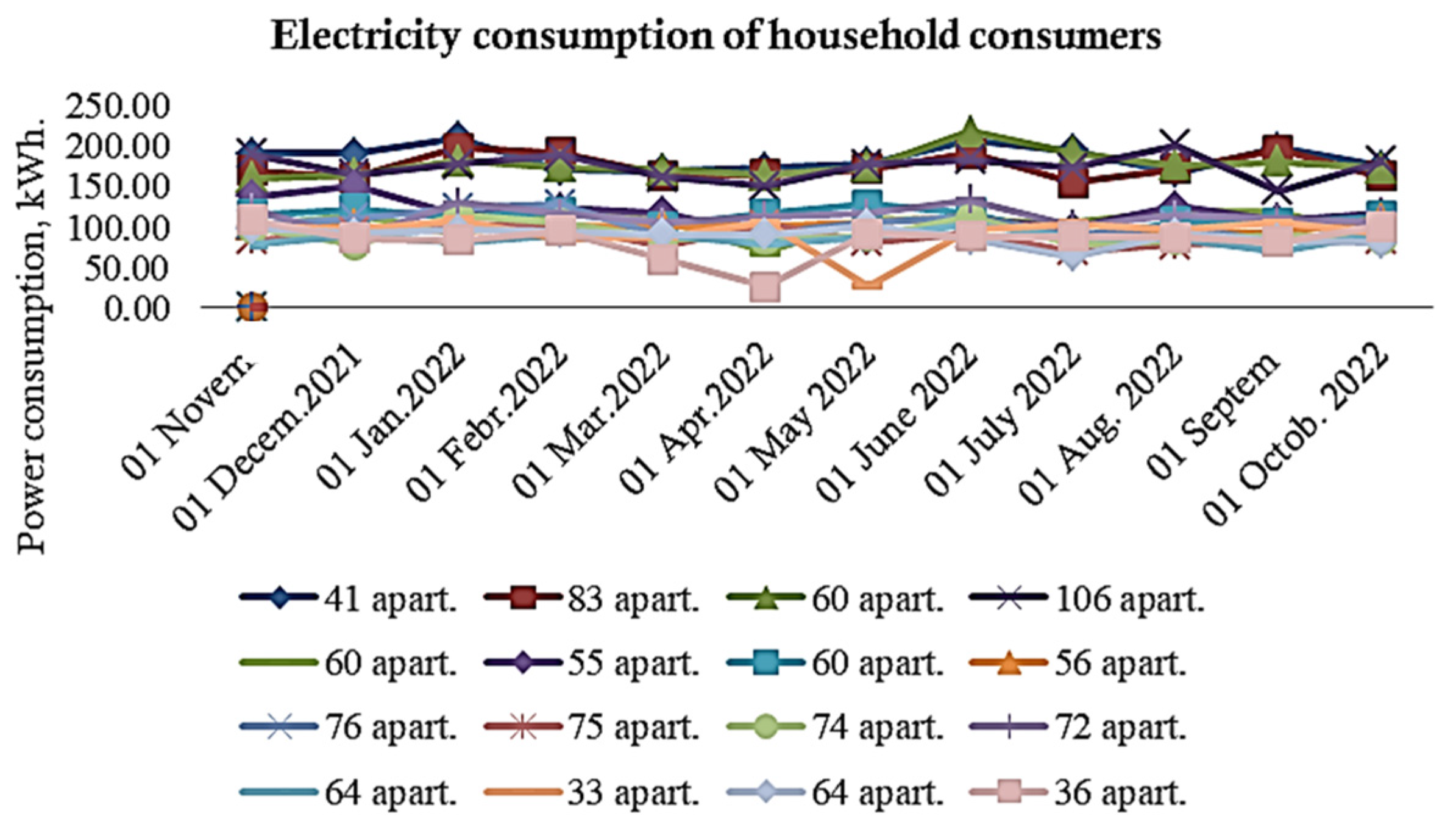
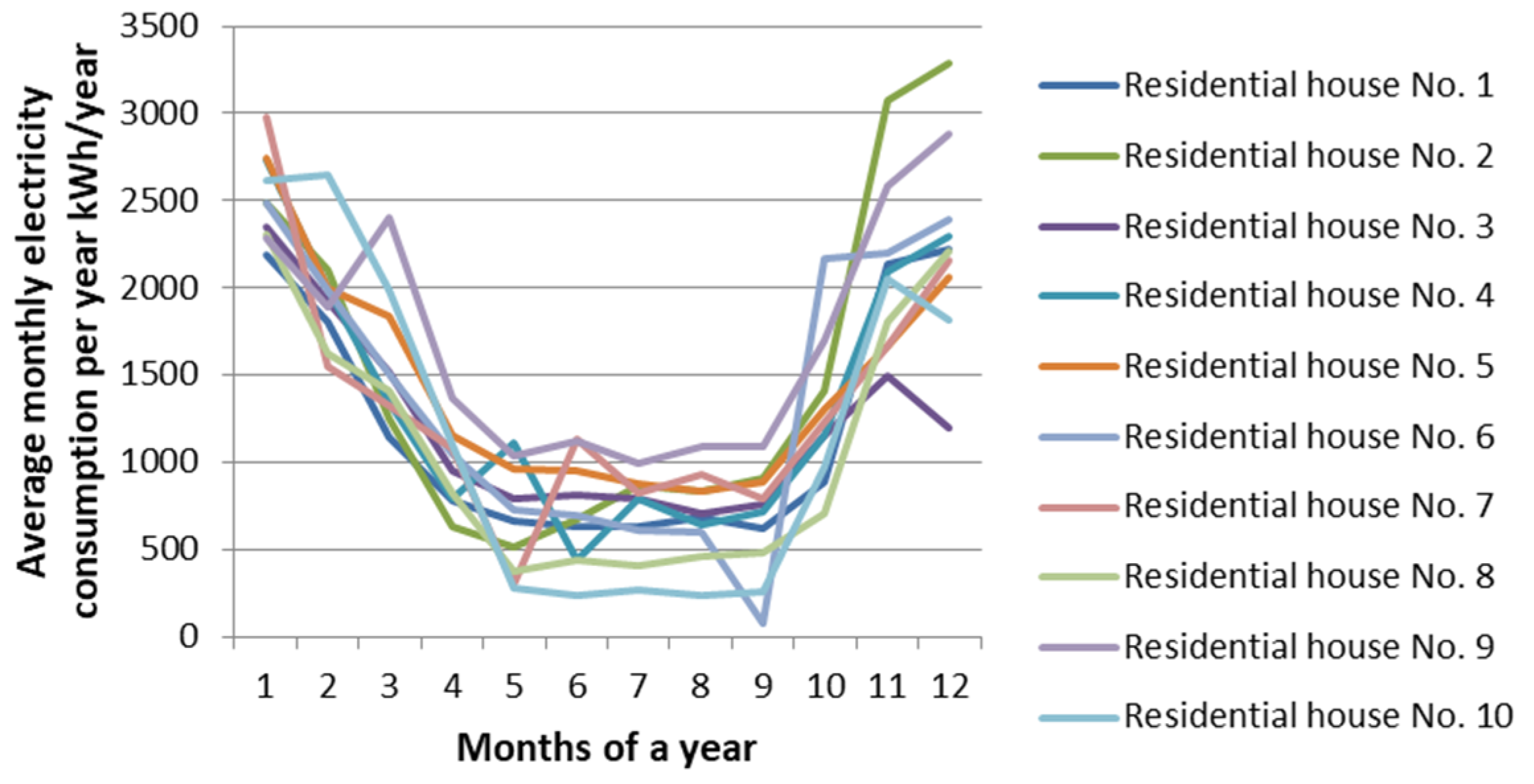
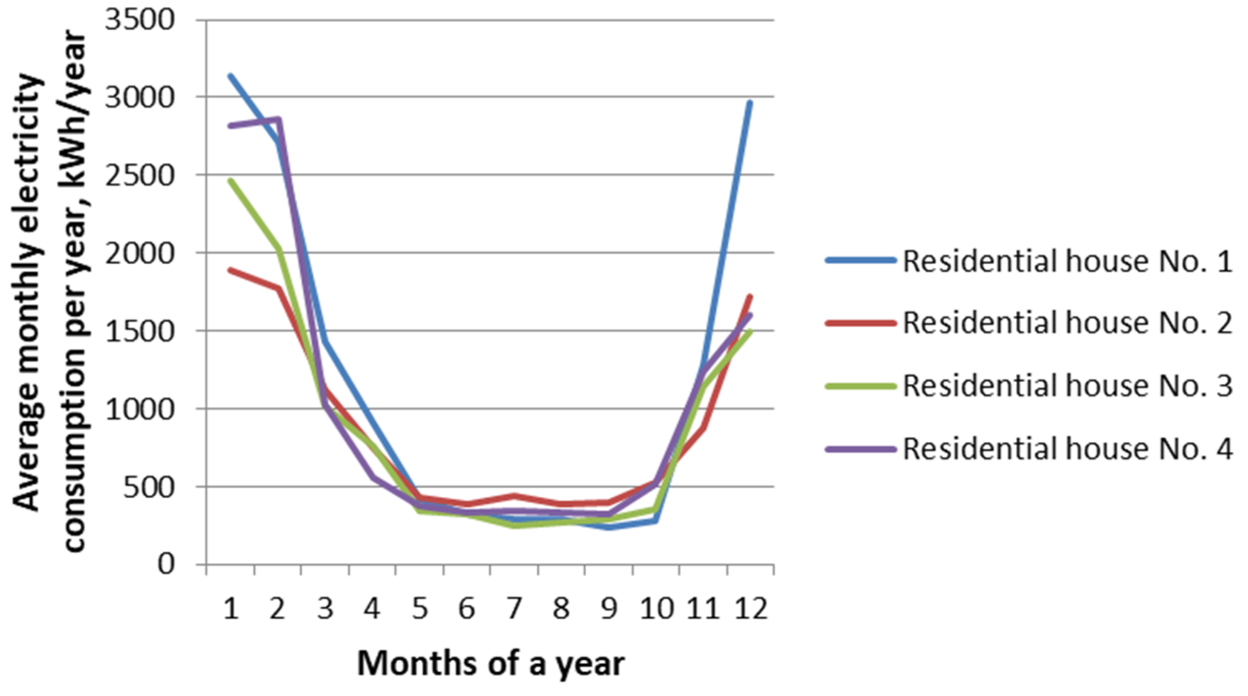
2.2. Forecasting of Power Consumption

The essence of the proposed approach is to divide meteorological conditions into m clusters using unsupervised machine learning (k-means algorithm [29]. Each cluster builds its neural network model. When the system is running, the input data refer to one of the clusters, and then the model that was built for this cluster is used to obtain the forecast.

This approach has the following advantages:

• The clustering stage is performed as unsupervised learning, meaning that the risk of fitting to the desired result is excluded;
• The consistency of the clustering result can be checked visually by applying the PCA after clustering and visualizing the resulting clusters using a scatter plot;
• The construction of different models for individual meteorological factors allows for an increase in the accuracy of the forecast since each model is focused on certain operating conditions;
• Individual models may be more compact than a single one; therefore, fewer data can be used for their training and testing, and their work will be more predictable.

On the basis of previous studies, factors were identified [30], the generalization of which made it possible to propose an A coefficient that takes into account household consumers who receive power from both combined sources (traditional (T)) and single sources (for example, completely from renewable energy sources—hydraulic, solar, wind, etc.), (E).

$${\mathrm{A}}_{\mathrm{i}\left(\mathrm{T}\right)}=(t_{i}h+c)/(s+k),$$

(5)

$${\mathrm{A}}_{\mathrm{i}\left(\mathrm{E}\right)}=\left(t_i·h·c\right)/(s·k)$$

(6)

where t_i—the temperature coefficient (taking into account the territorial–meteorological factor);

h—a coefficient that takes into account the location of consumers above sea level;

c—the coefficient that takes into account the structural design of the residential building;

s—the coefficient of the material (financial) well-being of the consumer (consumer welfare is an analogue of the income of the Törnqvist function, taken in the range from 0 to 1). The growth of this coefficient indicates the consumer’s ability to use the maximum number of household electric receivers; k is a coefficient that takes into account the dynamics of the consumer’s welfare (a different number of electric receivers for abnormal electricity consumers).

The denominators of Equations (5) and (6) allow us to establish the influence of other energy sources (except electric) on electricity consumption and electric loads. In the denominators of the product, the significance of the absence of other energy sources (heat and hot water supply and gas supply) for consumers will greatly influence the value of the expected (predicted) electric load. Therefore, the resulting value of the proposed generalized coefficient A will decrease. Whereas, with the sum in the denominators, the value of the expected (predicted) electric load will not depend so much on electric energy because during peak hours, due to the presence of other energy sources for consumers, the total consumption of electricity will decrease.

The temperature coefficient $t_i$ is determined depending on the ambient temperature at the consumer’s location:

$$t_i={\displaystyle \frac{\left|t_1\right|-\left|t_2\right|}{t_3}},$$

(7)

where t₁—the average daily temperature of the object of study, °C;

t₂—the additional temperature (the difference between the optimal and permissible temperature in the apartment), °C;

t₃—the average daily temperature at sea level.

The coefficient, taking into account the difference in altitude above sea level, is thus determined:

$$h={\displaystyle \frac{\left|t_1\right|}{{|t}_3|}}.$$

(8)

The coefficient of the structural design of buildings and premises is therefore

$$c={\displaystyle \frac{\left|t_1\right|}{t_4}},$$

(9)

where t₄—the optimal temperature in apartments, °C.

The developed generalized coefficient A_i in combination with the data of the average monthly electricity consumption makes it possible to determine the average daily electric load of apartments in apartment buildings and private housing construction. Next, we present the formula for the average daily calculation of electric power taking into account the generalized coefficient A_i:

$$P_{averagem}={\displaystyle \frac{W_{\left(averagem\right)}}{(N_d·T_{day}·{\mathrm{A}}_{\mathrm{i}})}},$$

(10)

where $W_{\left(averagem\right)}$—the average monthly electricity consumption of apartments, kWh;

$T_{day}$—the duration of the time of day, in hours;

$N_d$—the number of days in the month;

A_i—the generalized coefficient.

To determine the electrical load during maximum hours, taking into account the proposed generalized coefficient ${\mathrm{A}}_{\mathrm{i}\left(\mathrm{E}\right)}$ and the maximum load time coefficient under conditions with a single energy source [28], we propose using the following equation:

$$P_{m.l.t.}={\displaystyle \frac{W_{\left(averagem\right)}}{(N_d·T_{day}·{\mathrm{A}}_{\mathrm{i}\left(\mathrm{E}\right)}·{\alpha }_{m.l.t})}},$$

(11)

where ${\alpha }_{m.l.t}$—the maximum load time coefficient.

As you know, the hours of maximum load are observed in winter (the so-called morning and evening maximum). To derive a coefficient characterizing the maximum electricity consumption on the basis of long-term observation of the estimated time of maximum load, 6 h were taken for Dushanbe, and 7 h per day for the cities of the Gorno-Badakhshan Autonomous Region, Khorog [30].

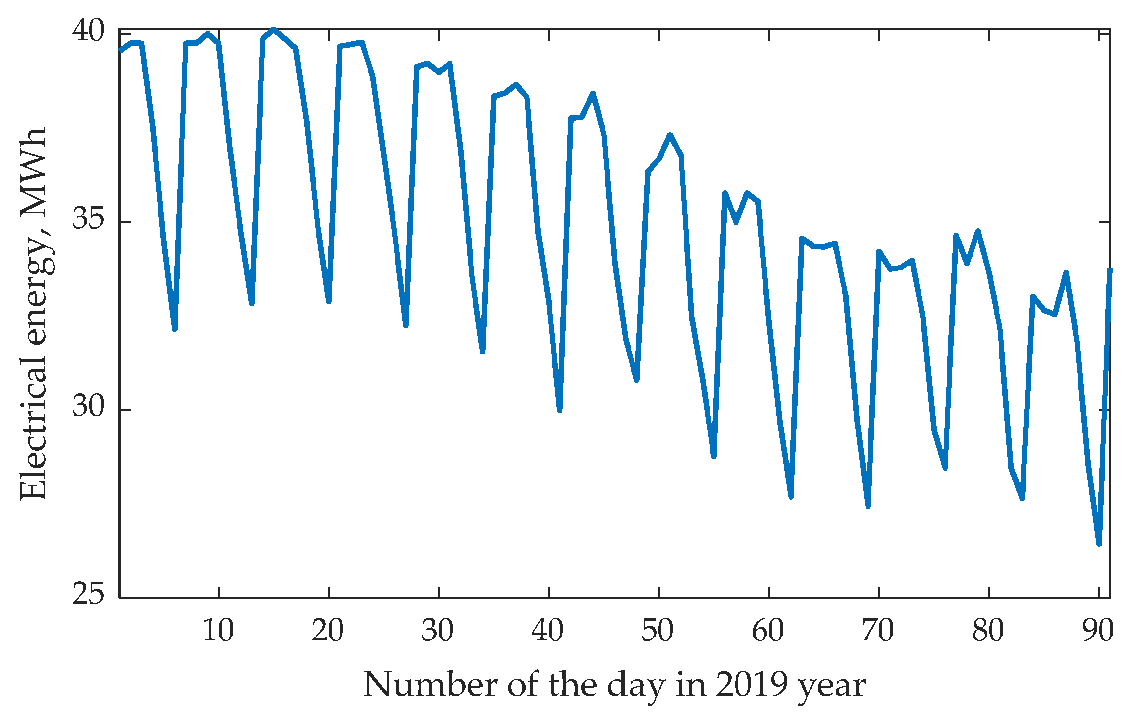
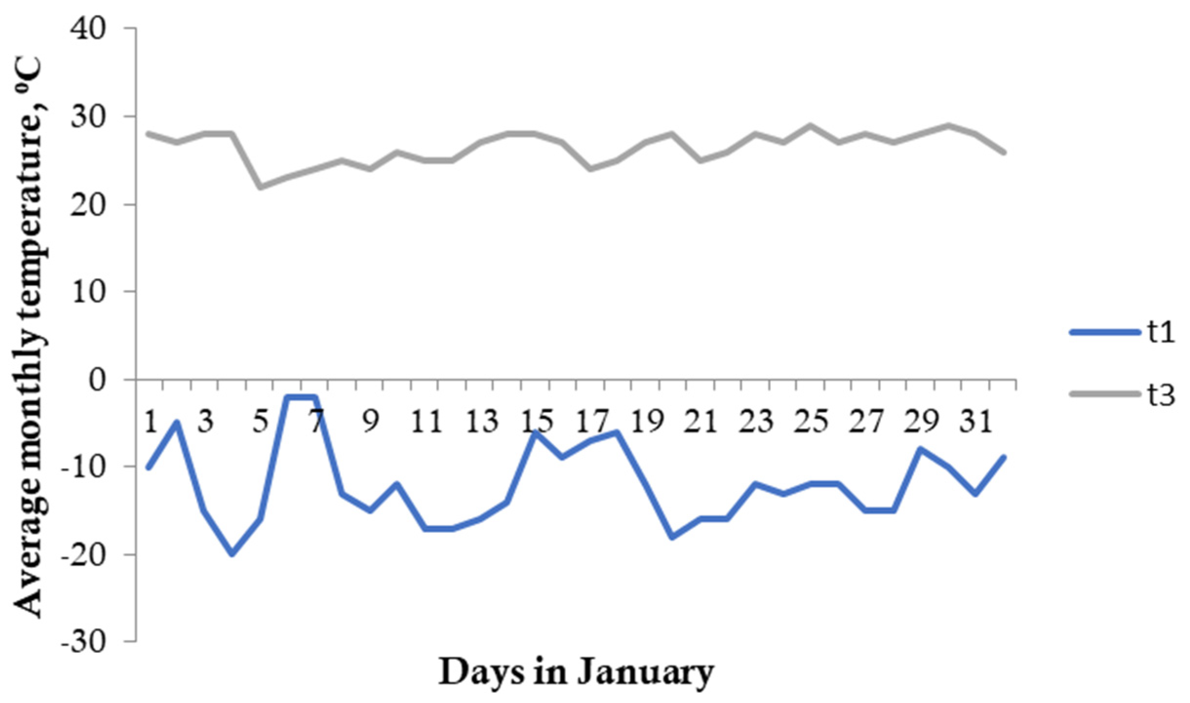
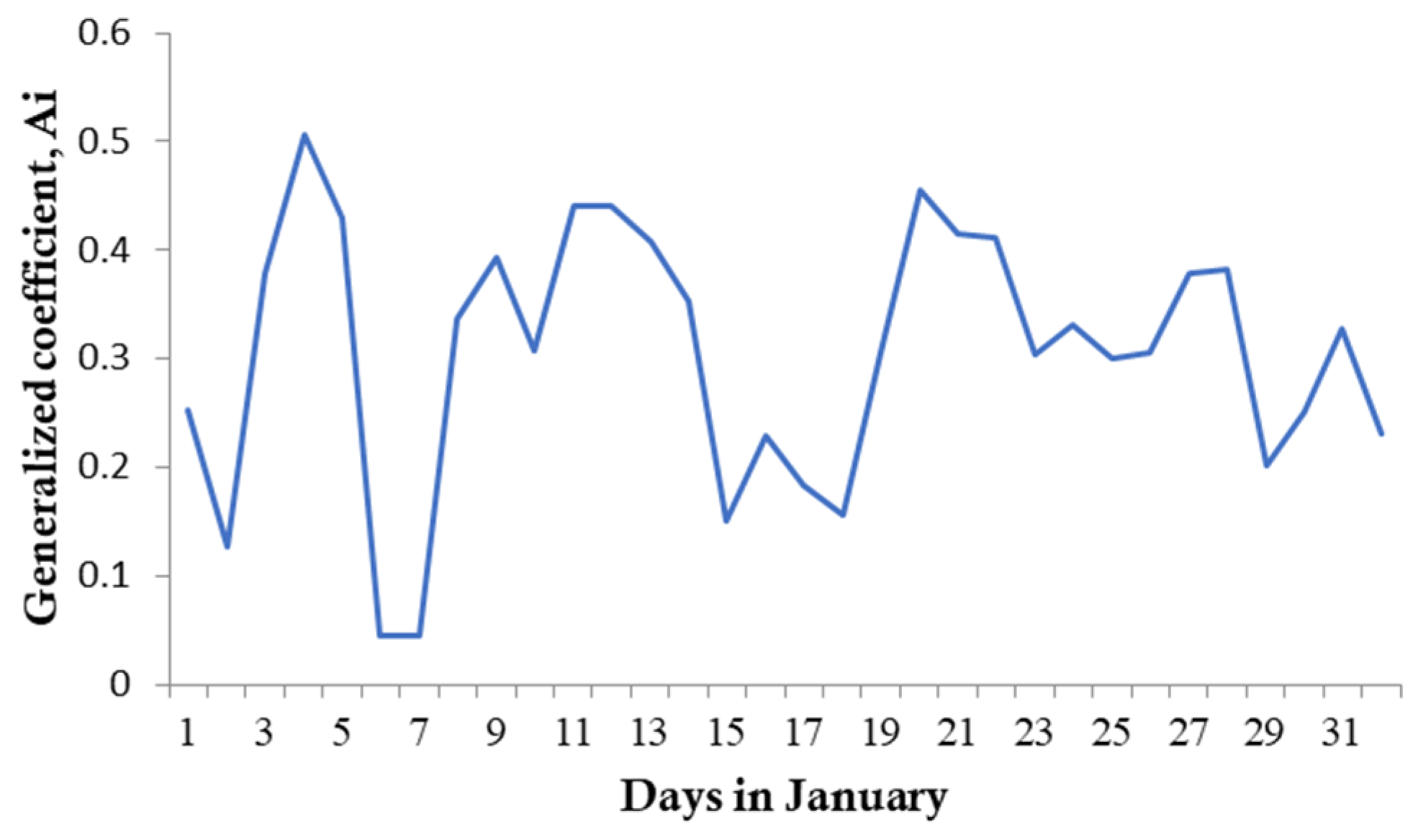
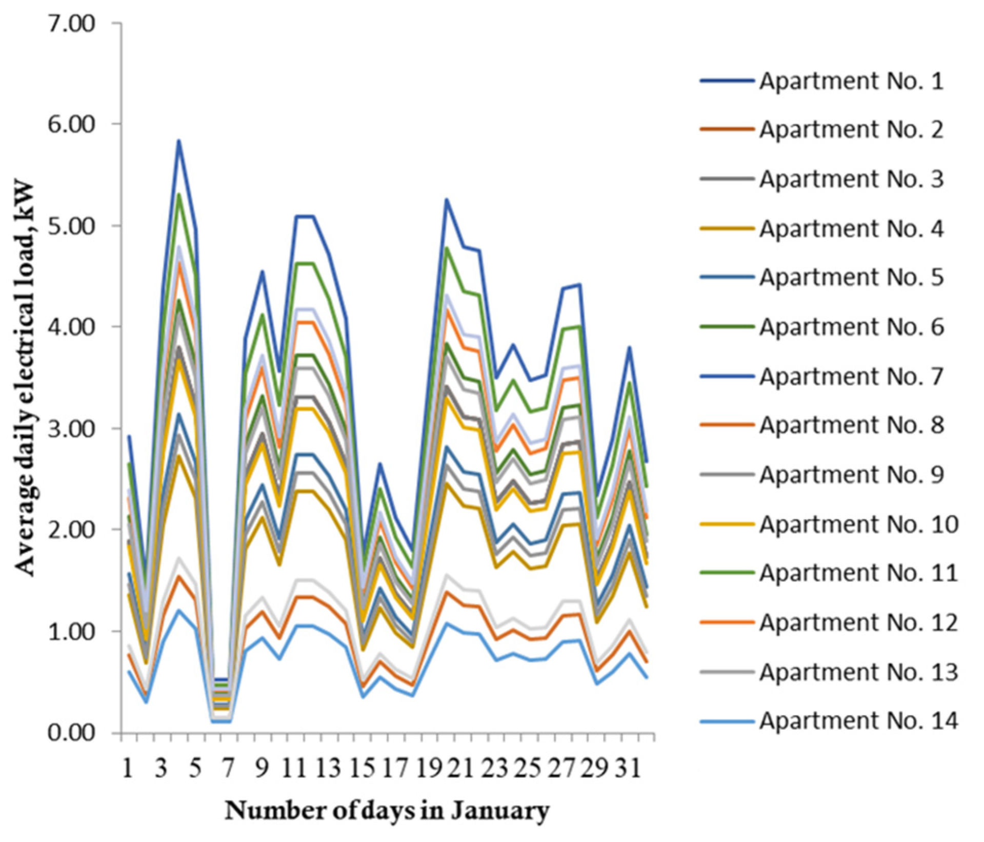
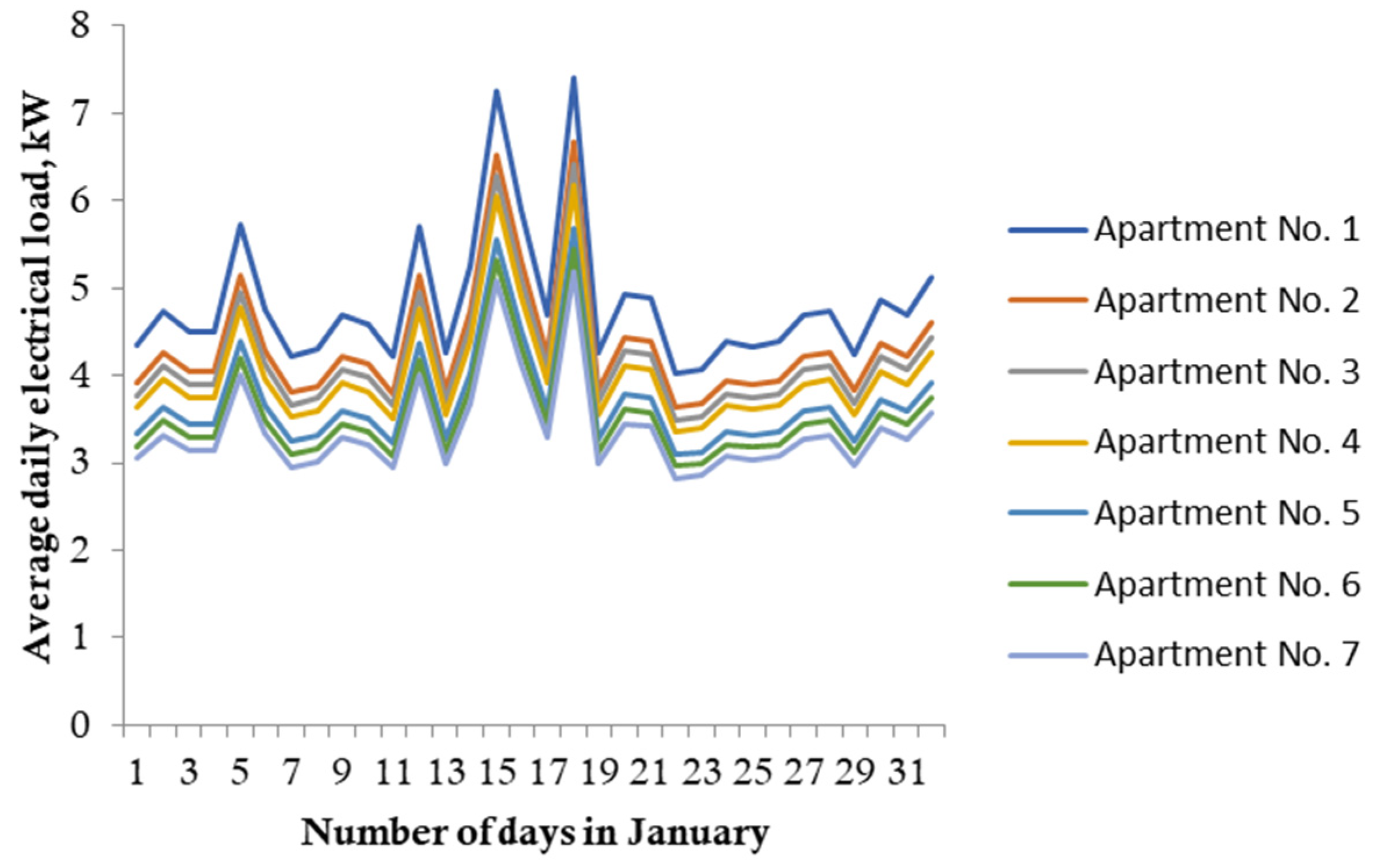
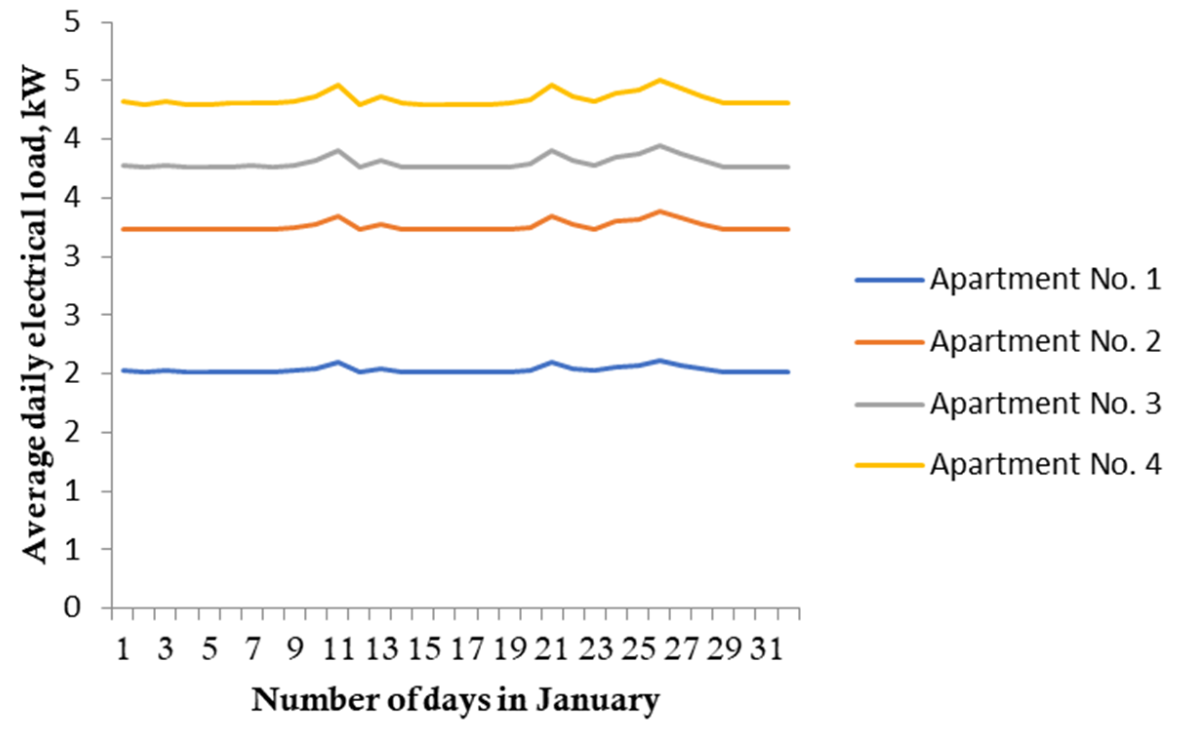
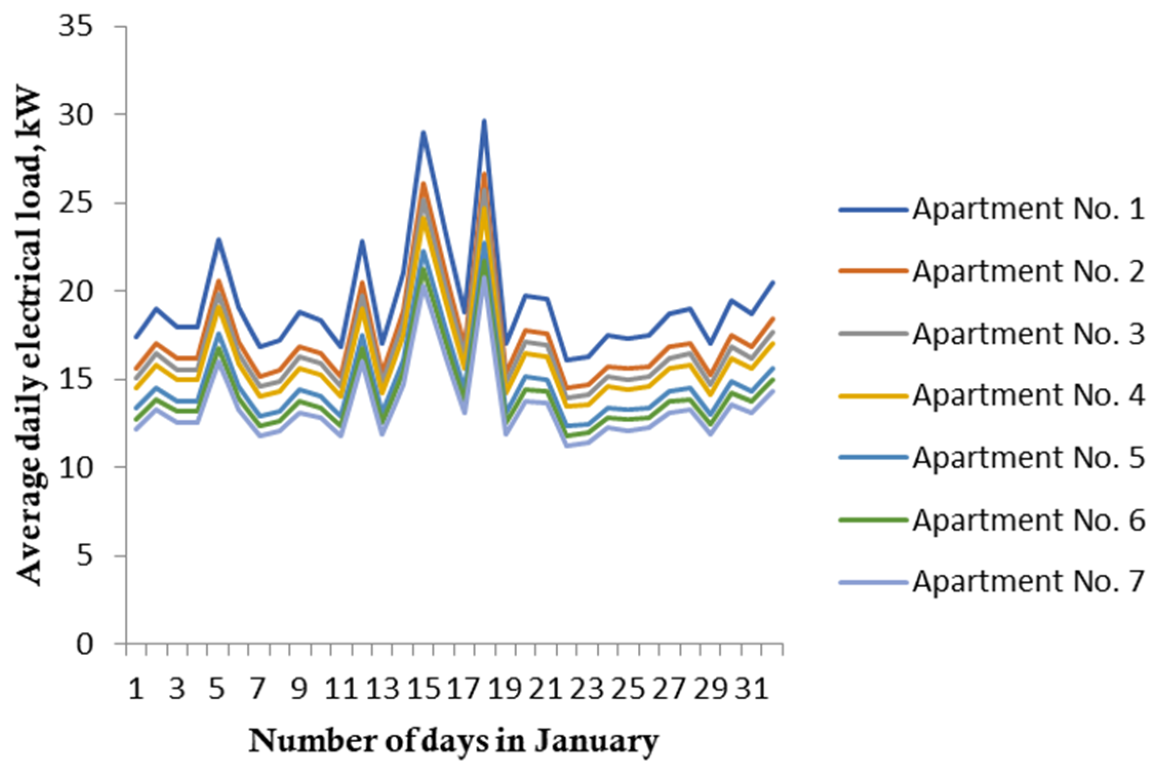
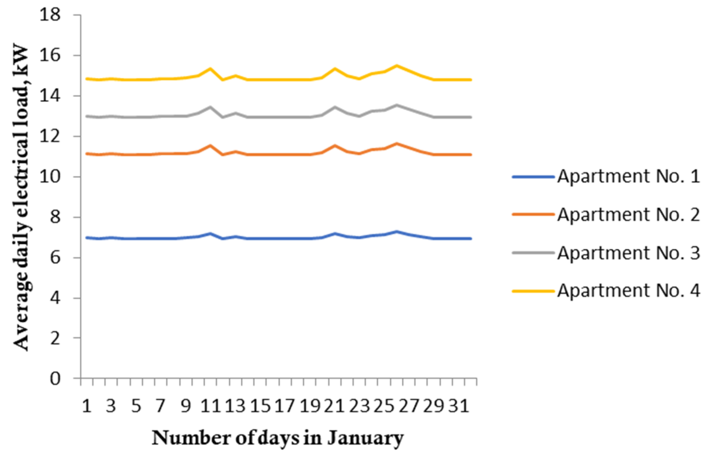
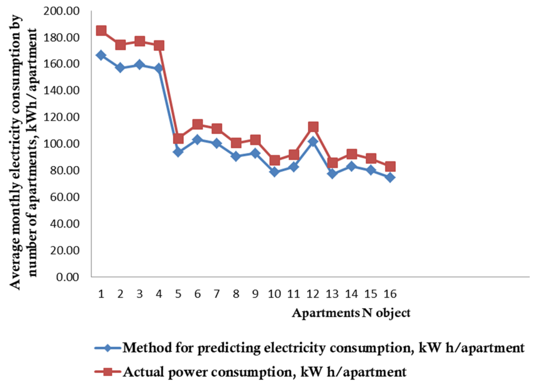
3. Electrical Load Forecasting

Since the shortage of electricity generated by the HPP is observed during the cold period from November to March, only data for these five months are considered.

The main hypothesis of this study is the possibility of increasing the accuracy of medium-term forecasting of electrical consumption through the use of meteorological data.

In addition, the load changes on weekends in the examined power system; thus, the number of days of the week are added to the dataset. The numbers of the year, month, and day are also considered features. A complete list of features in the original dataset is as follows: year, month, day, day of the week, air temperature, relative humidity, wind speed, and cloud cover. For instance, profiles of consumption changes are given below in Figure 1 and Figure 2. The correlation coefficients between features and power consumption are shown in

Table 1. The correlation coefficient between features and power consumption.

Feature	Correlation Coefficient
Year	0.70
Month	−0.09
Day	0.01
Day of the week	−0.51
Temperature	−0.33
Humidity	0.20
Wind speed	−0.37
Cloud cover	0.01

.

Power consumption (average daily load capacity) is the target variable. The dataset contains records for six years (2015–2020) in one-day increments. Thus, the dataset contains 908 rows and 9 columns.

It can be seen that the greatest dependence is observed between power consumption and the year (0.7) and the day of the week (0.51), and in terms of meteorological conditions, between power consumption and wind speed (0.37). The dependence on meteorological factors such as temperature, humidity, and cloud cover also affects power consumption.

Using the data obtained from the automated system for monitoring and accounting of electricity for 2021–2022, an average monthly graph of electricity consumption with averaging per apartment was constructed for the consumers of the city of Chelyabinsk of the Russian Federation, as shown in Figure 3. The reasons for choosing these cities are that they have distinctive features in accordance with their location in different territorial and meteorological areas. Consumers of the city of Chelyabinsk are provided with hot and warm water supply, while the cities of the Republic of Tajikistan have only a single energy source (electricity). However, the standard values of specific electrical loads for all the cities under consideration are the same, and the same document is used when designing power supply systems.

Using the data of average monthly electricity consumption for 226 apartments in ABs (Figure 4) and 7 individual housing construction (Figure 5) for 2022 (obtained from the power supply organization of Chelyabinsk and for the most typical cities), according to the criteria—that is, the territorial and meteorological factors of the Republic of Tajikistan (location of ABs above sea level and climatic factors)—the average daily electric loads for the month of January were calculated (Figure 6 and Figure 7).

Using the example of one apartment, we will present the sequence used to calculate the average daily electric load, taking into account the generalized coefficient of ${\mathrm{A}}_{\mathrm{i}\left(\mathrm{T}\right)},$ for the city of Chelyabinsk.

(1) Determination of the temperature coefficient $t_i$. For this purpose, the average daily temperature of the object of study (apartment) $t_1$ for January 2022 and the average daily temperature at sea level $t_3$ were obtained from archival data (Internet). The results are presented in the form of Figure 8 for the city of Chelyabinsk and Figure 9 for the cities of Dushanbe and Khorog of the Republic of Tajikistan (RT).

Substituting the results given in Figure 8 in Equation (7), we can determine the temperature coefficient—$t_i$ for the 1st day of January 2022 in one apartment:

$${\mathrm{t}}_{\mathrm{i}}={\displaystyle \frac{\left|-10\right|-\left|(-10-18+22)\right|}{28}}=0.14$$

(2) Using Equation (8), we calculate the coefficient for taking into account the difference in altitude above sea level:

$$\mathrm{h}={\displaystyle \frac{|-10|}{\left|28\right|}}=0.36$$

(3) Using Equation (9), we calculate the coefficient of the structural design of buildings and premises:

$$\mathrm{c}={\displaystyle \frac{|-10|}{22}}=0.45$$

(4) Substituting the results of calculating the coefficients ($t_i$, h and c) into Equation (5), we obtain

$${\mathrm{A}}_{\mathrm{i}}={\displaystyle \frac{0.14·0.36+0.45}{1+1}}=0.25.$$

(5) By substituting the result of the generalized ${\mathrm{A}}_{\mathrm{i}}$ coefficient into formula 10, we determine the average daily load of one apartment:

$$P_{averagem}={\displaystyle \frac{180}{(31·24·0.25)}}=0.96\mathrm{k}\mathrm{W}.$$

Similarly, for other days (January 2022), a generalized coefficient of ${\mathrm{A}}_{\mathrm{i}}$ was calculated. The results are presented in the form of Figure 10 for Chelyabinsk.

Based on the average monthly electricity consumption data presented in Figure 4 and the values of the generalized coefficient ${\mathrm{A}}_{\mathrm{i}}$ (see Figure 10), we present the values of changes in the electric load by day (January 2022) (Figure 11) and for private housing construction (Figure 12) for the city of Chelyabinsk and for Dushanbe (Figure 13) and Khorog (Figure 14), Republic of Tajikistan.

As can be seen from the above results of calculating the average daily electric load (Figure 11, Figure 12, Figure 13 and Figure 14), the value of the actual power is below the SEL. However, the value of the actual capacity of the cities of Dushanbe and Khorog in relation to the city of Chelyabinsk is two times higher. This once again confirms that the lack of other energy sources is the reason for the increase in electricity consumption due to the increase in the number of connected electricity receivers in households.

Further, using Equation (11) and according to the data of average monthly electricity consumption (Figure 6 and Figure 7), taking into account the obtained maximum load time coefficient and the generalized coefficient ${\mathrm{A}}_{\mathrm{i}\left(\mathrm{E}\right)}$, changes in the electric load during the maximum hours for the days of apartments in the AB were calculated and averaged per apartment in Dushanbe and Khorog. The results are presented in the form of Figure 15 and Figure 16.

As can be seen, the results of modeling the average daily load for apartments in apartment buildings and private housing construction based on the data of average monthly electricity consumption, taking into account the generalized coefficient of ${\mathrm{A}}_{\mathrm{i}\left(\mathrm{E}\right)}$ for the city of Chelyabinsk and the cities of the Republic of Tajikistan, show that the actual capacity is lower than the installed SEL.

In turn, the simulation results showed a high convergence with the results previously obtained on the basis of measurements for the city of Chelyabinsk [30]. However, due to the lack of other energy sources (gas supply and hot water supply) in the conditions of the Republic of Tajikistan and on the basis of the obtained maximum load time factor [28,30] and the generalized coefficient ${\mathrm{A}}_{\mathrm{i}\left(\mathrm{E}\right)}$, the obtained values of actual capacity exceed the maximum in hours by 1.2–2.5 times the SEL of the given RB 256.1325800.2016.

This, in turn, creates the prerequisites for disruption of the operating mode of the elements of the 6–10/0.4 kV distribution electric network, which will undoubtedly lead to a violation not only of the requirements of NS R 12.1.038-2024 but also of the service life of the elements of the urban distribution electric network.

The results of determining the electric load based on the data of the average monthly electricity consumption and the developed generalized coefficient of ${\mathrm{A}}_{\mathrm{i}}$ obtained on the basis of the proposed scheme showed that consumers of electricity (apartments) in apartment buildings and private housing construction for the considered city of Chelyabinsk and cities of the Republic of Tajikistan are lower than the SEL. Whereas, in the hours of maximum load in the AB of the cities of the Republic of Tajikistan, the actual power is higher than the SEL. Thus, the approach proposed by us makes it possible to determine the electric load from the data of electricity consumption, taking into account the generalized coefficient A for apartment buildings and individual residential buildings with sufficient accuracy without carrying out a significant number of measurements.

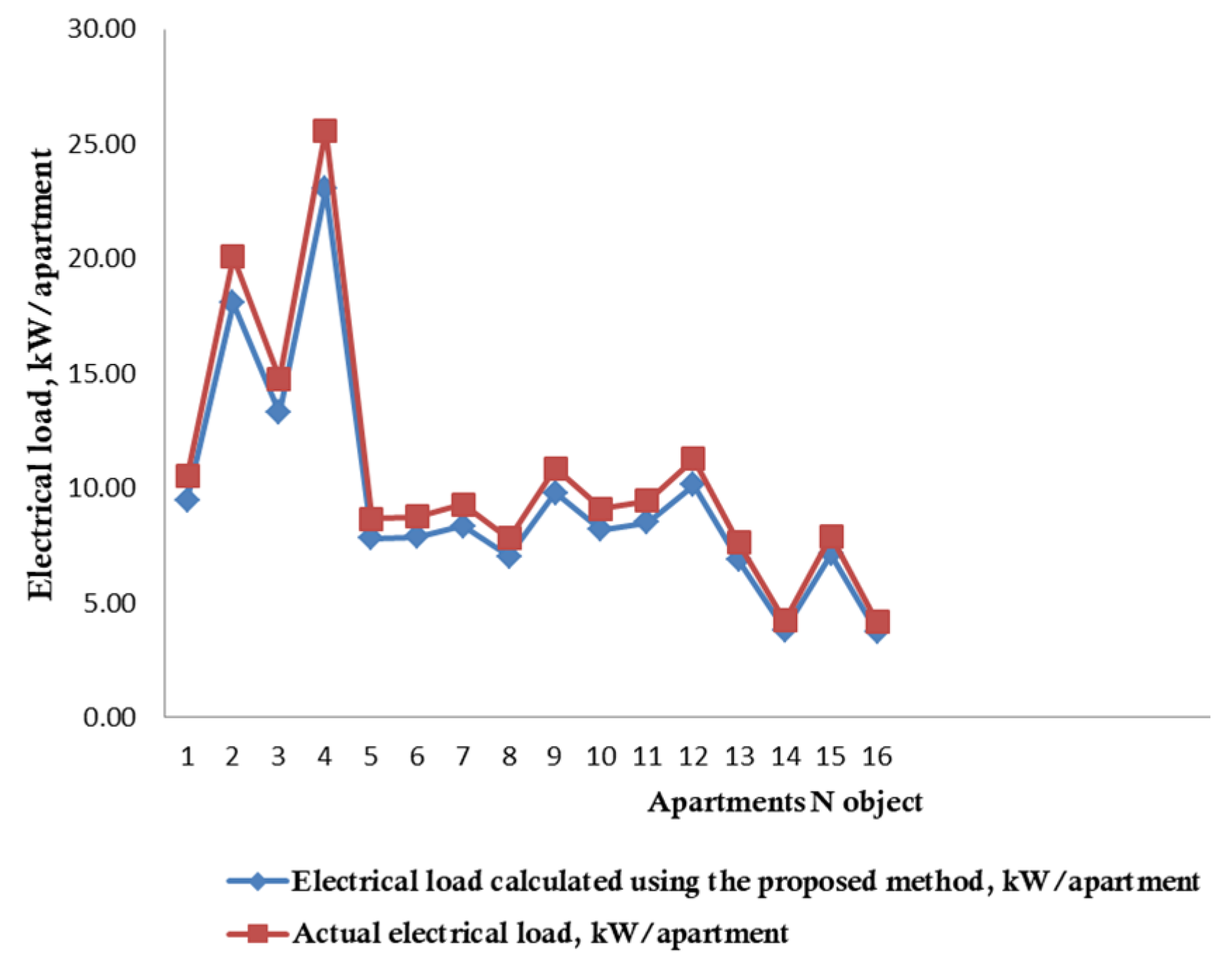
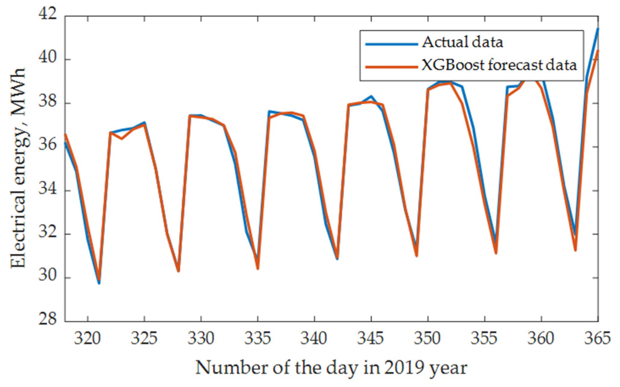
4. Comparison of Actual and Forecast Values

Using Equation (11) and based on the previous year’s data on electricity consumption by household consumers, electrical loads for the cities under consideration were calculated. The results of comparing the values obtained using the proposed method with the predicted actual values are presented in Figure 17.

According to Figure 17, the discrepancy between the predicted and actual loads did not exceed 1%.

Using the transformed Equation (10), we will predict the electricity consumption by public utilities for the cities under consideration and compare these results with the actual loads. The results of the comparison will be presented in the form of a graph (Figure 18).

Since many heterogeneous factors are used, an ANN is chosen as the basic method for constructing a regression model. The dataset is not large enough to use more complex architectures such as convolutional or recurrent neural networks. Therefore, a multilayer perceptron with the following elements is used:

• An input layer;
• A hidden layer of 32 neurons with ReLU activation function;
• A hidden layer of 16 neurons with ReLU activation function;
• A hidden layer of 8 neurons with ReLU activation function;
• An output neuron with a sigmoidal activation function.

The training is performed using the Adam algorithm [29]. The model is implemented using Python 3.6, libraries such as Keras and TensorFlow.

The proposed approach is compared with a single ANN model (excluding clusters), an AR model that does not use meteorological data, an LR that uses meteorological data, RF, and XGBoost.

The use of clustering by meteorological conditions increases the accuracy for LR, ANN, RF, and XGBoost. The error reduction was from 1.02 MW to 0.84 MW (18%) for ANN; from 0.77 MW to 0.58 MW (25%) for LR; from 1.24 MW to 0.44 MW (65%) for RF; and from 0.74 to 0.32 (57%) for XGB. At the same time, if the number of clusters is more than optimal, there may be a reverse effect, since there will be not enough data in each of the clusters to train the model. The highest forecasting accuracy was obtained using XGBoost model when dividing the data into three clusters.

Figure 19 shows the impact of clustering.

The use of meteorological conditions reduces the forecast error; the error difference between the AR model that does not use meteorological parameters and the mathematically closest model (linear regression) using these parameters was 0.22 MW (27%). The significant advantage of LR over ANN models was somewhat unexpected. This output could be explained by two factors:

• The use of features obtained using PCA as additional input features, which made it possible to aggregate meteorological factors in many ways even before the use of regression models.
• The amount of data, which was not large enough for the effective use of neural networks; their more efficient operation probably requires data for 10–20 years.

The MAE on the test part of the dataset is 0.32 MW, the root mean squared error (RMSE) is 0.39 MW, and the MAPE is 2.98%. Compared with the autoregression model without clustering and taking into account meteorological factors (MAE 0.80 MW, RMSE 0.96 MW, MAPE 6.11%), this can, according to preliminary estimates, lead to an average decrease in the generation capacity of DPP by 0.5 MW or 12 MWh per day. It should be emphasized that the result obtained makes it possible to create a reliable and very simple model based on machine learning whilst only making minimal use of complex and poorly controlled machine learning methods.

Figure 20 shows a comparison between the true and the forecast load plot for one fragment of the test set.

5. Conclusions

A method for calculating the electrical loads of apartment buildings has been developed using the developed generalized coefficient ${\mathrm{A}}_{\mathrm{i}}$. Based on average monthly electricity consumption data, it allows us to determine the compliance of the actual power with the specific power without long-term measurements. To determine the actual electrical power of apartment building loads during peak load hours with single sources, a maximum load coefficient has been proposed for the first time based on the justification for cities in the Republic of Tajikistan with different territorial and meteorological factors. Using the improved method for calculating the actual electrical power, it has been shown that in apartment buildings and individual housing construction in the city of Chelyabinsk and cities in the Republic of Tajikistan, the actual power is lower than the specific power, while during peak load hours in apartment buildings in cities in the Republic of Tajikistan, the actual power is higher than the specific electrical loads. Based on the developed method for forecasting apartment building electricity consumption under uncertain conditions, temporary electricity consumption standards will be proposed for cities in the Republic of Tajikistan in the future.

References

1. Blazakis, K.V.; Kapetanakis, T.N.; Stavrakakis, G.S. Effective Electricity Theft Detection in Power Distribution Grids Using an Adaptive Neuro Fuzzy Inference System. Energies 2020, 13, 3110. [Google Scholar] [CrossRef]
2. Issi, F.; Kaplan, O. The Determination of Load Profiles and Power Consumptions of Home Appliances. Energies 2018, 11, 607. [Google Scholar] [CrossRef]
3. Ziel, F. Load Nowcasting: Predicting Actuals with Limited Data. Energies 2020, 13, 1443. [Google Scholar] [CrossRef]
4. Foltyn, L.; Vysocký, J.; Prettico, G.; Běloch, M.; Praks, P.; Fulli, G. OPF solution for a real Czech urban meshed distribution network using a genetic algorithm. Sustain. Energy Grids Netw. 2021, 26, 100437. [Google Scholar] [CrossRef]
5. Ahmad, A.; Javaid, N.; Mateen, A.; Awais, M.; Khan, Z.A. Short-Term Load Forecasting in Smart Grids: An Intelligent Modular Approach. Energies 2019, 12, 164. [Google Scholar] [CrossRef]
6. Ahmed, R.; Sreeram, V.; Mishra, Y.; Arif, M.D. A review and evaluation of the state-of-the-art in PV solar power forecasting: Techniques and optimization. Renew. Sustain. Energy Rev. 2020, 124, 109792. [Google Scholar] [CrossRef]
7. Angelini, G.; De Angelis, L. Efficiency of online football betting markets. Int. J. Forecast. 2019, 35, 712–721. [Google Scholar] [CrossRef]
8. Apiletti, D.; Pastor, E. Correlating espresso quality with coffee-machine parameters by means of association rule mining. Electronics 2020, 9, 100. [Google Scholar] [CrossRef]
9. Asimakopoulos, S.; Paredes, J.; Warmedinger, T. Real-time fiscal forecasting using mixed-frequency data. Scand. J. Econ. 2020, 122, 369–390. [Google Scholar] [CrossRef]
10. Babai, M.; Dallery, Y.; Boubaker, S.; Kalai, R. A new method to forecast intermittent demand in the presence of inventory obsolescence. Int. J. Prod. Econ. 2019, 209, 30–41. [Google Scholar] [CrossRef]
11. Barker, J. Machine learning in M4: What makes a good unstructured model? Int. J. Forecast. 2020, 36, 150–155. [Google Scholar] [CrossRef]
12. Boylan, J.; Syntetos, A. Intermittent Demand Forecasting—Context, Methods and Applications; Wiley: Hoboken, NJ, USA, 2021. [Google Scholar] [CrossRef]
13. Burton, J.W.; Stein, M.; Jensen, T.B. A systematic review of algorithm aversion in augmented decision making. J. Behav. Decis. Mak. 2020, 33, 220–239. [Google Scholar] [CrossRef]
14. Chan, F.; Pauwels, L.L. Some theoretical results on forecast combinations. Int. J. Forecast. 2018, 34, 64–74. [Google Scholar] [CrossRef]
15. Choudhury, A.; Urena, E. Forecasting hourly emergency department arrival using time series analysis. Br. J. Heal. Manag. 2020, 26, 34–43. [Google Scholar] [CrossRef]
16. Diebold, F.X.; Shin, M. Machine learning for regularized survey forecast combination: Partially-egalitarian lasso and its derivatives. Int. J. Forecast. 2019, 35, 1679–1691. [Google Scholar] [CrossRef]
17. Sergeev, N.N.; Matrenin, P.V. Enhancing Efficiency of Ensemble Machine Learning Models for Short-Term Load Forecasting through Feature Selection. In Proceedings of the 2022 IEEE 23rd International Conference of Young Professionals in Electron Devices and Materials (EDM), Altai, Russia, 30 June–4 July 2022; IEEE: Washington, DC, USA, 2022; pp. 368–371. [Google Scholar]
18. Fan, Y.; Nowaczyk, S.; Rögnvaldsson, T. Transfer learning for remaining useful life prediction based on consensus self-organizing models. Reliab. Eng. Syst. Saf. 2020, 203, 107098. [Google Scholar] [CrossRef]
19. Fezzi, C.; Mosetti, L. Size matters: Estimation sample length and electricity price forecasting accuracy. Energy J. 2020, 41, 231–254. [Google Scholar] [CrossRef]
20. Goltsos, T.E.; Syntetos, A.A.; van der Laan, E. Forecasting for remanufacturing: The effects of serialization. J. Oper. Manag. 2019, 65, 447–467. [Google Scholar] [CrossRef]
21. Grushka-Cockayne, Y.; Jose, V.R.R. Combining prediction intervals in the M4 competition. Int. J. Forecast. 2020, 36, 178–185. [Google Scholar] [CrossRef]
22. Hewamalage, H.; Bergmeir, C.; Bandara, K. Recurrent neural networks for time series forecasting: Current status and future directions. Int. J. Forecast. 2021, 37, 388–427. [Google Scholar] [CrossRef]
23. Hong, T.; Pinson, P. Energy forecasting in the big data world. Int. J. Forecast. 2019, 35, 1387–1388. [Google Scholar] [CrossRef]
24. Senyuk, M.; Safaraliev, M.; Gulakhmadov, A.; Ahyoev, J. Application of the Conditional Optimization Method for the Synthesis of the Law of Emergency Control of a Synchronous Generator Steam Turbine Operating in a Complex-Closed Configuration Power System. Mathematics 2022, 10, 3979. [Google Scholar] [CrossRef]
25. Tavarov, S.S.; Sidorov, A.I.; Sultonov, O.O. Modelling the operating mode of the urban electrical network and developing a method for managing these modes. Math. Model. Eng. Probl. 2021, 8, 813–818. [Google Scholar] [CrossRef]
26. Shiralievich, T.S.; Ivanovic, S.A.; Mamanazarovna, S.S.; Olimovich, S.O.; Yunusov, P. Learning algorithm of artificial neural network factor forecasting power consumption of users. Bull. Electr. Eng. Informatics 2022, 11, 602–612. [Google Scholar] [CrossRef]
27. Sidorov, A.; Tavarov, S. Method for forecasting electric consumption for household users in the conditions of the Republic of Tajikistan. Int. J. Sustain. Dev. Plan. 2020, 15, 569–574. [Google Scholar] [CrossRef]
28. Ungureanu, S.; Topa, V.; Cziker, A.C. Deep Learning for Short-Term Load Forecasting-Industrial Consumer Case Study. Appl. Sci. 2021, 11, 10126. [Google Scholar] [CrossRef]
29. Grant, J.; Eltoukhy, M.; Asfour, S. Short-Term Electrical Peak Demand Forecasting in a Large Government Building Using Artificial Neural Networks. Energies 2014, 7, 1935–1953. [Google Scholar] [CrossRef]
30. Tavarov, S.S.; Zicmane, I.; Beryozkina, S.; Praveenkumar, S.; Safaraliev, M.; Shonazarova, S. Evaluation of the Operating Modes of the Urban Electric Networks in Dushanbe City, Tajikistan. Inventions 2022, 7, 107. [Google Scholar] [CrossRef]
Figure 1. Consumption graph for the period January–March 2019.
Electricity 06 00026 g001
Figure 2. Consumption graph for the period November–December 2019.
Electricity 06 00026 g002
Figure 3. Average monthly electricity consumption per apartment for the period 2021–2022.
Electricity 06 00026 g003
Figure 4. Histogram of average monthly electricity consumption for 226 apartments in an apartment building, averaged per apartment.
Electricity 06 00026 g004
Figure 5. Average monthly electricity consumption for individual residential buildings.
Electricity 06 00026 g005
Figure 6. Average monthly electricity consumption of apartments in multi-apartment buildings, averaged per one apartment in Dushanbe.
Electricity 06 00026 g006
Figure 7. Average monthly electricity consumption of apartments in multi-apartment buildings, averaged per one apartment in Khorog.
Electricity 06 00026 g007
Figure 8. Average daily temperature of the research object (apartment)− t 1 and temperature at sea level− t 3 .
Electricity 06 00026 g008
Figure 9. Average daily temperature of the objects of study (apartments) located in the territories of Dushanbe and Khorog.
Electricity 06 00026 g009
Figure 10. Results of calculation of the generalized coefficient A i for the city of Chelyabinsk.
Electricity 06 00026 g010
Figure 11. Changes in electrical load, by day, of apartments in apartment buildings, averaged per apartment in Chelyabinsk.
Electricity 06 00026 g011
Figure 12. Changes in electrical load, by day, for individual housing construction, averaged per apartment in Chelyabinsk.
Electricity 06 00026 g012
Figure 13. Changes in electrical load, by day, of apartments in apartment buildings, averaged per apartment in Dushanbe.
Electricity 06 00026 g013
Figure 14. Changes in electrical load, by day, of apartments in apartment buildings, averaged per apartment in Khorog.
Electricity 06 00026 g014
Figure 15. Changes in electrical load during peak hours, by day, of apartments in apartment buildings, averaged per apartment in Dushanbe.
Electricity 06 00026 g015
Figure 16. Changes in electrical load during peak hours for apartments in apartment buildings, averaged per apartment in Khorog.
Electricity 06 00026 g016
Figure 17. Comparison of the actual electrical load with the load obtained using the proposed method.
Electricity 06 00026 g017
Figure 18. Comparison of actual power consumption with the predicted value, found by taking into account the generalized coefficient A.
Electricity 06 00026 g018
Figure 19. Comparison of MAPE with and without clustering.
Electricity 06 00026 g019
Figure 20. Comparison of true and forecast consumption schedules of electrical energy.
Electricity 06 00026 g020