Experimental Determination of a Spoke-Type Axial-Flux Permanent Magnet Motor’s Lumped Parameters

Abstract

This study focuses on the experimental determination of the lumped parameters of a Spoke-Type Axial-Flux Permanent Magnet (STAFPM) motor. This type of motor offers high specific torque and is well-suited for transportation applications. The studied STAFPM motor uses Ferrite magnets, which are more environmentally friendly and economical than rare earth magnets. The identification of the lumped electromechanical model parameters is carried out using static torque measurements on a dedicated test bench. The torque measurements are performed in two stages: with and without magnets mounted in the rotor. The no-load flux is determined separately by no-load tests. Together, these tests identify the key parameters of the lumped parameter model, such as self- and mutual inductances, cogging torque, and no-load flux. These parameters are then used to complement the DQ model, commonly used in electric motor analysis. While the DQ model predicts average torque well, it cannot reproduce torque ripples. The lumped parameter model, validated by three-phase DC testing, provides an accurate representation of the motor’s behavior, including torque ripples. This study also applies Maximum Torque Per Ampere (MTPA) control strategies and offers a practical alternative to 3D Finite Element Analysis (FEA), thus aiding the design of STAFPM motors.

1. Introduction

This article deals with Spoke-Type Axial-Flux Permanent Magnet (STAFPM) machines, which are of great interest in transportation applications [1,2]. They can provide a much higher air-gap flux density due to the flux concentration achieved by ferromagnetic pole pieces arranged between the permanent magnets at the rotor. Thus, they can achieve extremely high specific torque [3,4], just like other permanent magnet axial-flux machines [5]. It is possible in the spoke-type architecture to ensure flux weakening [6,7]. One of the models most frequently used to study electric motors is the DQ model [8,9]. However, this model does not consider the effect of the torque ripples or other phenomena associated with the magnetic circuit’s geometry unless using a mixed approach with FEA [10]. The lumped parameter model, which is a more general electromechanical model of the electric motor, is therefore pertinent [11]. Experiments must be conducted to assess this model’s parameters. Since these are primarily static studies, eddy current effects can be disregarded. The estimation of the machine’s performance requires an accurate and suitable procedure to determine the lumped model’s parameters.

The torque estimation is established using a test bench that enables a precise measurement based on rotor’s position. Using various DC currents to supply the phases is one of the primary methods for calculating torque. Single-phase or double-phase current supplies are used while the rotor rotates at a constant speed [12]. The general electromechanical lumped parameter model, which is the primary foundation of this method, shows that the torque of a permanent magnet motor is equal to the sum of the electromagnetic, saliency and cogging torques [11]. Measuring torque is extremely difficult because of mechanical constraints, like resonance frequencies. Torque ripples in permanent magnet and switched reluctance motors are intended to be measured by the static torque gauge using force sensors on the rotor [13,14] or on the stator [15,16]. For the latter, they measure the reaction torque. 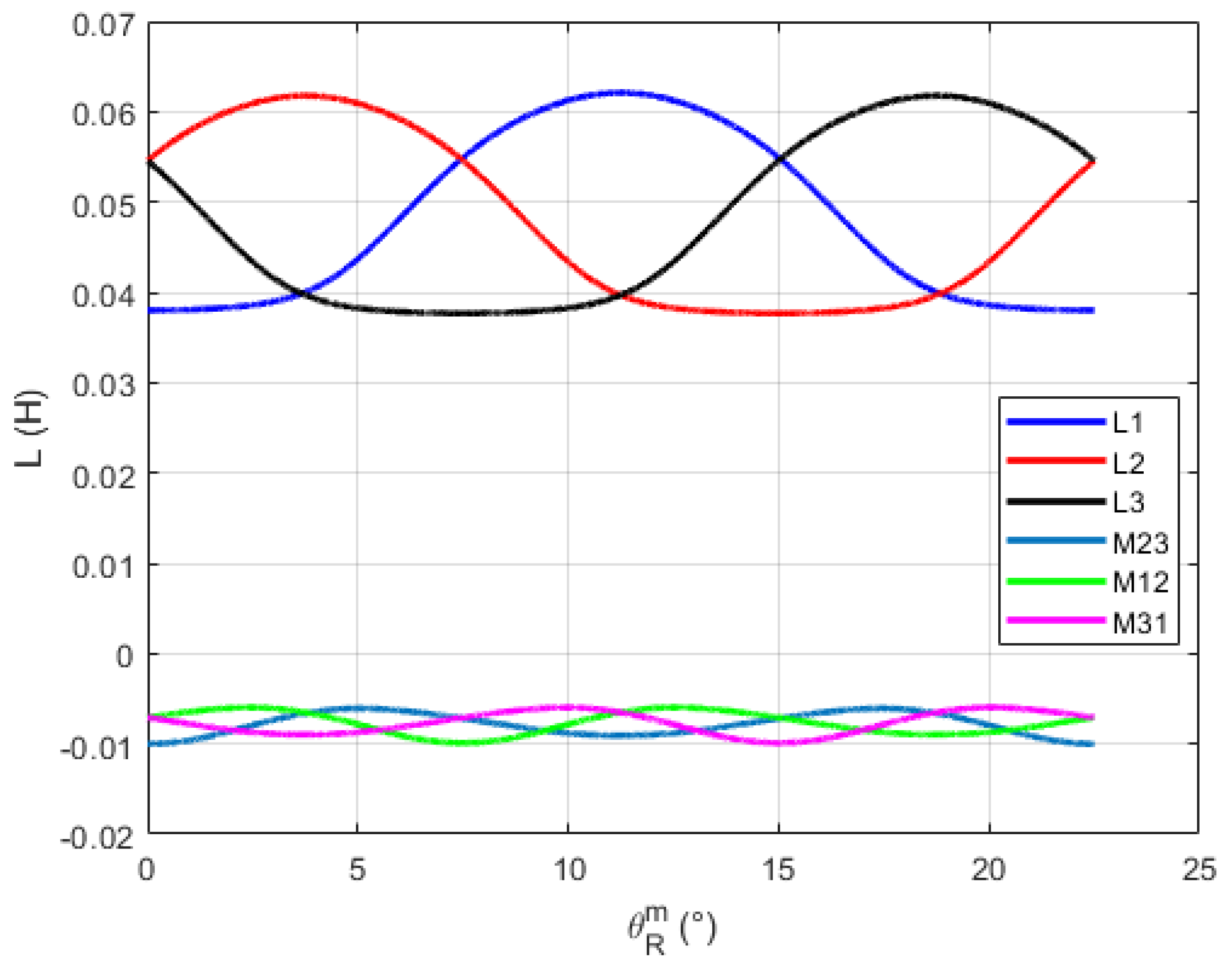The flux linkage characteristics of a switched reluctance motor were determined by Song et al., and their assumptions were confirmed through the measurement of the static torque characteristics [17]. The settlement of the self- and the mutual inductances’ harmonics as a function of rotor position are assessed in [18]. The parameters of an extended DQ model tailored to motors with non-sinusoidal waveforms are deduced using these harmonics. These parameters are then used to create a Maximum Torque Per Ampere (MTPA) control strategy for these motors in the last stage.

The aim of this article is to present the experimental investigations required to determine the parameters of the electromechanical model of a STAFPM motor produced in the laboratory [19]. This model will then enable the completion of a DQ model to examine this motor’s behavior when fed by a three-phase current system.

In Section 2 of this article, the STAFPM prototype is introduced first. In Section 3, in order to guide the experimental studies, the general electromechanical lumped parameter model is recalled. Then, physical symmetries of the motor are exploited to deduce some properties of the electromechanical parameters, such as the self- and mutual inductances and the no-load magnetic flux. These characteristics enable the establishment of procedures for determining each of the electromechanical model’s parameters. As most of the parameters can be deduced from static torques, an experimental test bench available in the laboratory is presented in Section 4. Static torque as a function of rotor position can be measured with this test bench. Section 5 presents, step by step, the identification of all the parameters of the electromechanical model. Once the general STAFPM motor model is available, it is validated in Section 6. This model makes it possible to accurately replicate several significant phenomena, including torque ripples. In Section 7, this model is used to study the motor’s three-phase sinusoidal supplies. To guide these studies, the parameters of the DQ model are calculated. Some properties of these parameters are highlighted. The optimal torque of the motor is then evaluated. In the Conclusions Section, considerations are presented on the use of the electromechanical lumped parameter model in order to size the STAFPM motor.

2. STAFPM Prototype

The STAFPM motor prototype presented in this section was developed on the basis of the stator magnet circuit of an axial-flux machine [20]. In this machine, the magnets were surface-mounted on the rotor. The rotor of our prototype was completely new to achieve a spoke-type axial-flux machine, and the stator was rewound with the correct number of winding poles. Details regarding the sizing of this motor can be found in chapter 2 of [19]. This prototype was not made for an industrial application with defined specifications. Its objective is to highlight the analysis method proposed in this article, namely the tests that must be implemented to establish the electromechanical lumped parameter model.

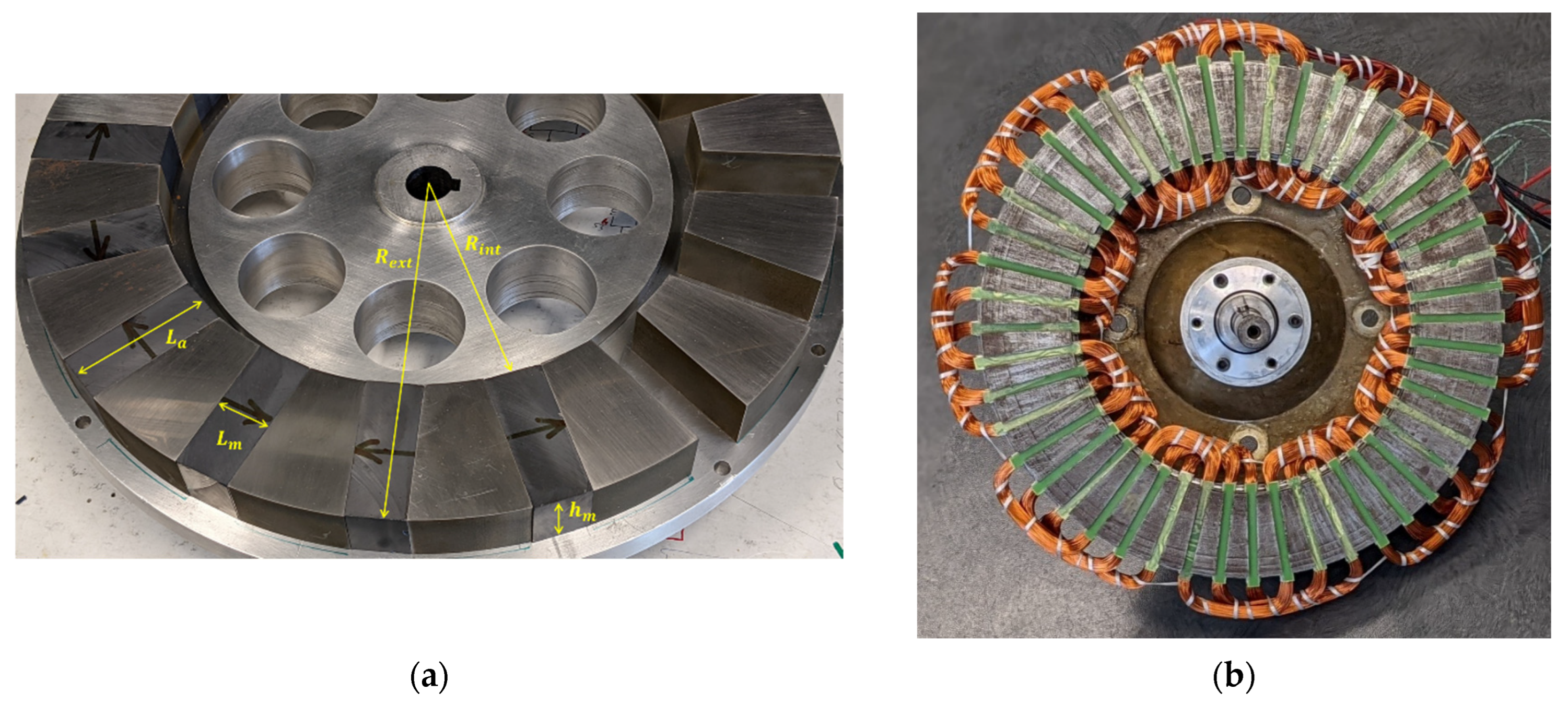
So, the STAFPM prototype is a single-rotor, single-stator, three-phase axial-flux motor. Non-oriented electrical steel of the FeSi “M235-35A” grade with a sheet thickness of 0.35 mm made up the stator’s ferromagnetic material. A ferromagnetic pole piece that concentrates the no-load magnetic flux in the air gap and an azimuthally polarized Ferrite permanent magnet constitute each rotor pole. The prototype’s Ferrite magnets have the following properties: ${\mu }_{ra}=1.1$ is the relative magnetic permeability and $J=0.37 \mathrm{T}$ is the polarization. The electrical steel XC12 served as the rotor’s ferromagnetic material. Since the total axial thickness was purposefully limited to making handling the prototype easier, the rate of concentration of the no-load magnetic flux in the air gap was equal to 1.15, which is not very strong.

Table 1. Main STAFPM prototype parameters.

Parameter	Value
$\mathrm{Number} \mathrm{of} \mathrm{phases}, q$	3
$\mathrm{Number} \mathrm{of} \mathrm{pairs} \mathrm{of} \mathrm{poles}, p$	8
$\mathrm{Number} \mathrm{of} \mathrm{slots}, n_e$	48
$\mathrm{Air-gap} \mathrm{thickness}, e_g\left(\mathrm{m}\mathrm{m}\right)$	2.0
$\mathrm{Internal} \mathrm{radius}, R_{int}\left(\mathrm{m}\mathrm{m}\right)$	100.0
$\mathrm{External} \mathrm{radius}, R_{ext}\left(\mathrm{m}\mathrm{m}\right)$	150.0
$\mathrm{Slot} \mathrm{axial} \mathrm{height}, h_{sl} \left(\mathrm{m}\mathrm{m}\right)$	12.5
$\mathrm{Stator-yoke} \mathrm{axial} \mathrm{thickness}, h_{sy} \left(\mathrm{m}\mathrm{m}\right)$	8.0
$\mathrm{Conductor} \mathrm{diameter}, d_c \left(\mathrm{m}\mathrm{m}\right)$	0.63
$\mathrm{PM} \mathrm{axial} \mathrm{thickness}, h_m \left(\mathrm{m}\mathrm{m}\right)$	23.8
$\mathrm{PM} \mathrm{azimuthal} \mathrm{width} \mathrm{at} \mathrm{the} \mathrm{mean} \mathrm{radius}, L_m \left(\mathrm{m}\mathrm{m}\right)$	19.6
$\mathrm{PM} \mathrm{radial} \mathrm{length}, L_a \left(mm\right)$	50.0

and Figure 1 present the dimensions and photos of the rotor and stator, respectively.

The stator had an integer distributed winding topology with one slot per pole and per phase ($n_{epp}=1$) and ninety-five conductors per slot $(n_c=95)$. All the conductors per phase were in series. In addition, the number of turns was $n_s=760$.

3. Electromechanical Lumped Parameter Model

3.1. Electrical and Mechanical Quantities

The supplied currents $\mathit{I}$ and induced fluxes $\mathsf{\Phi }$ are related to the instantaneous phase voltages $\mathit{V}$ imposed by the motor power supply as per the following equation:

$$\mathit{V}=\mathit{R}\mathit{I}+{\displaystyle \frac{d}{dt}}\mathsf{\Phi }$$

(1)

The resistance $\mathit{R}$ is a diagonal matrix, where $R_s$ being the resistance per phase.

For a permanent magnet synchronous motor, the currents and fluxes are linked by:

$$\mathsf{\Phi }\left({\theta }_R^e\right)={\mathsf{\Phi }}_{\mathit{v}}\left({\theta }_R^e\right)+\mathit{L}{(\theta }_R^e)\mathit{I}$$

(2)

In (2), the term ${\mathsf{\Phi }}_{\mathit{v}}\left({\theta }_R^e\right)$ denotes the no-load fluxes in the phases caused by the magnetic field generated by the permanent magnets, and ${\theta }_R^e$ is the electrical angular position in radians of the rotor axis with respect to the stator-phase 1 axis. The inductance $\mathit{L}{(\theta }_R^e)$ is a symmetric matrix of the following form:

$$\left[\mathit{L}\left({\theta }_R^e\right)\right]=\left[\begin{array}{ccc}{L}_1\left({\theta }_R^e\right)& L_{12}\left({\theta }_R^e\right)& L_{13}\left({\theta }_R^e\right)\\ L_{12}\left({\theta }_R^e\right)& L_2\left({\theta }_R^e\right)& L_{23}\left({\theta }_R^e\right)\\ L_{13}\left({\theta }_R^e\right)& L_{23}\left({\theta }_R^e\right)& L_3\left({\theta }_R^e\right)\end{array}\right]$$

(3)

The mechanical angular position ${\theta }_R^m$ describes the rotor’s position and it is correlated to the electrical angular position ${\theta }_R^e$ through the number of pole pairs $p$:

$${\theta }_R^e=p{\theta }_R^m$$

(4)

The fundamental torque equation (equation of rotational motion) with rotational speed $\Omega$ and moment of inertia $J$ of the motor–load system (assumed to be constant) is:

$$J{\displaystyle \frac{d\Omega }{dt}}=J{\displaystyle \frac{d^2{\theta }_R^m}{{dt}^2}}=C_{mot}-C_{loss}{-C}_{load}$$

(5)

The external load torque $C_{load}$ corresponds to the torque applied to the rotor of the motor by the mechanical load. The loss torque $C_{loss}$ corresponds to the torque applied to the rotor by the various internal friction torques (static and viscous friction).

The torque developed by the motor $C_{mot}$ is the sum of the cogging $C_d\left({\theta }_R^m\right)$, the saliency $C_{sail}\left({\theta }_R^m\right)$, and the electromagnetic $C_{em}\left({\theta }_R^m\right)$ torques [11]:

$$C_{mot}\left({\theta }_R^m\right)=C_d\left({\theta }_R^m\right)+C_{sail}\left({\theta }_R^m\right)+C_{em}\left({\theta }_R^m\right)=C_d\left({\theta }_R^m\right)+{\displaystyle \frac{1}{2}}{\mathit{I}}^T{\displaystyle \frac{d\mathit{L}\left({\theta }_R^m\right)}{d{\theta }_R^m}}\mathit{I}+{\mathit{I}}^T{\displaystyle \frac{{d\mathsf{\Phi }}_{\mathit{v}}\left({\theta }_R^m\right)}{d{\theta }_R^m}}$$

(6)

3.2. Symmetrical Motor

The motor geometry and physical properties of a synchronous motor with $p$ pairs of poles exhibit an angular periodicity equal to ${\displaystyle \frac{2\pi }{p}}$. In addition, the number of slots per pole and per phase of the motor is an integer. Thus, the axis of phase 1 is an axis of symmetry for the magnetic flux distribution and the no-load flux of phase 1 can be represented as an even function and decomposed into its harmonic components (7).

$${\mathsf{\varphi }}_{v1}\left({\theta }_R^e\right)=\sum _{n=1}^{\mathrm{\infty }}{f}_{n}cos\left(n{\theta }_R^e\right)$$

(7)

where $f_n$ is the peak no-load flux value for rank $n$. The no-load flux of phase $k$, expressed as a function of the mechanical angular position ${\theta }_R^m$, is:

$${\mathsf{\varphi }}_{vk}\left({\theta }_R^m\right)=\sum _{n=1}^{\infty }{f}_{n}cos\left(n\left({p\theta }_R^m-\left(k-1\right){\displaystyle \frac{2\pi }{3}}\right)\right)$$

(8)

The self-inductance of phase 1 has a periodicity of ${\displaystyle \frac{\pi }{p}}$. In addition, the phase 1 axis is considered as its axis of symmetry. This inductance can then be described by an even function of mean value $L_s$ and a harmonic decomposition of the form:

$$L_1\left({\theta }_R^m\right)=L_s+\sum _{n=1}^{\infty }{l}_{n}cos\left(2n{p\theta }_R^m\right)$$

(9)

The self-inductance of phase $k$ is:

$$L_k\left({\theta }_R^m\right)=L_s+\sum _{n=1}^{\infty }{l}_{n}cos\left(2n\left({p\theta }_R^m-\left(k-1\right){\displaystyle \frac{2\pi }{3}}\right)\right)$$

(10)

The mutual inductance between phases 2 and 3 has the same symmetry and periodicity as the self-inductance of phase 1. It can therefore be expressed by its mean value $M_s$ and its harmonics in the form:

$$L_{23}\left({\theta }_R^m\right)=M_1\left({\theta }_R^m\right)=M_s+\sum _{n=1}^{\infty }{m}_{n}cos\left(2n{p\theta }_R^m\right)$$

(11)

The general expression for the three mutual inductances is:

$$M_k\left({\theta }_R^m\right)=M_s+\sum _{n=1}^{\infty }{m}_{n}cos\left(2n\left({p\theta }_R^m-\left(k-1\right){\displaystyle \frac{2\pi }{3}}\right)\right)$$

(12)

3.3. Identification Method of the Torque Model Parameters

If the rotor position ${\theta }_R^m$ and phase currents $I_k\left({\theta }_R^m\right)$, considered as functions of the rotor position, are known, the torque can be calculated using the torque model expressed in (6).

The parameters of this model are:

• $C_d\left({\theta }_R^m\right)$: the cogging torque;
• ${\displaystyle \frac{d\mathit{L}\left({\theta }_R^m\right)}{d{\theta }_R^m}}$: the derivative of the matrix inductance;
• ${\displaystyle \frac{{d\mathsf{\Phi }}_{\mathit{v}}\left({\theta }_R^m\right)}{d{\theta }_R^m}}$: the derivative of the no-load flux.

3.3.1. Identification Method of the Derivative of the Matrix Inductance

This identification must be carried out first without permanent magnets in the rotor. Only ferromagnetic pole pieces are presented on the rotor. The motor torque is then only equal to the saliency torque, the cogging $C_d\left({\theta }_R^m\right)$ and the electromagnetic $C_{em}\left({\theta }_R^m\right)$ torques being null:

$$C_{mot}\left({\theta }_R^m\right)=C_{sail}\left({\theta }_R^m\right)={\displaystyle \frac{1}{2}}{\mathit{I}}^T{\displaystyle \frac{d\mathit{L}\left({\theta }_R^m\right)}{d{\theta }_R^m}}\mathit{I}$$

(13)

If it is possible to measure the torque $C_{mot}\left({\theta }_R^m\right)$ in function of the rotor position ${\theta }_R^m$, the derivative of the self-inductances ${\displaystyle \frac{d{L}_k\left({\theta }_R^m\right)}{d{\theta }_R^m}}$ and the derivative of mutual inductances ${\displaystyle \frac{d{L}_{ij}\left({\theta }_R^m\right)}{d{\theta }_R^m}}$ can be identified experimentally.

If only the phase $k$ is supplied by a DC current $I_c$ while the rotor changes position at a very low speed, the torque is then given by:

$$C_{Rk}\left({\theta }_R^m\right)={\displaystyle \frac{1}{2}}{\displaystyle \frac{d{L}_k\left({\theta }_R^m\right)}{d{\theta }_R^m}}{I}_c^2$$

(14)

Thus, the derivative of the self-inductance of each phase as a function of the rotor position ${\theta }_R^m$ is identified by:

$${\displaystyle \frac{d{L}_k\left({\theta }_R^m\right)}{d{\theta }_R^m}}={\displaystyle \frac{2C_{Rk}\left({\theta }_R^m\right)}{I_c^2}}$$

(15)

If phases 2 and 3 are supplied in an anti-series connection by a DC current $I_c$, the torque is then given by:

$$C_{R23}\left({\theta }_R^m\right)={\displaystyle \frac{1}{2}}\left({\displaystyle \frac{d{L}_2\left({\theta }_R^m\right)}{d{\theta }_R^m}}+{\displaystyle \frac{d{L}_3\left({\theta }_R^m\right)}{d{\theta }_R^m}}-2{\displaystyle \frac{d{L}_{23}\left({\theta }_R^m\right)}{d{\theta }_R^m}}\right)I_c^2$$

(16)

Thus, the derivative of the mutual inductance ${\displaystyle \frac{d{L}_{23}\left({\theta }_R^m\right)}{d{\theta }_R^m}}$ is:

$${\displaystyle \frac{d{L}_{23}\left({\theta }_R^m\right)}{d{\theta }_R^m}}={\displaystyle \frac{d{M}_1\left({\theta }_R^m\right)}{d{\theta }_R^m}}={\displaystyle \frac{1}{2}}\left({\displaystyle \frac{d{L}_2\left({\theta }_R^m\right)}{d{\theta }_R^m}}+{\displaystyle \frac{d{L}_3\left({\theta }_R^m\right)}{d{\theta }_R^m}}-2{\displaystyle \frac{C_{R23}\left({\theta }_R^m\right)}{I_c^2}}\right)$$

(17)

3.3.2. Identification Method of the Cogging Torque

The permanent magnets are mounted in the rotor between the ferromagnetic pole pieces, as shown in Figure 1a. If the torque $C_{mot}\left({\theta }_R^m\right)$ as a function of the rotor position ${\theta }_R^m$ can be measured, then the cogging torque is estimated when all currents are null.

$$C_{mot}\left({\theta }_R^m\right)=C_d\left({\theta }_R^m\right)$$

(18)

3.3.3. Identification Method of the Derivative of the No-Load Flux

The no-load electromotive force (e.m.f.) of each phase $k$, $e_{vk}$, which can be measured when all the currents are null, is related to the derivative of the no-load flux (permanent magnets are mounted):

$$e_{vk}\left(t\right)={\displaystyle \frac{d{\mathsf{\varphi }}_{vk}}{dt}}={\displaystyle \frac{d{\theta }_R^m}{dt}}{\displaystyle \frac{d{\mathsf{\varphi }}_{vk}}{d{\theta }_R^m}}=\Omega {\displaystyle \frac{d{\mathsf{\varphi }}_{vk}}{d{\theta }_R^m}}$$

(19)

During the measurement, the speed of the rotor $\Omega$ is kept constant, thus it is easy to change the variables:

$${\displaystyle \frac{d{\mathsf{\varphi }}_{vk}\left({\theta }_R^m\right)}{d{\theta }_R^m}}={\displaystyle \frac{1}{\Omega }}{e}_{vk}\left({\theta }_R^m\right)$$

(20)

3.4. Identification Method of the Flux Model Parameters

Additionally, the electromechanical model includes a flux model that enables the calculation of the flux ${\mathsf{\varphi }}_k\left({\theta }_R^m\right)$ per phase k if the rotor position ${\theta }_R^m$ and all phase currents $I_j\left({\theta }_R^m\right)$ are known. This model is deduced from (2) and (3):

$${\mathsf{\varphi }}_k\left({\theta }_R^m\right)={\mathsf{\varphi }}_{vk}\left({\theta }_R^m\right)+\sum _{j=1}^3{L}_{kj}\left({\theta }_R^m\right)I_j\left({\theta }_R^m\right)$$

(21)

The parameters of this model are:

• ${\mathsf{\varphi }}_{vk}\left({\theta }_R^m\right)$: the no-load flux of phase $k$;
• $L_{kk}\left({\theta }_R^m\right)=L_k\left({\theta }_R^m\right)$: the self-inductance of phase $k$;
• $L_{kj}\left({\theta }_R^m\right)$: the mutual inductance of phase $k$ with a different phase $j$.

3.4.1. Identification Method of the No-Load Flux

The derivative of the no-load flux expression of phase $k$ (8), as a function of rotor position ${\theta }_R^m$, can be expressed with its harmonics as:

$${\displaystyle \frac{d{\varphi }_{vk}\left({\theta }_R^m\right)}{d{\theta }_R^m}}={\sum }_{n=1}^{nh}{df}_n\mathit{sin}\left(n\left({p\theta }_R^m-\left(k-1\right){\displaystyle \frac{2\pi }{3}}\right)\right),$$

(22)

where $nh$ is the number of harmonics under consideration (integer) and ${df}_n$ is the harmonic of rank $n$ deduced from measurement (20). So, the harmonic of the no-load flux is:

$$f_n=-{\displaystyle \frac{{df}_n}{np}}$$

(23)

3.4.2. Identification Method of Self-Inductances

The derivative of the self-inductance $L_k$ of phase $k$ in (10), as a function of rotor position ${\theta }_R^m$, can be expressed with its harmonics as:

$${\displaystyle \frac{d{L}_k}{d{\theta }_R^m}}\left({\theta }_R^m\right)=\sum _{n=1}^{nh}{dl}_n\mathit{sin}\left(2n\left({p\theta }_R^m-\left(k-1\right){\displaystyle \frac{2\pi }{3}}\right)\right)$$

(24)

The term ${dl}_n$ is the harmonic of rank $n$ deduced from measurement (15). Thus, the self-inductance harmonic is:

$$l_n=-{\displaystyle \frac{{dl}_n}{2np}}$$

(25)

The self-inductance mean value $L_s$ can be deduced in (26) from the value of the self-inductance $L_1\left({\theta }_R^L\right)$ measured by the classical electrical test for a particular rotor position ${\theta }_R^L$ (chosen later).

$$L_s=L_1\left({\theta }_R^L\right)-\sum _{n=1}^{\infty }{l}_{n}cos\left(2n{p\theta }_R^L\right)$$

(26)

3.4.3. Identification Method of Mutual Inductances

The derivative of the mutual inductance $M_k$ in (12), as a function of rotor position ${\theta }_R^m$, can be expressed with its harmonics as:

$${\displaystyle \frac{d{M}_k}{d{\theta }_R^m}}\left({\theta }_R^m\right)=\sum _{n=1}^{nh}{dm}_n\mathit{sin}\left(2n\left({p\theta }_R^m-\left(k-1\right){\displaystyle \frac{2\pi }{3}}\right)\right)$$

(27)

The term ${dm}_n$ is the harmonic of rank $n$ deduced from measurement (17). So, the mutual inductance harmonic is given by:

$$m_n=-{\displaystyle \frac{{dm}_n}{2np}}$$

(28)

The mean value $M_s$ of the mutual inductance can be deduced in (29) from the value of the mutual inductance $M_k\left({\theta }_R^M\right)$ measured by the classical electrical test for a particular rotor position ${\theta }_R^M$ (chosen later).

$$M_s=M_k\left({\theta }_R^M\right)-\sum _{n=1}^{\infty }{m}_{n}cos\left(2n\left({p\theta }_R^M-\left(k-1\right){\displaystyle \frac{2\pi }{3}}\right)\right)$$

(29)

4. Experimental Test Bench

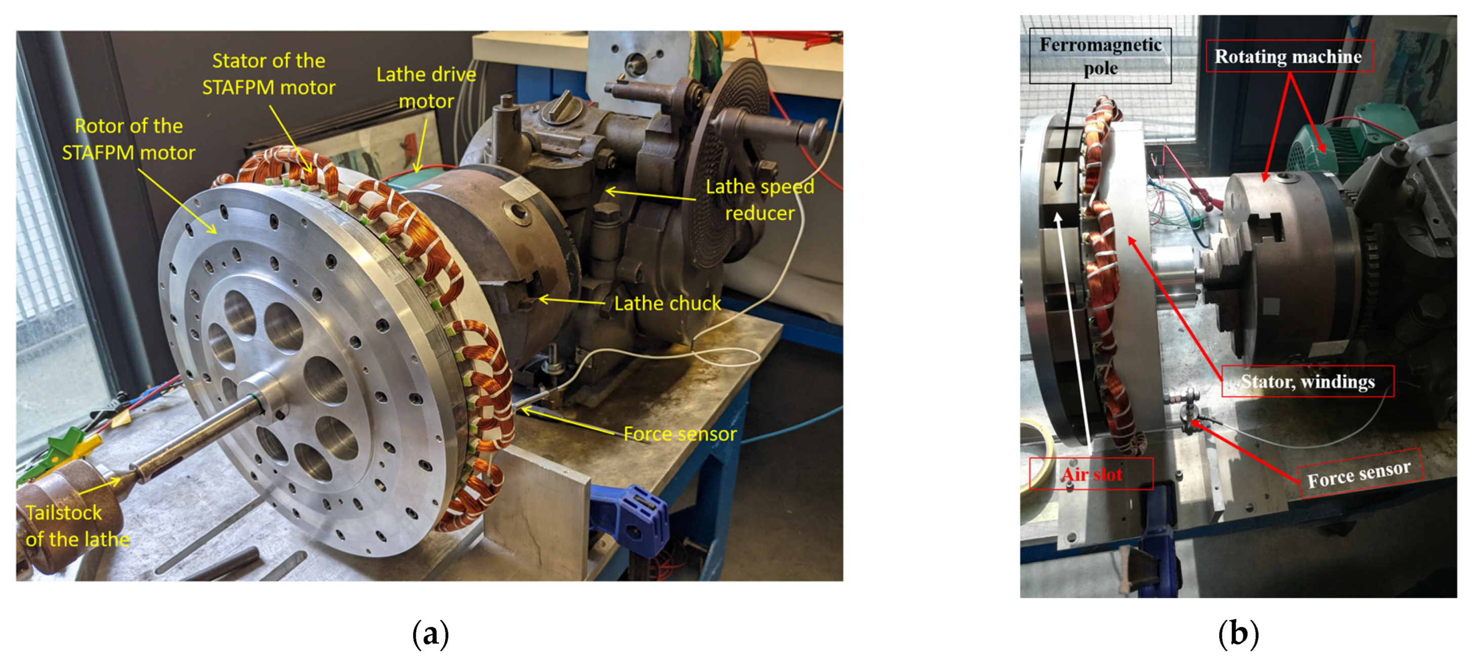
Figure 2a shows the experimental test bench used to measure motor torque as a function of rotor position. The stator was mounted on the bench free to rotate around its bearing. In Figure 2a, the permanent magnets are mounted on the STAFPM motor, while in Figure 2b, the permanent magnets are not mounted.

To measure any tangential force $F_T^S$ applied to the stator, a force sensor is fitted between the stator and the chassis of the test bench, as shown in Figure 2b. The force sensor’s application point is situated close to the stator’s outer edge, which is separated from the rotor axis by the following distance:

$$r_{FS}=134.7 \mathrm{m}\mathrm{m}$$

(30)

On the opposite side the load cell application point, weights were positioned on the outer edge of the stator to achieve equilibrium at standstill, so that the measured force was zero.

The force sensor delivers a voltage $V_F$ proportional to the tangential force $F_T^S$ with a coefficient $c_{FV}$. Two Entran force sensors were used, depending on the torque value to be measured: a 25 N force sensor (ELPS-T1M-25N, Entran Devices, Fairfield, NJ, USA) and a 100 N force sensor (ELPS-T2M-100N, Entran Devices, Fairfield, NJ, USA). The Full-Scale Output (FSO) was 10 V for 25 N and 10 V for 100 N, which provided the $c_{FV}$ coefficients of 2.5 N/V and 10 N/V, respectively. For the two sensors, the combined non-linearity and hysteresis error was 0.5 % of the FSO and the zero drift was 1 % of the FSO. The Entran MSC6 sensor conditioner (Entran Devices, Fairfield, NJ, USA) measures the voltage $V_F$, which is then acquired in function of time by a digital oscilloscope.

Due to the action–reaction principle, the torque applied on the rotor $C_R$ is related to the torque applied on the stator $C_{Stat}$:

$$C_R=-C_{Stat}=-r_{FS}·F_T^S=-r_{FS}·c_{FV}{V}_F$$

(31)

The non-linearity and hysteresis measurement error on the torque with the 25 N sensor was $\pm 0.017 \mathrm{N}\mathrm{m}$ and with the 100 N sensor was $\pm 0.067 \mathrm{N}\mathrm{m}$.

A drive motor located on the test bench set the prototype’s rotor in motion at a relatively low constant speed (0.29 rpm). This speed was set at the very start of the test. A source of DC current provided the stator winding’s phases. By correctly connecting the phases, as indicated in Figure 3, three types of supplies can be easily completed.

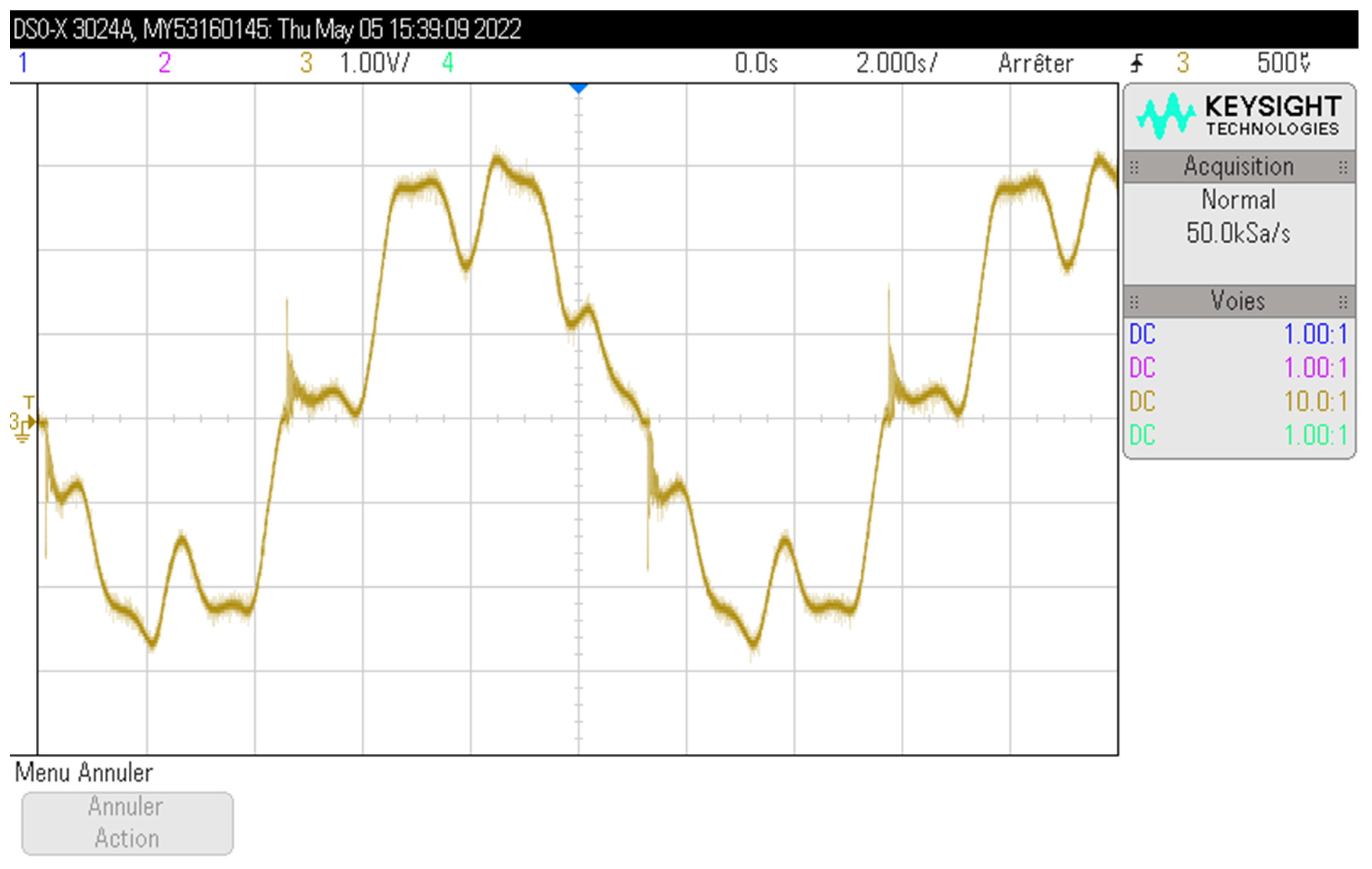
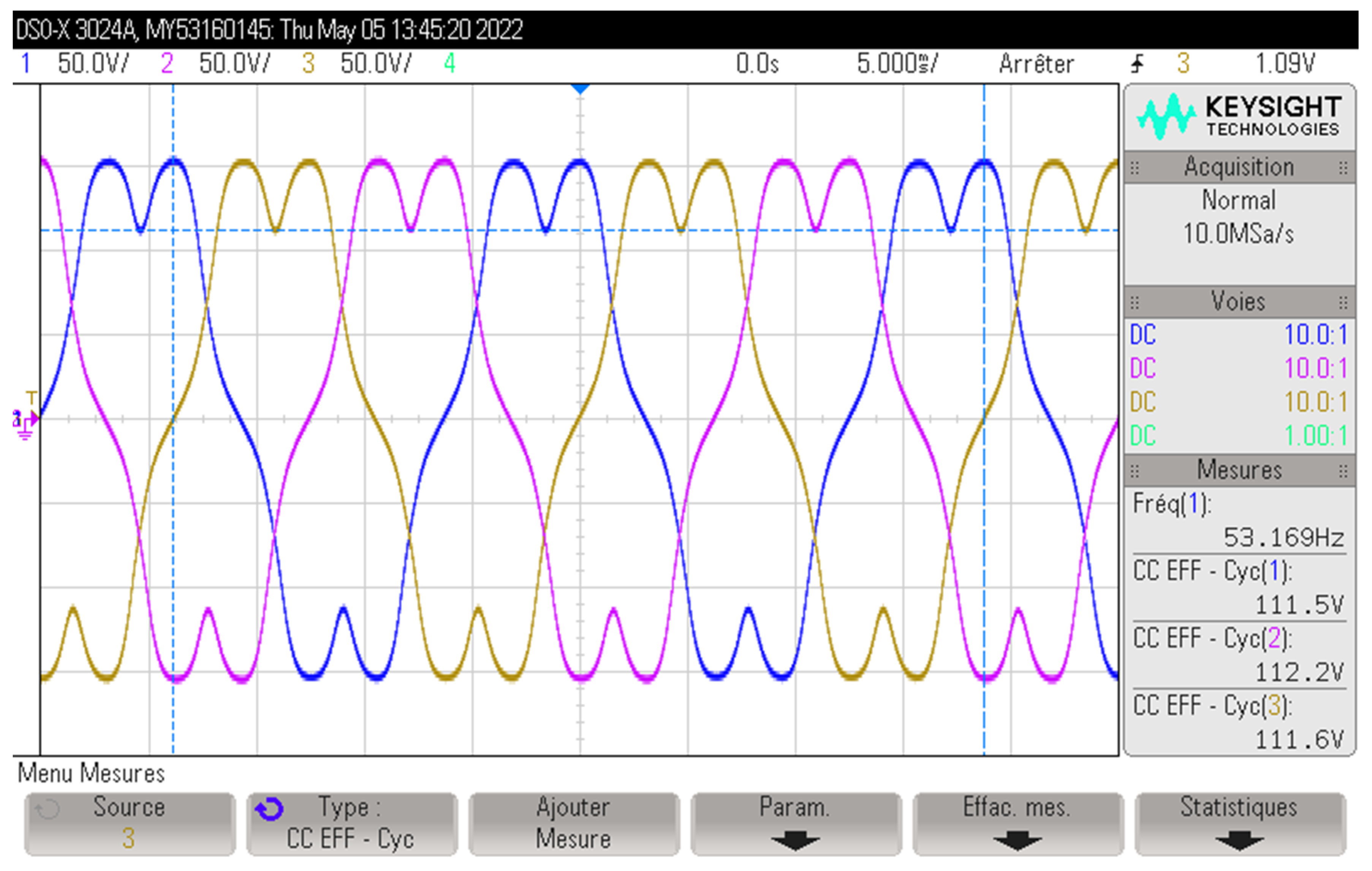
Figure 4 shows an example of the force sensor’s output voltage $V_F$ as a function of time displayed on an oscilloscope, representing the torque applied to the stator. In this example, the permanent magnets are mounted on the rotor, the stator is supplied by the three-phase supply configuration (Figure 3c) with $I_c=0.6 \mathrm{A}$, and the force sensor used is 100 N.

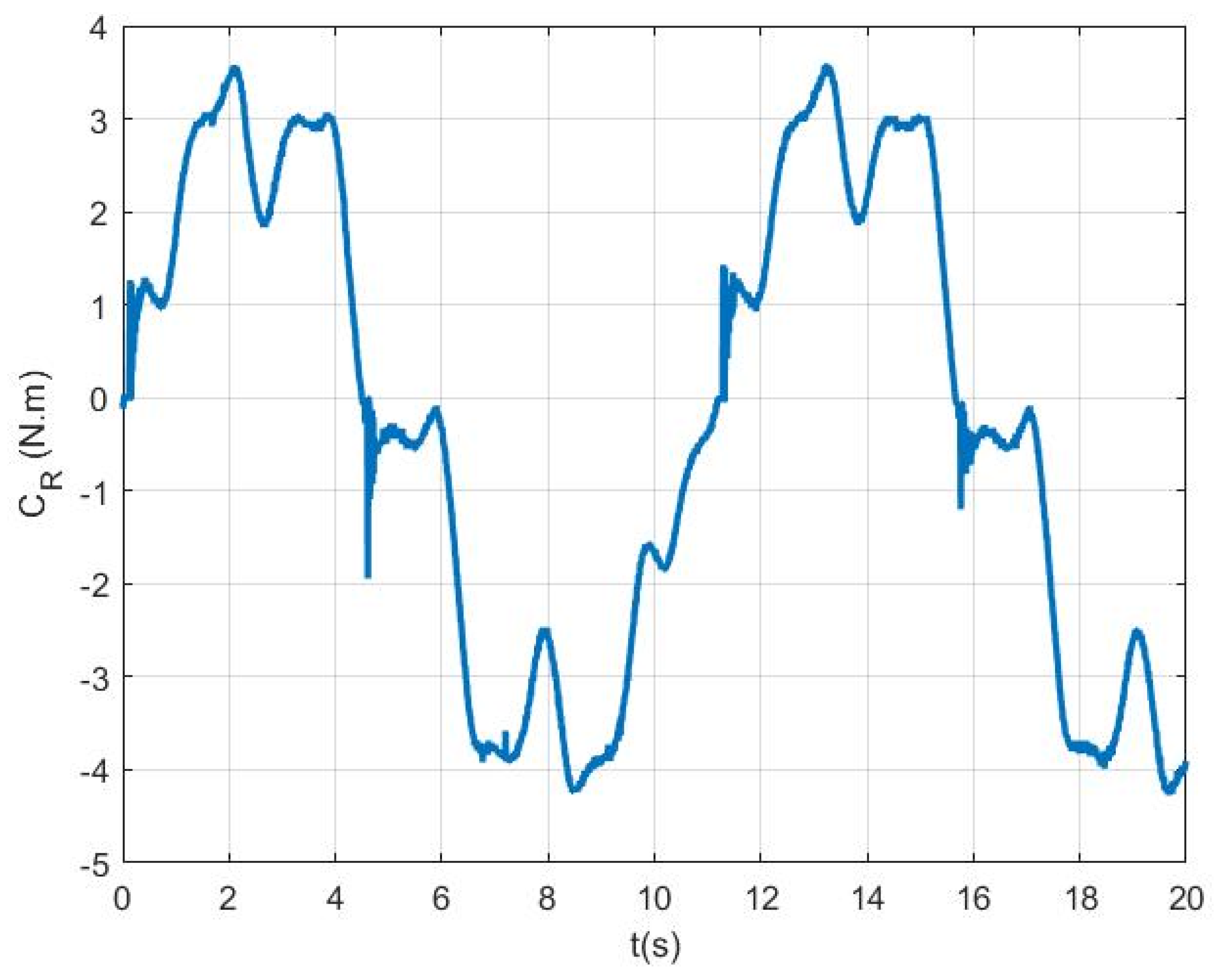
According to (31), Figure 5 shows the torque applied on the rotor $C_R$ corresponding to the output voltage $V_F$ presented in Figure 4.

It can be seen that the delivered signal is not perfect and must be treated numerically, with a dedicated MATLAB (R2016b) program.

The first observation is the detection of parasitic noise in the measured torque, which must be filtered. A moving average filter was used to filter the measured signal.

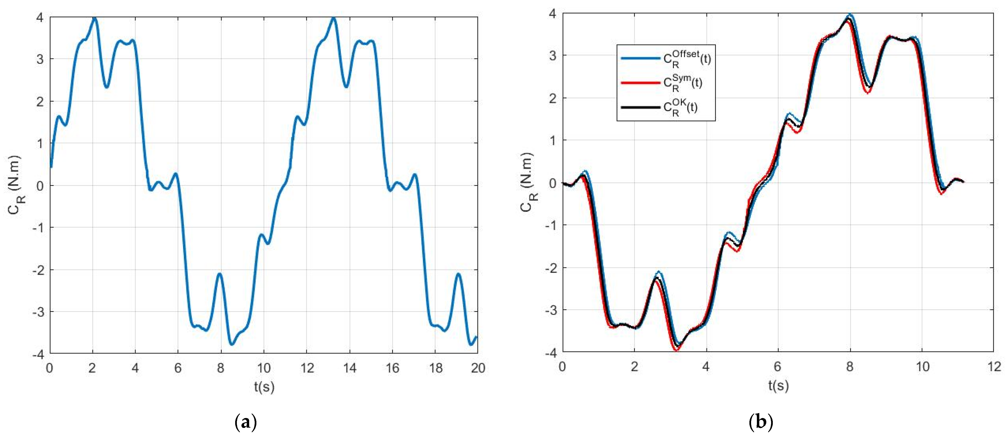
The second observation is that the signal is not symmetric along the vertical axis: the maximal torque value is not opposite its minimal value. It is also not symmetric along the horizontal axis: over a period, the duration of the positive torque is not equal to its negative value. So, an offset was applied to position the horizontal axis at the zero torque level. Figure 6a shows the resulting $C_R^{\mathrm{O}\mathrm{f}\mathrm{f}\mathrm{s}\mathrm{e}\mathrm{t}}\left(t\right)$ torque. To equalize along the vertical and the horizontal axes, we calculated the torque $C_R^{\mathrm{S}\mathrm{y}\mathrm{m}}\left(t\right)$ symmetrical to $C_R^{\mathrm{O}\mathrm{f}\mathrm{f}\mathrm{s}\mathrm{e}\mathrm{t}}\left(t\right)$ with respect to the point $\left({\displaystyle \frac{T}{2}},0\right)$ on the horizontal axis. The final signal $C_R^{\mathrm{O}\mathrm{K}}\left(t\right)$ was the average of the two signals $C_R^{\mathrm{S}\mathrm{y}\mathrm{m}}\left(t\right)$ and $C_R^{\mathrm{O}\mathrm{f}\mathrm{f}\mathrm{s}\mathrm{e}\mathrm{t}}\left(t\right)$. All three signals are shown in Figure 6b.

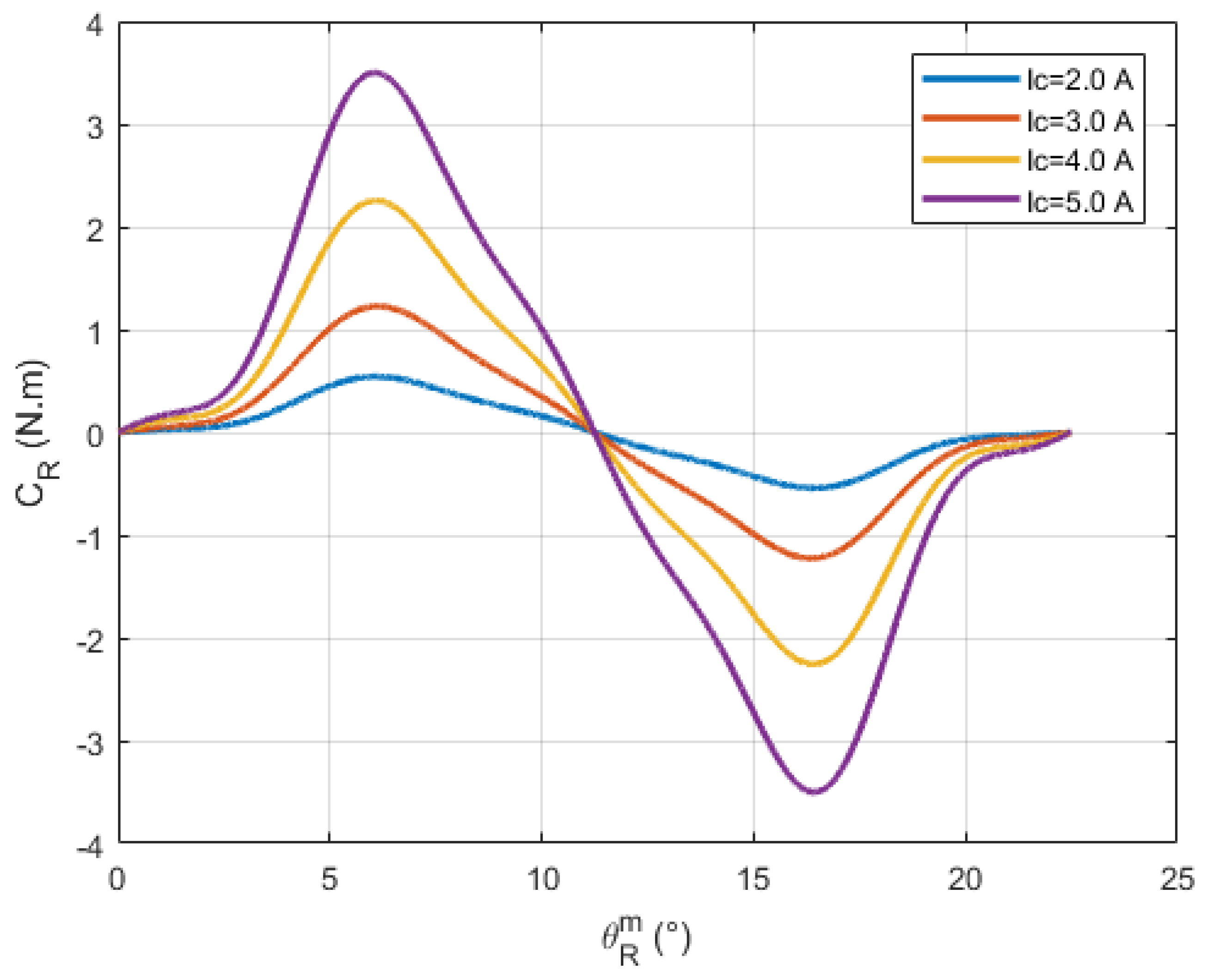
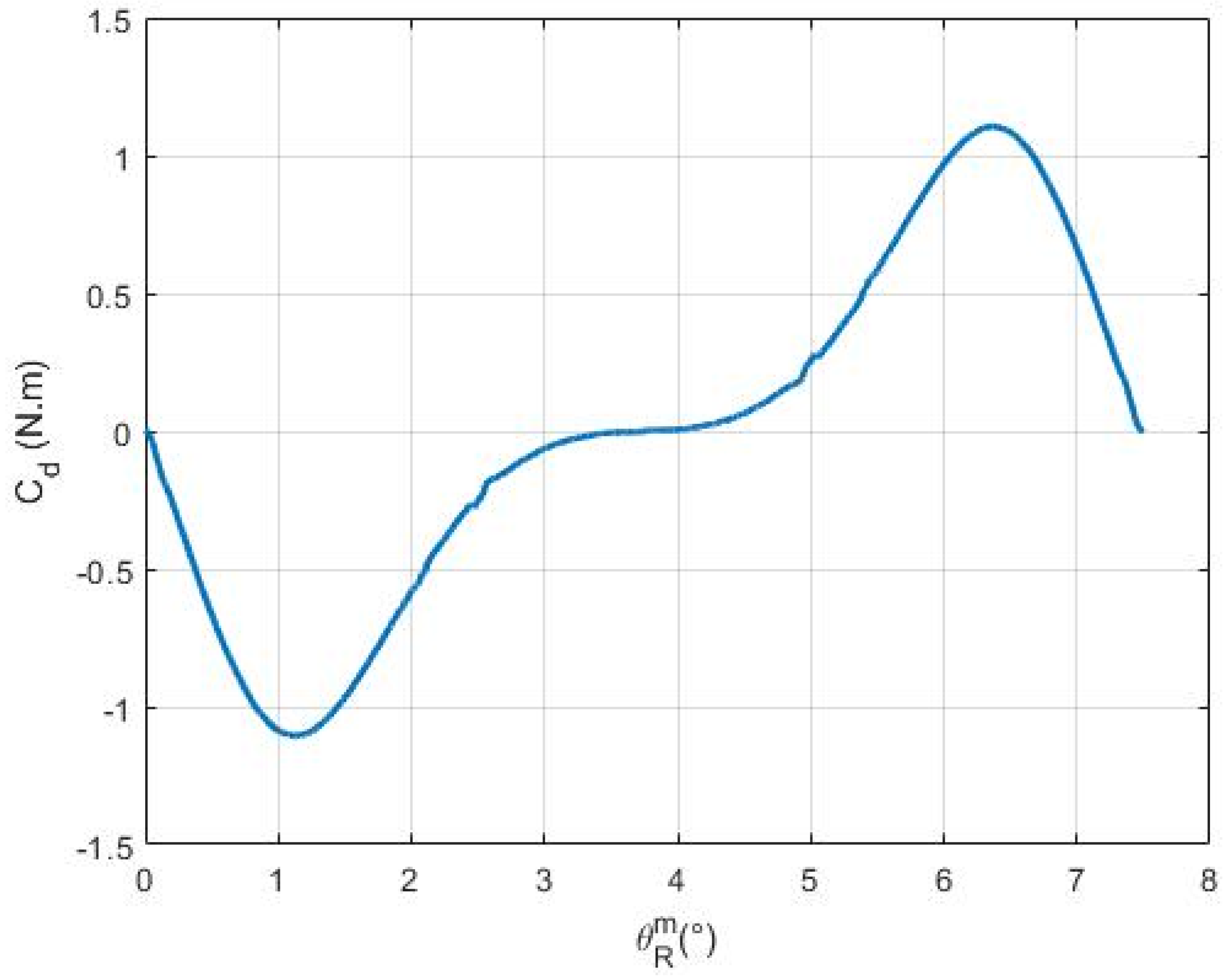
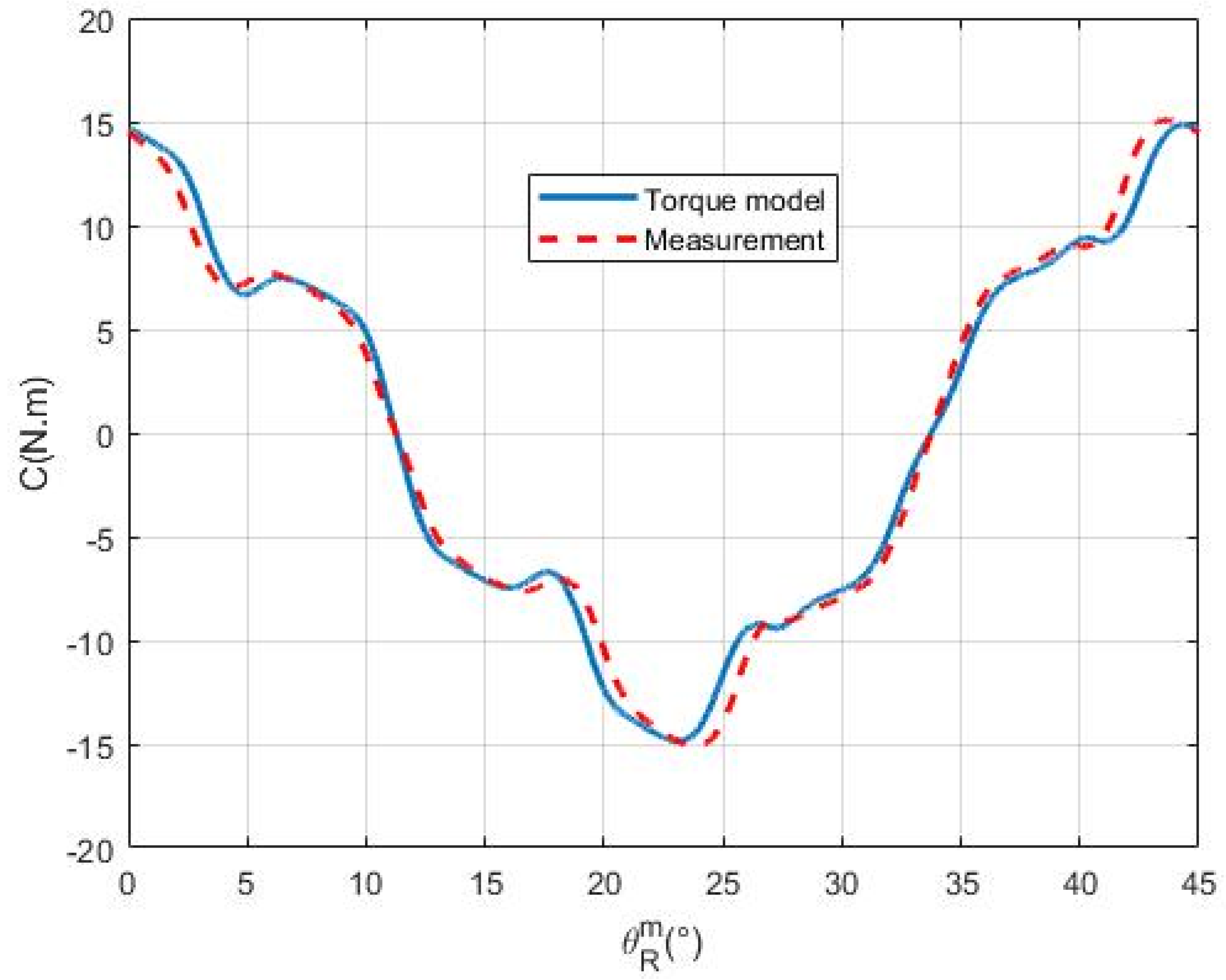
With rotor speed known, the torque can then be plotted as a function of rotor position ${\theta }_R^m$ over a mechanical period in Figure 7.

5. Identification of the Parameters of the Lumped Electromechanical Model

5.1. Static Torque Measurements Without Permanent Magnets

In this section, we assume that the permanent magnets are not fixed to the rotor. If you have a spoke-type structure, keep in mind that the ferromagnetic pole pieces are attached to a non-magnetic rotor yoke, which is not ferromagnetic.

5.1.1. Single-Phase Supply

Phase 1 of the prototype is powered by the single-phase supply configuration, as shown in Figure 3a. The speed of the driven rotor is chosen to be extremely low (0.29 rpm) to avoid frequency-related effects. Figure 8 displays the measured static torque curves obtained for several current values.

The derivatives of the self-inductance with respect to the rotor’s mechanical angular position ${\displaystyle \frac{d{L}_1\left({\theta }_R^m\right)}{d{\theta }_R^m}}$ can be deduced from $C_{R1}\left({\theta }_R^m\right)$ (Figure 8) and using (15) with $k=1$. The shape of these derivatives is displayed in Figure 9 for the different current values chosen previously. Clearly, the current value has no effect on the derivatives of the self-inductance as a function of rotor position. This demonstrates that the magnetic circuit is not saturated when the permanent magnets are not mounted.

From the measurements illustrated in Figure 8, it is possible to break down the torque as a function of rotor position into harmonics. The torque can be expressed as follows, considering the periodicity and the symmetry with respect to the origin.

$$C_{R1}\left({\theta }_R^m\right)=\sum _{n=1}^{nh}{s}_n\mathit{sin}\left(2np{\theta }_R^m\right)$$

(32)

The derivative of the self-inductance of phase $k$ can be expressed in terms of the harmonics $s_n$ of the static torque due to one phase $C_{Rk}$:

$${\displaystyle \frac{d{L}_k\left({\theta }_R^m\right)}{d{\theta }_R^m}}=2{\displaystyle \frac{C_{Rk}\left({\theta }_R^m\right)}{I_c^2}}={\displaystyle \frac{2}{I_c^2}}\sum _{n=1}^{nh}{s}_n\mathit{sin}\left(2n\left(p{\theta }_R^m-\left(k-1\right){\displaystyle \frac{2\pi }{3}}\right)\right)$$

(33)

From (24) and (33), we can identify the harmonic expression of the derivative of the self-inductances:

$${dl}_n={\displaystyle \frac{2}{I_c^2}}{s}_n$$

(34)

The values of the first-five harmonics of the inductance derivative are provided in

Table 2. The first-five harmonics of the self-inductance derivatives.

$\mathit{d}{\mathit{l}}_{\mathit{n}}=$	$\frac{2}{{\mathit{I}}_{\mathit{c}}^2}{\mathit{s}}_1\times {10}^{-2}$	$\frac{2}{{\mathit{I}}_{\mathit{c}}^2}{\mathit{s}}_2\times {10}^{-2}$	$\frac{2}{{\mathit{I}}_{\mathit{c}}^2}{\mathit{s}}_3\times {10}^{-2}$	$\frac{2}{{\mathit{I}}_{\mathit{c}}^2}{\mathit{s}}_4\times {10}^{-2}$	$\frac{2}{{\mathit{I}}_{\mathit{c}}^2}{\mathit{s}}_5\times {10}^{-2}$
$I_c=2A$	20.27	−5.64	−4.41	0.41	1.60
$I_c=3A$	20.38	−5.82	−4.48	0.54	1.41
$I_c=4A$	20.84	−5.96	−4.94	0.54	1.79
$I_c=5A$	20.68	−5.52	−5.01	0.44	1.79

when varying the current in phase 1. As we observed, a little variation in the harmonic values with respect to the current is reflected. The self-inductance’s harmonics, $l_n$, is determined using (25).

5.1.2. Double-Phase Supply

The double-phase supply is considered also with the absence of the permanent magnets, and only phases 2 and 3 are fed with the DC current. Figure 3b shows the phase connections and supplied currents for this configuration. A very-low speed is used to drive the rotor (0.29 rpm). The measured static torque as a function of the mechanical angle ${\theta }_R^m$ is shown in Figure 10 with two distinct current values.

For the current supply configuration under consideration, and based on the electromechanical model, the torque is expressed by (16). Figure 11 illustrates the normalized torque coefficient, given by $2C_{R23}\left({\theta }_R^m\right)/I_c^2$, for the two previously applied current values. The figure demonstrates that the torque characteristics remain invariant with respect to the magnitude of the current, indicating that the torque profile is predominantly governed by the rotor position ${\theta }_R^m$ rather than the current amplitude.

Based on the measurements depicted in Figure 10, the torque as a function of the rotor position can be decomposed into its harmonic components. This decomposition leverages the periodic and symmetric nature of the torque waveform with respect to the origin, allowing for a Fourier series representation that captures the underlying electromechanical behavior:

$$C_{R23}\left({\theta }_R^m\right)=\sum _{n=1}^{nh}{sa}_n\mathit{sin}\left(2np{\theta }_R^m\right)$$

(35)

Table 3. The first-five harmonics of $2C_{R23}\left({\theta }_R^m\right)/I_c^2$.

	$\frac{2}{{\mathit{I}}_{\mathit{c}}^2}{\mathit{s}\mathit{a}}_1\times {10}^{-2}$	$\frac{2}{{\mathit{I}}_{\mathit{c}}^2}{\mathit{s}\mathit{a}}_2\times {10}^{-2}$	$\frac{2}{{\mathit{I}}_{\mathit{c}}^2}{\mathit{s}\mathit{a}}_3\times {10}^{-2}$	$\frac{2}{{\mathit{I}}_{\mathit{c}}^2}{\mathit{s}\mathit{a}}_4\times {10}^{-2}$	$\frac{2}{{\mathit{I}}_{\mathit{c}}^2}{\mathit{s}\mathit{a}}_5\times {10}^{-2}$
$I_c=2A$	−21.23	−9.58	−14.00	−2.32	−1.16
$I_c=3A$	−21.28	−9.33	−14.01	−2.05	−1.04

presents the amplitudes of the first-five harmonics of the normalized torque expression, $2C_{R23}\left({\theta }_R^m\right)/I_c^2$, for the two different current values. The results indicate that the harmonic amplitudes exhibit minimal variation with respect to the supplied current, confirming that the torque harmonic structure is largely independent of current magnitude.

The derivative of the mutual inductance between phases 2 and 3 is given by (17). Then using (17), (33), and (35), the final expression of the mutual inductance of phase $k$ is:

$${\displaystyle \frac{d{M}_k\left({\theta }_R^m\right)}{d{\theta }_R^m}}={\sum }_{n=1}^{nh}{dm}_n\mathit{sin}\left(2n\left(p{\theta }_R^m-\left(k-1\right){\displaystyle \frac{2\pi }{3}}\right)\right),$$

(36)

with ${dm}_n$, the harmonics of the mutual inductance derivative:

$${dm}_n={\displaystyle \frac{1}{I_c^2}}\left(2s_n\mathit{cos}\left(n{\displaystyle \frac{2\pi }{3}}\right)-{sa}_n\right)$$

(37)

The harmonic components $m_n$ of the mutual inductance can be determined using (28). The derivative of the inductance matrix is then evaluated using (38), as it incorporates the derivatives associated with variations in both self- and mutual inductances. These derivatives are expressed in terms of the harmonic components of the single-phase static torque, as defined in (32), and the double-phase static torque, as shown in (35).

$${\displaystyle \frac{d\mathit{L}\left({\theta }_R^m\right)}{d{\theta }_R^m}}=\left[\begin{array}{ccc}{\displaystyle \frac{d{L}_1\left({\theta }_R^m\right)}{d{\theta }_R^m}}& {\displaystyle \frac{d{M}_3\left({\theta }_R^m\right)}{d{\theta }_R^m}}& {\displaystyle \frac{d{M}_2\left({\theta }_R^m\right)}{d{\theta }_R^m}}\\ {\displaystyle \frac{d{M}_3\left({\theta }_R^m\right)}{d{\theta }_R^m}}& {\displaystyle \frac{d{L}_2\left({\theta }_R^m\right)}{d{\theta }_R^m}}& {\displaystyle \frac{d{M}_1\left({\theta }_R^m\right)}{d{\theta }_R^m}}\\ {\displaystyle \frac{d{M}_2\left({\theta }_R^m\right)}{d{\theta }_R^m}}& {\displaystyle \frac{d{M}_1\left({\theta }_R^m\right)}{d{\theta }_R^m}}& {\displaystyle \frac{d{L}_3\left({\theta }_R^m\right)}{d{\theta }_R^m}}\end{array}\right]$$

(38)

5.1.3. Self- and Mutual Inductances Computations

The expressions of self- and mutual inductances are presented by (10) and (12) respectively. Their harmonics $l_n$ and $m_n$ are deduced from the self- and mutual inductance derivatives’ harmonics ${dl}_n$ and ${dm}_n$. The latter are derived from torque measurements carried out for the two power supply configurations presented above.

It remains to identify the mean values $L_s$ and $M_s$ of self- and mutual inductances. According to (26) and (29), further electrical measurements should be carried out at the particular rotor positions ${\theta }_R^L$ and ${\theta }_R^M$. This is performed by estimating $L_1\left({\theta }_R^L\right)$ at ${\theta }_R^L$ and the mutual inductance $M_k\left({\theta }_R^M\right)$ at ${\theta }_R^M$.

When the permanent magnets are removed, these electrical measurements are made at blocked rotor positions rather than on the torque test bench. ${\theta }_R^L$ and ${\theta }_R^M$ are chosen among the rotor’s equilibrium positions. After testing several equilibrium positions for these electrical measurements, the initial position ${\theta }_R^m=0$ was finally selected to perform the measurements:

$${\theta }_R^L={\theta }_R^M=0$$

(39)

When phase 1 is energized, the original position is unstable, although it is an equilibrium position. Thus, the rotor is blocked while the measurement is being taken. A sinusoidal current with an RMS value of 1 A and a frequency of 50 Hz is applied to phase 1 only. There is no supply for the other phases. Every phase’s voltage is measured in addition to the active and reactive powers. This procedure is repeated for phases 2 and 3 under identical situations.

Table 4. Main electrical parameters.

Electrical Parameter	Phase 1 Supplied	Phase 2 Supplied	Phase 3 Supplied
$\mathrm{Resistance}, R_s (\Omega )$	13.10	13.30	12.90
$\mathrm{Self-inductance}, L_s \left(\mathrm{m}\mathrm{H}\right)$	38.20	37.90	37.90
$\mathrm{Mutual} \mathrm{inductance}, M_x \left(\mathrm{m}\mathrm{H}\right)$	−6.20	−6.00	−9.60
$\mathrm{Mutual} \mathrm{inductance}, M_y \left(\mathrm{m}\mathrm{H}\right)$	−9.90	−10.00	−10.00

provides a summary of the extracted parameters from these measurements.

From the electrical measurements, the values of self- and mutual inductances for the unstable equilibrium position are deduced:

$$\left\{\begin{array}{c}{L}_1\left(0\right)=38.0 \mathrm{mH}\\ L_{12}\left(0\right)=M_3\left(0\right)=-6.1 \mathrm{mH}\end{array}\right.$$

(40)

Eventually, the mean values of self- and mutual inductances are given by:

$$\left\{\begin{array}{c}{L_S=L}_1\left(0\right)-{\displaystyle \sum _{n=1}^{\infty }}{l}_n\\ { M}_S=M_3\left(0\right)-{\displaystyle \sum _{n=1}^{\infty }}{m}_{n}cos\left(2n{\displaystyle \frac{4\pi }{3}}\right)\end{array}\right.$$

(41)

Figure 12 shows self- and mutual inductances obtained from (10) and (12).

5.1.4. Conclusion of the Tests Without Permanent Magnets

The tests were conducted with the rotor demagnetized, i.e., without the permanent magnets. Static torque as a function of rotor position was measured under both single-phase and two-phase supply configurations. These measurements enabled the determination of the self- and mutual inductances, along with the harmonic components of their derivatives. Based on the rotor position and the phase currents, torque saliency can then be evaluated using the derived parameters from the torque model.

5.2. Static Torque Measurements with Permanent Magnets

5.2.1. Cogging Torque

Cogging torque refers to the torque measured when the permanent magnets are mounted on the rotor and when the stator is de-energized. The measured cogging torque is shown in Figure 13.

The cogging torque’s period in mechanical degrees is equal to ${\displaystyle \frac{360}{n_e}}=7.5°$, which corresponds to one tooth pitch. As a result, the cogging torque as a function of the rotor’s angular position can be expressed by:

$$C_d\left({\theta }_R^m\right)={\sum }_{n=1}^{nh}{sd}_n\mathit{sin}\left(n{n}_e{\theta }_R^m\right),$$

(42)

where ${sd}_n$ is the cogging torque harmonics of rank $n$, $n_e$ is the number of slots. Thus, from the data in Figure 13, the values of the first-five harmonics ${sd}_n$ of $C_d\left({\theta }_R^m\right)$ are calculated and presented in

Table 5. The first-five harmonics of $C_d\left({\theta }_R^m\right)$.

${\mathit{s}\mathit{d}}_1$	${\mathit{s}\mathit{d}}_2$	${\mathit{s}\mathit{d}}_3$	${\mathit{s}\mathit{d}}_4$	${\mathit{s}\mathit{d}}_5$
−0.7418	−0.4526	−0.0527	0.0176	0.0135

.

5.2.2. Derivative of the No-Load Flux

In this test configuration, the rotor retains its permanent magnets. The motor operates under open-circuit conditions (i.e., no current is supplied), while an external motor drives the rotor at a constant speed of 400 rpm. Under these no-load conditions, the back electromotive force (e.m.f.) at the terminals of each phase is measured. As illustrated in Figure 14, the e.m.f. exhibits a peak amplitude of $V_{peak}=152 \mathrm{V}$.

The derivatives of the no-load fluxes with respect to the rotor position ${\theta }_R^m$ can be obtained from (20). As shown in Figure 15, the flux derivative’s period in mechanical degrees is equal to ${\displaystyle \frac{360}{p}}=45°$, which corresponds to one pair of poles.

Equation (22) provides the expression of the derivatives of the no-load flux as a function of rotor position in terms of its harmonics. Utilizing the data presented in Figure 15, the values of the first eleven harmonics, ${df}_n$ of ${\displaystyle \frac{{d\varphi }_{vk}}{{d\theta }_R^m}}\left({\theta }_R^m\right)$, are computed and summarized in

Table 6. The first-eleven harmonics of ${\displaystyle \frac{{d\varphi }_{vk}}{{d\theta }_R^m}}\left({\theta }_R^m\right)$.

${\mathit{d}\mathit{f}}_1$	${\mathit{d}\mathit{f}}_2$	${\mathit{d}\mathit{f}}_3$	${\mathit{d}\mathit{f}}_4$	${\mathit{d}\mathit{f}}_5$	${\mathit{d}\mathit{f}}_6$
−3.7012	−0.0031	−0.1698	−0.0023	−0.5455	0.0
${df}_7$	${df}_8$	${df}_9$	${df}_{10}$	${df}_{11}$
−0.0155	0.0	0.0025	0.0	−0.0452

. The selection of eleven harmonics corresponds to the spatial periodicity of the stator slots, which is 7.5°, relative to the 45° periodicity of the no-load flux waveform.

5.2.3. No-Load Flux Computation

The no-load flux derivatives’ harmonics, ${df}_n$ (Table 6), were found using e.m.f. measurements. The no-load flux’s harmonics of ${\varphi }_{vk}\left({\theta }_R^m\right)$, $f_n$ are provided using knowledge of ${df}_n$ (23).

Table 7. The first-five harmonics of ${\varphi }_{vk}\left({\theta }_R^m\right)$.

${\mathit{f}}_1$	${\mathit{f}}_2$	${\mathit{f}}_3$	${\mathit{f}}_4$	${\mathit{f}}_5$
0.4625	0.0	0.071	0.0	−0.0136

shows the values of the first-five harmonics $f_n$ of ${\varphi }_{vk}\left({\theta }_R^m\right)$.

Using its harmonics, the no-load fluxes ${\varphi }_{vk}\left({\theta }_R^m\right)$ using (8) are displayed in Figure 16.

5.2.4. Conclusion of the Tests with Permanent Magnets

Experiments were carried out with the rotor’s permanent magnets attached and with zero current supplied to the stator windings. The harmonic components of the no-load flux and the cogging torque were determined under these circumstances. These harmonics serve as key parameters to compute the cogging torque and electromagnetic torque as functions of rotor position and phase currents. With all the parameters of the torque model now established, the validation of the model takes up in the following section.

6. Validation of the Torque Presented by the Lumped Parameter Model

6.1. Static Torque Measurement Without Permanent Magnets and Three-Phase Supply

The permanent magnets were not yet mounted on the rotor. There were only the ferromagnetic pole pieces. The stator was supplied with a constant DC current $I_C=2 \mathrm{A}$. Figure 3c shows the configuration used when all three phases were supplied with a constant current. The torque was measured on the test bench and compared to the one calculated from the saliency torque model. The expression of the saliency torque is presented by (43).

$$C_R\left({\theta }_R^m\right)={\displaystyle \frac{1}{2}}\left\{\begin{array}{ccc}{I}_C& -{\displaystyle \frac{I_C}{2}}& -{\displaystyle \frac{I_C}{2}}\end{array}\right\}·{\displaystyle \frac{d\mathit{L}\left({\theta }_R^m\right)}{d{\theta }_R^m}}·\left\{\begin{array}{c}{I}_C\\ -{\displaystyle \frac{1}{2}}{I}_C\\ -{\displaystyle \frac{1}{2}}{I}_C\end{array}\right\}$$

(43)

Equation (38) presents the derivative of the inductance matrix. The harmonics of the derivatives of the self- and mutual inductances can be found in Table 2 and Table 3 with the same current value of the above mentioned test, i.e., $2 \mathrm{A}$.

The torque calculated using the saliency-based model and the actual torque are contrasted in Figure 17. The accuracy of the determined parameters and the precision of the numerical modeling approach were validated by the strong agreement between the experimental results and the model estimates. This association demonstrates how well the torque model captured the key aspects of the machine’s electromagnetic behavior.

6.2. Static Torque Measurement with Permanent Magnets

6.2.1. Single-Phase Supply

The rotor contains permanent magnets. Only phase 1 was supplied with a DC current, as shown in Figure 3a. Torque was measured on the test bench and compared with that calculated from the torque model. The aim was to verify the model and the estimated parameters, enabling the calculation of salience, electromagnetic, and cogging torque. For this single-phase test, the torque model presented in (6) can be written by expanding the matrix product:

$$C_R\left({\theta }_R^m\right)=C_d\left({\theta }_R^m\right)+I_C{\displaystyle \frac{d{\mathsf{\varphi }}_{v1}}{d{\theta }_R^m}}\left({\theta }_R^m\right)+{\displaystyle \frac{1}{2}}{\displaystyle \frac{d{L}_1\left({\theta }_R^m\right)}{d{\theta }_R^m}}{I}_c^2$$

(44)

For $I_C=1 \mathrm{A}$, the measured and calculated torques are presented in Figure 18a. Despite the relatively large ripples in the static torque at a low current, the torque model could accurately replicate them.

The measured and computed torques for $I_C=3.6 \mathrm{A}$ are shown in Figure 18b. At higher current levels, it is evident that the static torque shows less ripple. The calculated torque stayed within an acceptable margin of accuracy, even though the difference between the torque determined by the model and the actual observations marginally increased under these circumstances. This indicates that, in spite of the small errors, the torque model remains valid even at high excitation levels.

6.2.2. Double-Phase Supply

The rotor kept its permanent magnets in this test setup. Figure 3b shows that a direct current is used to supply phases 2 and 3. Using the established torque model, the resulting torque under double-phase excitation was calculated (45) and compared to the test bench experimental observations. The torque characteristics for the double-phase supply condition are provided by this comparison, which also serves to confirm the identified model parameters.

$$C_R\left({\theta }_R^m\right)=C_d\left({\theta }_R^m\right)+I_C\left({\displaystyle \frac{d{\mathsf{\varphi }}_{v2}}{d{\theta }_R^m}}\left({\theta }_R^m\right)-{\displaystyle \frac{d{\mathsf{\varphi }}_{v3}}{d{\theta }_R^m}}\left({\theta }_R^m\right)\right)+{\displaystyle \frac{1}{2}}\left({\displaystyle \frac{d{L}_2\left({\theta }_R^m\right)}{d{\theta }_R^m}}+{\displaystyle \frac{d{L}_3\left({\theta }_R^m\right)}{d{\theta }_R^m}}-2{\displaystyle \frac{d{M}_1\left({\theta }_R^m\right)}{d{\theta }_R^m}}\right)I_c^2$$

(45)

For $I_C=2.0 \mathrm{A}$, the measured and calculated torques are presented in Figure 19. It can be seen that the torque model produces results that remain acceptable in relation to the measured results.

6.2.3. Three-Phase Supply

The rotor is still fitted with permanent magnets in this test situation. The three-phase direct current setup shown in Figure 3c was used to supply power to the motor. To verify the determined parameters, torque values were calculated using the previously developed torque model and contrasted with the experimental findings from the test bench. The torque formulation for the three-phase supply was kept in its matrix form due to the complexity of the expressions involved, as it would take too long to fully develop analytically.

$$C_R\left({\theta }_R^m\right)=C_d\left({\theta }_R^m\right)+\left\{\begin{array}{ccc}{I}_C& -{\displaystyle \frac{I_C}{2}}& -{\displaystyle \frac{I_C}{2}}\end{array}\right\}\left\{\begin{array}{c}{\displaystyle \frac{d{\mathsf{\varphi }}_{v1}}{d{\theta }_R^m}}\left({\theta }_R^m\right)\\ {\displaystyle \frac{d{\mathsf{\varphi }}_{v2}}{d{\theta }_R^m}}\left({\theta }_R^m\right)\\ {\displaystyle \frac{d{\mathsf{\varphi }}_{v3}}{d{\theta }_R^m}}\left({\theta }_R^m\right)\end{array}\right\}+{\displaystyle \frac{1}{2}}\left\{\begin{array}{ccc}{I}_C& -{\displaystyle \frac{I_C}{2}}& -{\displaystyle \frac{I_C}{2}}\end{array}\right\}{\displaystyle \frac{d\mathit{L}\left({\theta }_R^m\right)}{d{\theta }_R^m}}\left\{\begin{array}{c}{I}_C\\ -{\displaystyle \frac{I_C}{2}}\\ -{\displaystyle \frac{I_C}{2}}\end{array}\right\}$$

(46)

For $I_C=2.6 \mathrm{A}$, the measured and the calculated torque values are presented in Figure 20.

This type of current supply, at the specified current level, can be considered equivalent to a particular operating point of a balanced three-phase sinusoidal supply with a corresponding RMS current value, $I_{rms}=1.84 \mathrm{A}$, which is higher than the rated value of $I_{rms}=1.5 \mathrm{A}$ (current density of nearly $5 \mathrm{A}/{\mathrm{m}\mathrm{m}}^2$ in the conductors).

6.3. Summary of the Method

To determine the electromechanical lumped parameter model of the STAFPM motor, we used a static torque bench. The motor torque $C_{mot}\left({\theta }_R^m\right)$, as indicated in Equation (6), is the sum of the cogging torque $C_d\left({\theta }_R^m\right)$, the saliency torque $C_{sail}\left({\theta }_R^m\right)$, and the electromagnetic torque $C_{em}\left({\theta }_R^m\right)$. The saliency torque $C_{sail}\left({\theta }_R^m\right)$ depends on the derivative matrix inductance ${\displaystyle \frac{d\mathit{L}\left({\theta }_R^m\right)}{d{\theta }_R^m}}$, and the electromagnetic torque $C_{em}\left({\theta }_R^m\right)$ depends on the derivative of the no-load flux ${\displaystyle \frac{{d\mathsf{\Phi }}_{\mathit{v}}\left({\theta }_R^m\right)}{d{\theta }_R^m}}$ (see Section 3.3).

To identify the model parameters, we need to proceed in two steps. The first step is to measure the static torque of the motor without the magnets with the static torque bench, in order to obtain the derivative matrix inductance ${\displaystyle \frac{d\mathit{L}\left({\theta }_R^m\right)}{d{\theta }_R^m}}$ and therefore the saliency torque $C_{sail}\left({\theta }_R^m\right)$. The second step is to mount the magnets to the rotor and determine the cogging torque $C_d\left({\theta }_R^m\right)$ with the static torque bench. Finally, with a no-load test, where the motor is driven in rotation, we can deduce the derivative of the no-load flux of the magnets ${\displaystyle \frac{{d\mathsf{\Phi }}_{\mathit{v}}\left({\theta }_R^m\right)}{d{\theta }_R^m}}$ and therefore the electromagnetic torque $C_{em}\left({\theta }_R^m\right)$ by measuring the e.m.f.

One limitation of this method is that it must be performed in this order. Once the magnets are mounted on the rotor, it is almost impossible to go back and perform the tests without the magnets. This method applies to any machine with saliency. It is not useful to proceed in this way with a machine with smooth poles. An alternative to this method is to perform FEA analysis in 2D or 3D for the STAFPM motor, which has a 3D design. Other analysis methods are used with FEA and the Frozen Permeability Method (FPM) [21], and with a Maxwell Stress Tensor and FPM [22].

In future work, the motor can be studied dynamically: supplied via a three-phase inverter and loaded by a hysteresis brake with a dynamic measurement of motor torque. Motor control can be based on the DQ model presented in the next section.

7. Study of the STAFPM Motor Supplied by a Three-Phase Sinusoidal Current System

The behavior of the STAFPM motor was studied using the flux and torque models presented previously, as well as the DQ0 model.

7.1. DQ0 Model

Park transformation was applied to the no-load flux calculated by the flux model, and is shown in Figure 16. Figure 21 shows the DQ0 components $\left\{{\mathsf{\varphi }}_{vD},{\mathsf{\varphi }}_{vQ},{\mathsf{\varphi }}_{v0}\right\}$ of the no-load flux as a function of rotor position.

It can be seen that the quadrature and homopolar components of the no-load flux have zero mean values, which is consistent. The no-load flux’s direct component has the following mean value:

$${\left({\mathsf{\varphi }}_{vD}\right)}_{mean}=0.57 \mathrm{W}\mathrm{b}$$

(47)

The direct-axis and quadrature-axis inductances are now calculated. The generic equation for the magnetic flux, provided by (8), simplifies in the absence of permanent magnets placed between the rotor’s ferromagnetic pole components. In this scenario, the rotor’s saliency effects and stator currents are the only sources of the flux contributions:

$$\mathsf{\Phi }\left({\theta }_R^m\right)=\mathit{L}{(\theta }_R^m)\mathit{I}$$

(48)

For a self-driven synchronous motor, the current $I_k$ of phase $k$ is:

$$I_k=I_{m}cos\left(p{\theta }_R^m+\alpha -\left(k-1\right){\displaystyle \frac{2\pi }{3}}\right)$$

(49)

where $I_m$ is the current magnitude deduced from the rated RMS current ($I_{rms}=1.5 \mathrm{A})$ and $\alpha$ is the phase shift from the rotor position.

For different angles values,$\alpha$, the magnetic fluxes without permanent magnets can be calculated as a function of rotor position. The Park transformation can then be applied to determine the DQ0 components of the fluxes and currents. According to the rotor position, the direct inductance $L_D\left({\theta }_R^m\right)$ and the quadrature inductance $L_Q\left({\theta }_R^m\right)$ are computed for each phase shift as follows.

$$\left\{\begin{array}{c}{L}_D\left({\theta }_R^m\right)={\displaystyle \frac{{\mathsf{\varphi }}_D\left({\theta }_R^m\right)}{I_D\left({\theta }_R^m\right)}}\\ L_Q\left({\theta }_R^m\right)={\displaystyle \frac{{\mathsf{\varphi }}_Q\left({\theta }_R^m\right)}{I_Q\left({\theta }_R^m\right)}}\end{array}\right.$$

(50)

The direct inductance $L_D\left({\theta }_R^m\right)$ and quadrature inductance $L_Q\left({\theta }_R^m\right)$ are shown in Figure 22a and Figure 22b for $\alpha$ angles of $30°$ and $120°$, respectively.

These figures show that the direct and quadrature inductances exhibit ripples that depend on the phase shift, $\alpha$. However, the mean values of these inductances do not depend on the phase shift. The mean values are equal to:

$$\left\{\begin{array}{c}{\left(L_D\right)}_{mean}=48.9 \mathrm{mH} \\ {\left(L_Q\right)}_{mean}=61.5 \mathrm{mH}\end{array}\right.$$

(51)

7.2. Optimal Torque per Ampere by the DQ0 Model

In this section, the direct and quadrature inductances’ ripples and no-load direct flux ripples are neglected. Here are the parameters of the DQ0 model, which are used in the following way.

$$\left\{\begin{array}{c}{\mathsf{\varphi }}_{vD}=0.57 \mathrm{Wb}\\ L_D=48.9 \mathrm{mH} \\ L_Q=61.5 \mathrm{mH}\end{array}\right.$$

(52)

The torque presented by the DQ0 model is:

$$C_{mot}=p{\Phi }_{vD}{i}_Q+p\left(L_D-L_Q\right)i_D{i}_Q$$

(53)

The Maximum Torque Per Ampere (MTPA) algorithm is a relatively efficient control strategy that is currently employed for motors with interior permanent magnets or salient poles [23,24]. This algorithm uses the phase shift α as a variable and maximizes torque for a given stator current value (49).

Thus, the maximum torque obtained at a rated current is:

$$C_{opt}=p{\Phi }_{vD}{I}_Q^{opt}+p\left(L_D-L_Q\right)I_D^{opt}{I}_Q^{opt}=11.87 \mathrm{N}·\mathrm{m},$$

(54)

where $I_D^{opt}$ and $I_Q^{opt}$ are the DQ components of the optimal current:

$$\left\{\begin{array}{c}{I}_D^{opt}=I_{norm}\cos \left({\alpha }_{opt}\right)={\displaystyle \frac{1}{4}}\left(I_b-\sqrt{I_b^2+8I_{norm}^2}\right)\\ I_Q^{opt}=I_{norm}\sin \left({\alpha }_{opt}\right)=\sqrt{I_{norm}^2-{\left(I_D^{opt}\right)}^2} \end{array}\right.,$$

(55)

and ${\alpha }_{opt}$ is the optimal phase shift:

$${\alpha }_{opt}=atan2\left(I_Q^{opt},I_D^{opt}\right)=93.3°$$

(56)

The current $I_b$ is defined as follows:

$$I_b={\displaystyle \frac{{\mathsf{\varphi }}_{vD}}{L_Q-L_D}}=45.24 \mathrm{A}$$

(57)

The norm of the rated current in the DQ0 model is defined as:

$$I_{norm}=\sqrt{I_D^2+I_Q^2}=\sqrt{3}{I}_{rms}=2.6 \mathrm{A}$$

(58)

The torque for the rated current, determined by Equation (54), is displayed in Figure 23 as a function of the phase shift, $\alpha$. It is compared with the electromagnetic torque presented by:

$$C_{em}=p{\Phi }_{vD}{i}_Q$$

(59)

As expected, the optimal torque and electromagnetic torque are obtained, respectively, for $\alpha ={\alpha }_{opt}=93.3°$ and $\alpha =90°$.

7.3. Optimal Torque per Ampere by the Lumped Parameter Model

In this section, the lumped parameter model is used to calculate the torque for the rated current as a function of the rotor position with the phase shift $\alpha$ as a parameter. The currents are presented by (49) and the torque is computed using:

$$\begin{gathered} C_R\left({\theta }_R^m\right)=C_d\left({\theta }_R^m\right)+\left\{\begin{array}{ccc}{I}_1\left({\theta }_R^m\right)& I_2\left({\theta }_R^m\right)& I_3\left({\theta }_R^m\right)\end{array}\right\}\left\{\begin{array}{c}{\displaystyle \frac{d{\mathsf{\varphi }}_{v1}}{d{\theta }_R^m}}\left({\theta }_R^m\right)\\ {\displaystyle \frac{d{\mathsf{\varphi }}_{v2}}{d{\theta }_R^m}}\left({\theta }_R^m\right)\\ {\displaystyle \frac{d{\mathsf{\varphi }}_{v3}}{d{\theta }_R^m}}\left({\theta }_R^m\right)\end{array}\right\} \\ +{\displaystyle \frac{1}{2}}\left\{\begin{array}{ccc}{I}_1\left({\theta }_R^m\right)& I_2\left({\theta }_R^m\right)& I_3\left({\theta }_R^m\right)\end{array}\right\}{\displaystyle \frac{d\mathit{L}\left({\theta }_R^m\right)}{d{\theta }_R^m}}\left\{\begin{array}{c}{I}_1\left({\theta }_R^m\right)\\ I_2\left({\theta }_R^m\right)\\ I_3\left({\theta }_R^m\right)\end{array}\right\} \end{gathered}$$

(60)

Figure 24 shows the torque as a function of rotor position for the optimal phase shift.

It can be noticed from Figure 24 that the torque ripples with a periodicity corresponding to the number of slots, $n_e$. In

Table 8. Comparison of the mean torque from the lumped parameter model and the DQ model.

$\mathit{\alpha }$ Value	Lumped Parameter Model	dq Model
$\alpha =87°$	${\left(C_R({\theta }_R^m)\right)}_{mean}=11.78 \mathrm{N}·\mathrm{m}$	$C_{mot}=11.79 \mathrm{N}·\mathrm{m}$
$\alpha ={\alpha }_{opt}$	${\left(C_R({\theta }_R^m)\right)}_{mean}=11.85 \mathrm{N}·\mathrm{m}$	$C_{mot}=11.87 \mathrm{N}·\mathrm{m}$
$\alpha =100.0°$	${\left(C_R({\theta }_R^m)\right)}_{mean}=11.77 \mathrm{N}·\mathrm{m}$	$C_{mot}=11.78 \mathrm{N}·\mathrm{m}$

, the average torque from the lumped parameter model (60) and the torque from the DQ model (53) are calculated for three different values of phase shift.

Comparing the DQ model to the lumped parameter model, Table 8 demonstrates that the former produces accurate results. Therefore, having a model that effectively computes the DQ model parameters (${\mathsf{\varphi }}_{vD}$, $L_D$ and $L_Q$) is sufficient to size the STAFPM motor.

There are two suggested methods to assess torque ripples. Three-dimensional FEA is an option if the motor has not yet been constructed, but it requires time for analysis design and simulation computations. If the motor is produced, the suggested experimental investigations demonstrate how to determine each parameter of the general electromechanical lumped model. Once these parameters are known, thanks to the static torque measurements performed on the test bench, this model can be used to quickly determine the torque with its ripples.

8. Conclusions

The experimental methodology used in this article uses a dedicated test bench to measure the static torque of an electric motor as a function of rotor position. A novel identification approach is proposed to extract most of the parameters for the electromechanical lumped parameter model of the motor directly from static torque measurements, which are conducted under single-phase, double-phase, and three-phase DC excitations. The experimental data allow for the validation of the proposed identification technique and the identified model parameters, as well as the signal processing algorithms used to mitigate measurement artifacts.

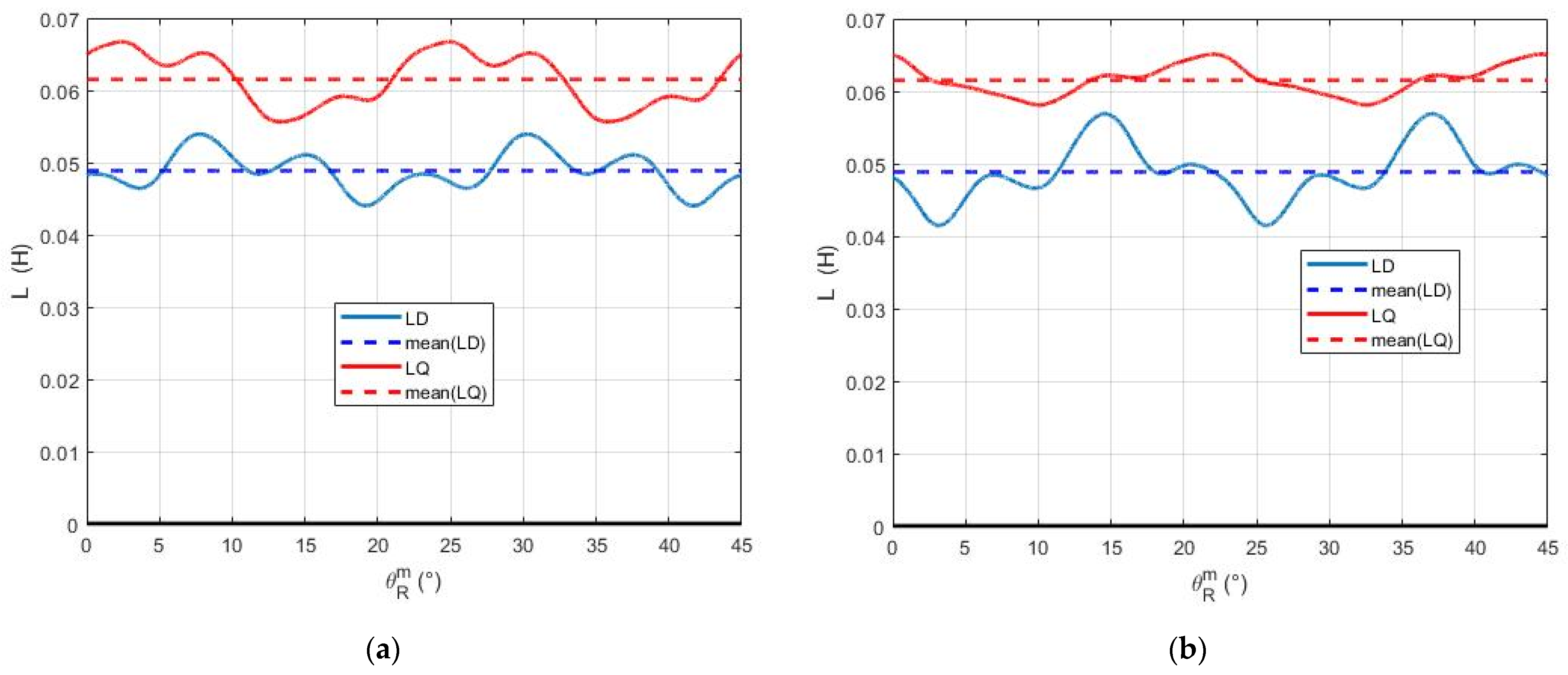
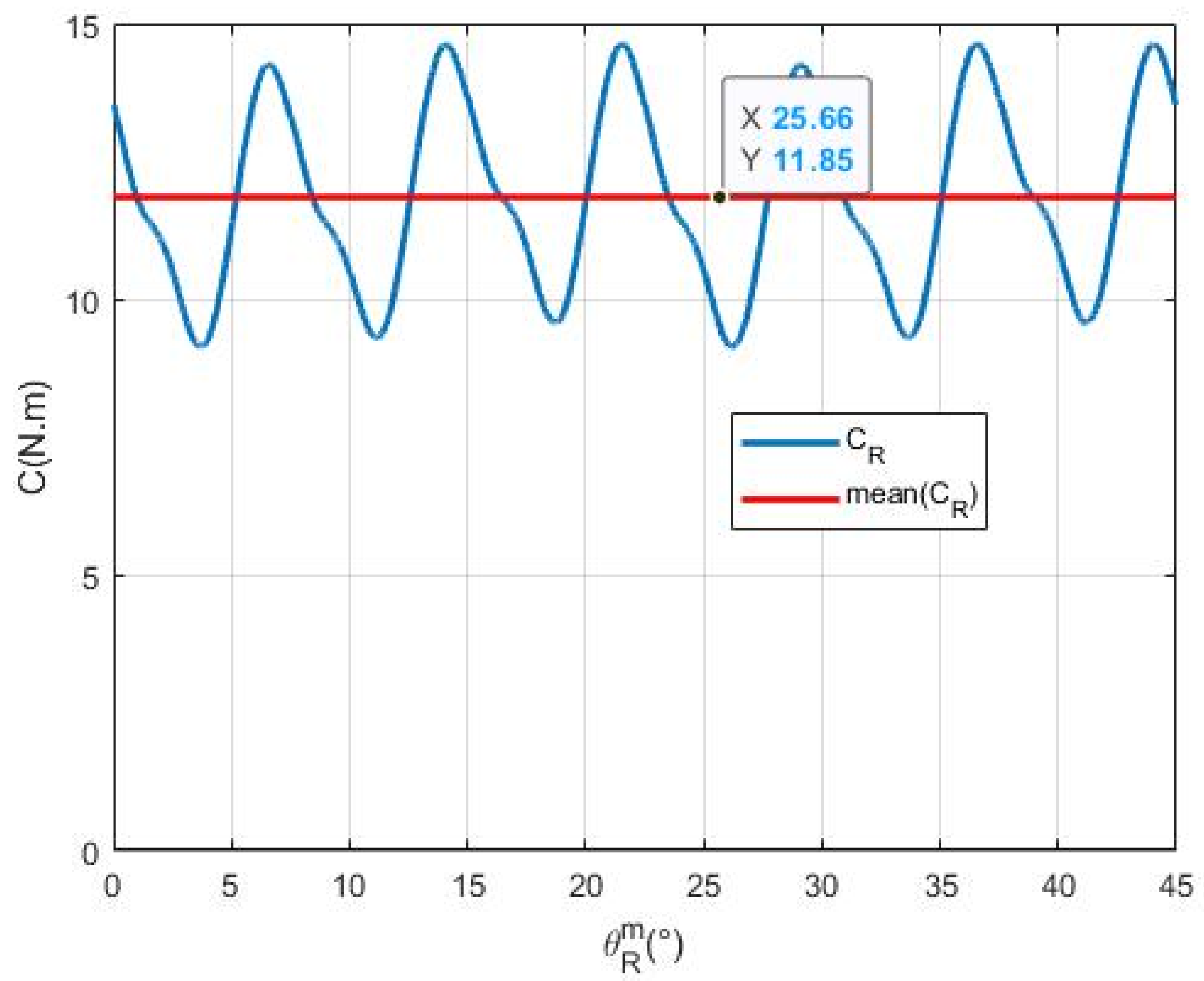
Once the entire set of parameters is established, the general electromechanical model facilitates quick and accurate motor analyses, especially the precise and quick replication of torque ripples. The outcomes demonstrate the benefits and drawbacks of the DQ model, which is the most popular electric motor model. It can precisely determine the mean torque value, but is unable to reproduce torque ripples. The DQ model’s capacity to determine the optimal torque per ampere for STAFPM motors is confirmed by the suggested general model. Consequently, a sizing model that can quickly and precisely determine the DQ model’s parameters is required to size STAFPM motors.

References

1. Gadiyar, N.; Van Verdeghem, J.; Severson, E.L. A Review of Axial Flux Permanent Magnet Machine Technology. IEEE Trans. Ind. Appl. 2023, 59, 3920–3933. [Google Scholar] [CrossRef]
2. Shi, Z.; Sun, X.; Yang, Z.; Cai, Y.; Lei, G.; Zhu, J.; Lee, C.H.T. Design Optimization of a Spoke-Type Axial-Flux PM Machine for In-Wheel Drive Operation. IEEE Trans. Transp. Electrif. 2024, 10, 3770–3781. [Google Scholar] [CrossRef]
3. Zhao, F.; Lipo, T.A.; Kwon, B.-I. A Novel Dual-Stator Axial-Flux Spoke-Type Permanent Magnet Vernier Machine for Direct-Drive Applications. IEEE Trans. Magn. 2014, 50, 8104304. [Google Scholar] [CrossRef]
4. Bilal, M.; Ikram, J.; Fida, A.; Bukhari, S.S.H.; Haider, N.; Ro, J. Performance Improvement of Dual Stator Axial Flux Spoke Type Permanent Magnet Vernier Machine. IEEE Access 2021, 9, 64179–64188. [Google Scholar] [CrossRef]
5. Gieras, J.F.; Wang, R.J.; Kamper, M.J. Principles of AFPM Machines. In Axial Flux Permanent Magnet Brushless Machines; Springer Science & Business Media: Berlin/Heidelberg, Germany, 2008. [Google Scholar]
6. Tessarolo, A.; Mezzarobba, M.; Menis, R. Modeling, Analysis, and Testing of a Novel Spoke-Type Interior Permanent Magnet Motor with Improved Flux Weakening Capability. IEEE Trans. Magn. 2015, 51, 8103910. [Google Scholar] [CrossRef]
7. Jiang, M.; Niu, S. Novel Mechanical Flux-Weakening Design of a Spoke-Type Permanent Magnet Generator for Stand-Alone Power Supply. Appl. Sci. 2023, 13, 2689. [Google Scholar] [CrossRef]
8. Krause, P.C.; Wasynczuk, O.; Sudhoff, S.; Pekarek, S. Reference-Frame Theory. In Analysis of Electric Machinery and Drive Systems; Published by John Wiley & Sons, Inc.: Hoboken, NJ, USA, 2013; ISBN 9781118024294. [Google Scholar]
9. Mohammadi, A.S.; Trovão, J.P. A Comparison of Different Models for Permanent Magnet Synchronous Machines: Finite Element Analysis, D-Q Lumped Parameter Modeling, and Magnetic Equivalent Circuit. In Proceedings of the 2019 IEEE 28th International Symposium on Industrial Electronics (ISIE), Vancouver, BC, Canada, 12–14 June 2019; pp. 197–202. [Google Scholar] [CrossRef]
10. Zarate, S.; Almandoz, G.; Ugalde, G.; Poza, J.; Escalada, A.J. Extended DQ model of a Permanent Magnet Synchronous Machine by including magnetic saturation and torque ripple effects. In Proceedings of the 2017 IEEE International Workshop of Electronics, Control, Measurement, Signals and Their Application to Mechatronics (ECMSM), Donostia, Spain, 24–26 May 2017; pp. 1–6. [Google Scholar] [CrossRef]
11. Mohammed, O.A.; Liu, S.; Liu, Z. Physical Modeling of PM Synchronous Motors for Integrated Coupling with Machine Drives. IEEE Trans. Magn. 2005, 41, 1628–1631. [Google Scholar] [CrossRef]
12. Filho, C.; de Alvarenga, B.P.; de Paula, G.T. On-Load Apparent Inductance Derivative of IPMSM: Assessment Method and Torque Estimation. IEEE Trans. Magn. 2020, 56, 8100610. [Google Scholar] [CrossRef]
13. Zhu, Z.Q. A simple method for measuring cogging torque in permanent magnet machines. In Proceedings of the 2009 IEEE Power & Energy Society General Meeting, Calgary, AB, Canada, 26–30 July 2009; pp. 1–4. [Google Scholar] [CrossRef]
14. Yankov, D.; Grigorova, T.; Maradzhiev, I. Simulation and Experimental Study of Static Torque Characteristics of a 12/8 Three-Phase SRM. In Proceedings of the 2023 18th Conference on Electrical Machines, Drives and Power Systems (ELMA), Varna, Bulgaria, 29 June–1 July 2023; pp. 1–4. [Google Scholar] [CrossRef]
15. Heins, G.; Thiele, M.; Brown, T. Accurate Torque Ripple Measurement for PMSM. IEEE Trans. Instrum. Meas. 2011, 60, 3868–3874. [Google Scholar] [CrossRef]
16. Pouramin, A.; Dutta, R.; Farshadnia, M.; Rahman, M.F. A Standstill Method to Measure Electromagnetically Induced Torque Ripple of Permanent Magnet Synchronous Machines. IEEE Trans. Instrum. Meas. 2020, 69, 7627–7635. [Google Scholar] [CrossRef]
17. Song, S.; Ge, L.; Ma, S.; Zhang, M.; Wang, L. Accurate Measurement and Detailed Evaluation of Static Electromagnetic Characteristics of Switched Reluctance Machines. IEEE Trans. Instrum. Meas. 2015, 64, 704–714. [Google Scholar] [CrossRef]
18. Ait-gougam, Y.; Ibtiouen, R.; Touhami, O.; Louis, J.-P.; Gabsi, M. Inverse modelling and pulsating torque minimization of salient pole non-sinusoidal synchronous machines. Electr. Power Syst. Res. 2008, 78, 88–96. [Google Scholar] [CrossRef]
19. Mrad, A. Moteur à Flux Axial à Aimants Permanents et à Concentration de Flux: Réalisation, Mesure de Paramètres Statiques et Modèle Numérique 3D. Ph.D. Thesis, Ecole Doctorale GEETS, Université de Toulouse, Toulouse, France, 2022. [Google Scholar]
20. Closa, D. Conception, Réalisation et Essais de Machines à Aimants Permanents et Commutation Electronique à Encombrement Axial Réduit. Ph.D. Thesis, Ecole Doctorale de Génie Electrique, Institut National Polytechnique de Toulouse, Toulouse, France, 1988. [Google Scholar]
21. Gallicchio, G.; Palmieri, M.; Grasso, E.; Nienhaus, M.; Cupertino, F. Inductances Computation Using Finite Element Analysis for PMSM Sensorless Control. In Proceedings of the 2020 IEEE International Conference on Power Electronics, Drives and Energy Systems (PEDES), Jaipur, India, 16–19 December 2020; pp. 1–6. [Google Scholar] [CrossRef]
22. de Paula, G.T.; de A. Monteiro, J.R.B.; de Alvarenga, B.P.; de Almeida, T.E.P.; Pereira, W.C.A.; de Santana, M.P. On-Load Back EMF of PMSM Using Maxwell Stress Tensor. IEEE Trans. Magn. 2018, 54, 8104115. [Google Scholar] [CrossRef]
23. Huang, S.; Chen, Z.; Huang, K.; Gao, J. Maximum torque per ampere and flux-weakening control for PMSM based on curve fitting. In Proceedings of the 2010 IEEE Vehicle Power and Propulsion Conference, Lille, France, 1–3 September 2010; pp. 1–5. [Google Scholar] [CrossRef]
24. Caruso, M.; Di Tommaso, A.O.; Miceli, R.; Nevoloso, C.; Spataro, C.; Trapanese, M. Maximum Torque per Ampere Control Strategy for Low-Saliency Ratio IPMSMs. Int. J. Renew. Energy Res. IJRER 2019, 9, 374–383. [Google Scholar]
Figure 1. STAFPM motor: (a) rotor; (b) stator [19].
Electricity 06 00024 g001
Figure 2. (a) Front view; (b) side view of the experimental test bench [19].
Electricity 06 00024 g002
Figure 3. Types of supply and phases connections: (a) single-, (b) double-, and (c) three-phase supply.
Electricity 06 00024 g003
Figure 4. Example of the output voltage delivered by the force sensor.
Electricity 06 00024 g004
Figure 5. Example of the torque applied on the rotor corresponding to Figure 4.
Electricity 06 00024 g005
Figure 6. Numerical treatments applied to the torque: (a) offset applied; (b) equalization along horizontal and vertical axes.
Electricity 06 00024 g006
Figure 7. Rotor torque over one mechanical period in function of rotor position.
Electricity 06 00024 g007
Figure 8. Saliency torque due to different current values (25 N force sensor).
Electricity 06 00024 g008
Figure 9. Self-inductances variations for different current values.
Electricity 06 00024 g009
Figure 10. Static torque without permanent magnet and double-phase supply with two different current values (25 N force sensor).
Electricity 06 00024 g010
Figure 11. 2 C R 23 θ R m / I c 2 for two different current values.
Electricity 06 00024 g011
Figure 12. Self- and mutual inductances calculated from harmonics and mean values.
Electricity 06 00024 g012
Figure 13. The measured cogging torque (25 N force sensor).
Electricity 06 00024 g013
Figure 14. Measured e.m.f. at a rotational speed of 400 rpm.
Electricity 06 00024 g014
Figure 15. Derivatives of the no-load fluxes in function of rotor position.
Electricity 06 00024 g015
Figure 16. No-load fluxes in function of rotor position calculated from their harmonics.
Electricity 06 00024 g016
Figure 17. Measured (25 N force sensor) and calculated saliency torque for I C = 2   A .
Electricity 06 00024 g017
Figure 18. Single-phase supply: measured (100 N force sensor) and calculated torques for: (a) I C = 1.0   A ; (b) I C = 3.6   A .
Electricity 06 00024 g018
Figure 19. Double-phase supply: measured (100 N force sensor) and calculated torques for I C = 2.0   A .
Electricity 06 00024 g019
Figure 20. Three-phase supply: measured (100 N force sensor) and calculated torques for I C = 2.6   A .
Electricity 06 00024 g020
Figure 21. DQ0 components of the no-load flux.
Electricity 06 00024 g021
Figure 22. The direct inductance L D θ R m and the quadrature inductance L Q θ R m for: (a) α = 30 ° ; (b) α = 120 ° .
Electricity 06 00024 g022
Figure 23. Torque and electromagnetic torque versus α .
Electricity 06 00024 g023
Figure 24. C R θ R m for α = α o p t = 93.3 ° .
Electricity 06 00024 g024