Abstract
In the future, higher penetrations of electrical loads in low-voltage distribution grids are to be expected. To prevent grid overload, a possible solution is coordination of controllable loads. Typical examples might be charging of electric vehicles or operation of electric heat pumps. Such loads are associated with specific requirements that should be fulfilled if possible. However, at the same time, a safe grid operation must be ensured. To this end, a corresponding optimal power flow optimization problem might be formulated and solved. This article gives a comprehensive review of the state of the art of optimal power flow formulations. It is investigated which constraint handling techniques are used and how hyper parameters are tuned when solving optimal power flow problems using metaheuristic solvers and how controllable loads and fluctuating renewable production are incorporated into optimal power flow formulations. Therefore, the literature is reviewed for pre-defined criteria. The results show possible gaps to be filled with future research: extended optimal power flow formulations to account for controllable loads, investigation of effects of choosing constraint handling techniques or hyper parameter tuning on the performance of the metaheuristic solver and automated methods for determining optimal values for hyper parameters.
1. Introduction
Higher penetrations of electrical loads—like charging stations for charging electric vehicles or electrical heat pumps for heating houses—will lead to higher electrical loads in future electrical low-voltage distribution grids. In addition to this, more fluctuating renewable generators, like photovoltaic power systems, will also need to be integrated in these distribution grids. Existing grids might at some point be over-loaded by these additional electrical loads and fluctuating renewable generators. One possible solution to prevent this overload might be to reinforce existing distribution grids or build new ones. However, this might take a long time and also come along with high costs. Another solution to prevent this overload might be the coordination of those additional electrical loads—given those loads are controllable [1]. Examples for these kinds of loads might be charging stations to charge electric vehicles (EVs) or electrical heat pumps together with thermal energy storages.
As a part of the EU-project ECS4DRES, algorithms to coordinate multiple controllable loads in low-voltage distribution grids are to be developed. The goal is to utilize existing low-voltage distribution grids as much as possible so as to fit in as many controllable loads as possible within the existing grid. This goal is to be achieved by optimal coordination of those controllable loads. This way, the requirements associated with those loads (for example, desired state of charge and time to finish an EV charging process or covering thermal demands using electrical heat pumps) should be fulfilled if possible. If the grid is already too congested to fulfil all those requirements, at least a non-discriminatory distribution of electrical energy is to be achieved. At the same time, however, violation of physical grid constraints must be avoided.
In a predecessor project, this has already been achieved for coordinating multiple EVs charging along a grid line [1]. However, this has been achieved only for the assumption of a single grid line and other simplifying assumptions, like only considering real parts of impedances. Using predictions for non-controllable loads (the majority of devices in typical households), an optimal “charging schedule” can be computed as a result of solving the associated optimization problem. However, in reality, there will never be perfect predictions for any load. So, when new measurement values arrive—indicating deviation of actual load profiles from the predicted ones—a correspondingly updated optimization problem is formulated and solved. The solution to this updated optimization problem is an updated charging schedule that incorporates the new situation in the grid. This procedure, however, requires a fast solution to the optimization problem to be able to react to new measurement values in time. Due to the aforementioned assumptions, the optimization problem could be formulated as a linear problem. This allowed a fast solution for the global optimum using the simplex algorithm.
However, when using more realistic formulations, this will lead to more complex optimization problems. Such problems are known as optimal power flow (OPF) problems.
These OPF problems are non-linear, non-convex (this will be discussed in Section 3.1), and generally time intensive to solve—especially if integer or binary variables are involved in the OPF formulation (which might be the case for realistic modeling of certain components, like minimum/maximum output power of heat pumps) [2]. Analytical solvers—typically based on gradient descent methods—cannot be guaranteed to find the global optimum of such non-convex optimization problems and might take very long to converge [3]. Alternative solutions for OPF problems are therefore being researched. One very prominent approach is the usage of metaheuristics (this will be discussed in Section 3.2) for solving such OPF problems. These metaheuristics cannot be guaranteed to find the global optimum—however, classical analytical solvers also cannot—and can also find solutions quicker than those analytical solvers [4]. Often, these metaheuristics are based on swarm intelligence—taking inspiration from natural swarms like birds or ants—or also from evolution.
However, metaheuristics only solve unconstrained optimization problems [5]—so they can only be used to maximize or minimize a certain objective function without consideration of constraints. But OPF problems consist of many constraints (to ensure proper operation of the considered grid without overload or also proper operation of connected loads and keeping other requirements). So, in order to utilize metaheuristics for solving OPF problems, one first has to ensure that constraints are being taken into account. Therefore, there are constraint handling techniques [6]. In addition to this, metaheuristics have certain hyper parameters to be tuned [7]. These hyper parameters determine the “performance” of the metaheuristic—how fast the metaheuristic converges to a result and also the optimality of that result. So, in addition to constraint handling techniques, one also needs to tune hyper parameters in order to utilize metaheuristics for solving OPF problems (or generally optimization problems) and to achieve results as optimal as possible.
The goal of this review paper is not to show how the mentioned optimization problem formulation for controlling multiple controllable electrical loads in electrical low voltage distribution grids might look like and also not to give an overview of metaheuristics typically used for solving these kind of optimal power flow problems; [8] already gives an up-to-date comprehensive overview. However, in [8], it is not mentioned which constraint handling techniques were used in the reviewed articles or how hyper parameters of the metaheuristics were tuned. In contrast, an overview of available constraint handling techniques is given in [5] but without connection to OPF problems. So, the goal of this review paper is to show what constraint handling techniques are typically used when solving OPF problems using metaheuristics and how hyper parameters of those metaheuristics are tuned. In addition to this, the inclusion of controllable loads and fluctuating renewable generation, like wind and PV, is examined. Therefore, a comprehensive literature review is carried out.
The remainder of this review is structured as follows: In Section 2, the methodology for the literature review is described, showing how research was conducted and which criteria are important for the review. Section 3 describes some background regarding optimal power flow, metaheuristics, and constraint handling techniques—but just as much as needed to be self-contained. In Section 4, the results of the literature review are shown. Finally, in Section 5, the results are discussed and a conclusion is drawn.
2. Materials and Methods
The relevant literature is found using scientific literature databases. The databases considered for this review are:
- Scopus,
- IEEE Xplore and
- IET Digital Library
In these literature databases, the results are further refined using advanced queries. To keep the relevant literature up to date, the results are constrained to years from 2016 to 2024 (both included). Furthermore, only open accessible (gold open access) articles are considered. Relevant keywords are:
- “optimal power flow”,
- “meta heuristic” and
- “constraint handling technique”
The so-found articles afterwards are scanned for certain criteria:
- the used optimal power flow formulation (what is the objective of optimization?)
- the used metaheuristic
- the used constrained handling technique
- the used technique for tuning hyper parameters
- are violations of constraints (node voltages, transformer load) monitored?
- are controllable loads or fluctuating renewables considered?
- is a multiple timestep or only a single timestep problem considered?
- which grid topology, at which voltage level, is considered?
- how is the load flow formulated?
3. Background
It is not the scope of this article to give a comprehensive overview of existing metaheuristics and constraint handling techniques or the concept of optimal power flow. However, for the sake of being self-contained, these points are introduced here.
3.1. Optimal Power Flow
Optimal power flow problems are a family of optimization problems that all try to optimize power flows in an electrical grid. There might be many different goals for this optimization—each associated to a corresponding objective function. However, all formulations have one thing in common: a safe operation of the electrical grid is to be ensured; for example, power balance and keeping equipment in the grid in tolerable operational limits. This leads to corresponding constraints. The decision variables are made up of controllable variables and state variables. The control variables can be directly acted upon by grid operators: for example, the output power of controllable, thermal power plants or the tap setting of transformers. The state variables are coupled to the control variables via constraints that describe the operation of the grid. For example, node voltages or voltage angles depend on the power drawn from or fed into the grid. Parameters are given as demands that need to be fulfilled and information about the grid itself—which is gathered in the form of an admittance matrix, reflecting the physical properties of the grid.
By the nature of physical laws describing the grid operation, these optimal power flow optimization problems are [9]
- non-linear:
- either the objective function or constraints cannot be formulated exclusively as a linear combination of the decision variables. For example, is linear, but is not linear. Non-linearity might lead to non-convexness.
- non-convex:
- there is not one global optimum, but many local optima (in which solvers might “get stuck”); an example is given in Figure 1.
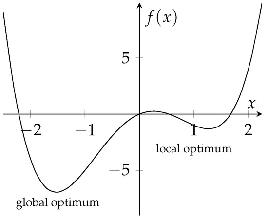 Figure 1. Example graph of a non-convex function; here, , with local and global optima for minimization. Solvers might “get stuck” in local optima. For ease of comprehension and visualization, this is just a one-dimensional example. However, the same also holds for n-dimensional examples.
 - constrained:
- there are constraints involved in the formulation of the optimization problem, for example, .
A generic non-linear, constrained OPF optimization problem might look like what is shown in Equation (1):
Here, is the objective function—in the context of OPF, this might typically be some kind of cost metric to be minimized. g and h are inequality and equality constraints, respectively, and I and J are the corresponding sets of all inequality and equality constraints, respectively. is a vector of decision variables that may be sub divided into a vector of control variables and a vector of state variables , such that [9]. Control variables are those variables that can be directly acted upon—for example, active power output of thermal generators, tap settings of tap changing transformers, or reactive power fed by shunt var compensators. State variables, on the other hand, are those variables that are affected by the settings of control variables—for example, node voltage magnitudes and angles or apparent powers flowing through the lines.
3.1.1. Ways to Calculate Load Flow
To determine optimal power flow, it is important to calculate node voltages and currents on the lines in dependence of load/generation in the grid. This is usually referred to as load flow. From the view point of the optimization problem, the load flow links the state variables to the control variables. In general, there are two ways to calculate this load flow, which differ in their applicability: (1) the “complete” power flow is valid for arbitrary grid topologies, and (2) the forward-backward-sweep, which is only valid for radial, non-meshed grids.
Complete Power Flow
The formulation for the complete power flow is valid for arbitrary grid topologies. It is based on the nodel voltage analysis [10]. Provided information on grid topology, given in the form of an admittance matrix for a grid consisting of n buses and currents drawn from/fed into the grid at the n nodes, the voltages at those n nodes can be calculated according to Equation (2).
Typically, admittances will be given in cartesian form such that , where is the conductance and is the susceptance of the -th element of the admittance matrix. Node voltages are typically given in polar form such that , where is the magnitude and is the angle of voltage at node i. Formulating active and reactive power balances for each node in the grid will lead to formulations as given in Equations (3) and (4):
where N is the set of all nodes in the grid. and denote active power fed into and taken from the grid at node i, respectively. The remaining term calculates the active power flowing through the lines attached to node i.
where and denote reactive power fed into and taken from the grid at node i, respectively. The remaining term calculates the reactive power flowing through the lines attached to node i.
Forward-Backward-Sweep
The forward-backward-sweep is only valid for radial grids with no meshes. It is an iterative calculation [11]. Each iteration consists of a forward sweep and a backward sweep. In the first iteration, it is assumed that all node voltage magnitudes are at the nominal level. Given active and reactive power demands/generations at the nodes as well as assumed voltages at the nodes, active and reactive currents flowing out/into the grid at those nodes are computed according to Equation (5).
Now, in the forward sweep, starting at the last node moving towards the first node, the currents flowing on the lines are calculated according to Equation (6):
In the following backward sweep, starting at the fist node moving towards the last node, the node voltages are updated using the previously calculated line currents and line impedances according to Equation (7):
This will result in node voltages lower than the ones initially assumed. In the following iterations, this will lead to accordingly updated line currents. The end of the iterations is reached once the difference in node voltages between two consecutive iterations is smaller than a certain delta. A visualization of a radial grid line and corresponding quantities is given in Figure 2.

Figure 2.
A grid line and corresponding quantities for calculating forward-backward-sweep.
3.1.2. Typical Objectives for Optimal Power Flow Problems
There is not the one and only OPF formulation; there may be different objectives that lead to different formulations of the objective function. Some objectives commonly found in the literature are summarized here. At the end of this subsection will be an outlook on what a formulation for an objective for coordinating controllable loads might look like.
Minimizing Fuel Costs
The goal here is to minimize the fuel costs for thermal power plants to supply all the required load. This is formulated according to Equation (8):
where is the set of all controllable generators attached to the grid. , , and are coefficients describing the fuel cost for the i-th generator with output power .
Minimizing Active Power Losses
Here, the objective is to minimize active power losses in all transmission lines of the grid. This is formulated according to Equation (9)
where and are voltage magnitudes as nodes i and j, respectively. Similarly, and are voltage angles, and is the conductance of the -th element of the system admittance matrix . N is the set of nodes in the grid.
Minimizing Voltage Deviations
The objective is to minimize voltage deviations across all nodes in the considered grid. This is formulated according to Equation (10)
where is the voltage magnitude (in p.u.) at node i and N is the set of nodes in the grid.
Outlook: Possible Objective for Coordinating Controllable Loads
An objective for coordinating multiple controllable loads, as mentioned in the introduction (e.g., charging EVs or electrical heat pumps), might, for example, look like Equation (11)
Here, and are the sets of nodes with a wallbox and a heat pump connected to it, respectively. is the charging power of the EV charging at node i and is the amount of thermal energy missing to fulfil the thermal demand of the houshold at node i. p is an according penalty, which will help minimize . Of course, this will also require corresponding equality constraints for balancing thermal demands of households. However, this is just supposed to be a quick outlook, so these additional constraints will not be described here.
3.1.3. Equality Constraints
Equality constraints ensure power balance in the grid, thus enforcing all the required demand is fulfilled by appropriate generation. There are two separate sets of equality constraints: one set for active power balance and another set for reactive power balance. Those constraints were already described in Equations (3) and (4) in Section 3.1.1.
3.1.4. Inequality Constraints
Inequality constraints ensure safe operation of the grid, keeping all decision variables in tolerable operating limits. This way, it can be ensured that no grid infrastructure is damaged and a safe grid operation is achieved. These constraints are formulated according to Equations (12)–(17).
Here, , , and are active power, reactive power, and voltage of the i-th generator and is the set of all generators. is the tap setting of the i-th transformer and is the set of all generators. and are voltage at i-th node and apparent power flowing through the i-th line, respectively. N and L are the sets of all nodes and all lines, respectively.
3.2. Population-Based Metaheuristics and Why to Use Them
Population-based metaheuristics can be used as an alternative to a classical solver. So, a metaheuristic instead of a classical solver is used to solve an optimization problem. To optimally control multiple controllable electrical loads in a low-voltage distribution grid, a corresponding OPF optimization problem can be formulated and solved. As described in Section 3.1, these OPF problems are constrained, non-linear, and non-convex and thus generally hard to solve. If integer or binary variables are involved (which might be the case for realistic modeling of components like heat pumps), the time for classical solvers to converge rises exponentially with the number of binary variables [2]. In addition to this, classical solvers cannot be guaranteed to find the global optimum of non-convex problems [12]. Metaheuristic solvers also cannot be guaranteed to find the global optimum of such problems. However, metaheuristics might converge faster than classical solvers. So, metaheuristics might be a viable alternative to classical solvers when it comes to large, non-convex optimization problems including integer or binary variables. Figure 3 shows the connection between the physical grid (including devices to be optimally coordinated), the corresponding OPF formulation, and the metaheuristic used to solve the OPF problem.
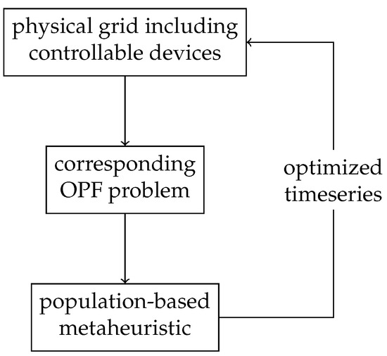
Figure 3.
Connection between physical grid, corresponding OPF formulation, and the metaheuristic solver.
In contrast to trajectory-based metaheuristics, which only consider one solution per Iteration (just like classical solvers), population-based metaheuristics consider multiple solutions per iteration, where each solution equals one member of the population. So, for a population-based metaheuristic, a population is initialized. Each member of this population represents one possible solution to the considered OPF problem. So, for an OPF problem with n decision variables, one member represents one point in an n-dimensional search space. So, each member can be thought of as a vector consisting of n elements, where each element represents a concrete value for one of the n decision variables: . To draw a connection to the grid, one might think of active/reactive output of controllable generators ( or ), transformer tap settings (), node voltages (), or line apparent powers (), for example, as depicted for a simple grid in Figure 4.

Figure 4.
A simple example grid to show control variables (in red) and state variables (in blue) that constitute a complete vector of decision variables. Typically, each member in a population-based metaheuristic represents one vector of control variables.
Typically, control variables are used to make up the members of the population, such that each member represents one vector of concrete values for those control variables [13,14]. So, for the sample grid in Figure 4, each member of the population consists of concrete numerical values for each of the control variables, for example:
Each of these members can be assigned a value of the objective function, evaluated at the position of this member: .
Particle swarm optimization (PSO), first described by [15] in 1995, serves as an example. Based on the swarm behavior of, for example, birds, the members of the population “navigate through the topology of the objective function”. Each member updates its current position based on its own best position found so far and the best position found by the entire population so far. According to Equation (18), the “velocity” of member i at iteration t is updated:
where , , and are referred to as inertia, cognitive parameter, and social parameter, respectively. These factors determine how much the members orient on their own best solutions or the whole population’s best solutions found so far. Thus, these parameters have influence on convergence of the PSO and need to be tuned for proper performance. These parameters are also referred to as hyper parameters. A stochastic element is introduced with rand, which stands for a random number. Then, the new position of each member is calculated according to Equation (19):
This way, the members of the population explore the landscape of the objective function. Depending on the hyper parameter settings, the members of the population may take different paths, which might lead to more exploration of their environment or exploitation of discovered optima. With help of the stochastic element, members may also be able to leave local optima in case they become stuck. However, constraints are not yet considered. So, the optimization problem (which represents the physical grid, see Figure 3) cannot be solved while satisfying all the constraints yet. Therefore, there are constraint handling techniques.
3.3. Constraint Handling Techniques
As already stated in Section 3.2, metaheuristics can only optimize unconstrained optimization problems. However, many problems—including OPF—need constraints to be modeled realistically. Therefore, constraint handling techniques (CHTs) are used to account for constraints that are violated by proposed solutions.
3.3.1. Static Penalty Function
With help of a static penalty function, the violation of constraints—introduced by solutions proposed by the metaheuristic—can be integrated into the objective function. This way, such solutions are penalized and less attractive [6]. For a constrained optimization problem as shown in Equation (1), the penalized objective can be written as Equation (20):
where and are penalty factors for inequality and equality constraints, respectively. These penalty factors determine how much constraint violations are penalized. The penalty factors also need to be tuned to ensure good performance of the metaheuristic solver. In general, constraints that are deemed more important are associated with a higher penalty factor. The penalized objective is usually referred to as “fitness”.
3.3.2. Superiority of Feasible Solution
With the help of feasibility rules, as described in [16], infeasible solutions can be excluded from the population. Here, a tournament selection operator is used, where two solutions are compared at a time. The “winning” solution to be kept in the population is determined as follows:
- feasible solutions are always preferred to infeasible ones,
- given two feasible solutions, the one with better objective value is preferred, and
- given two infeasible solutions, the one with less constraint violation is preferred.
4. Results of the Literature Review
Including all the relevant keywords in the query only led to two articles in Scopus and zero articles in IEEE Xplore. However, by skipping the keyword “constraint handling technique”, already 100 articles were found in Scopus and 30 articles in IEEE Xplore. However, some articles were listed in both Scopus and IEEE Xplore. Among those articles, the ones relevant have been scanned for the relevant criteria, as outlined in Section 2. The results are listed in Table 1, Table 2, Table 3, Table 4, Table 5 and Table 6. Each of the criteria mentioned in Section 2 is devoted a separate column in Table 1, Table 2, Table 3, Table 4, Table 5 and Table 6. Inside those tables, only abbreviations are used. Here is an overview of the used abbreviations:

Table 1.
Results of reviewing the literature for relevant criteria.
Table 2.
Results of reviewing the literature for relevant criteria; continuation of Table 1.
Table 3.
Results of reviewing the literature for relevant criteria; continuation of Table 2.
Table 4.
Results of reviewing the literature for relevant criteria; continuation of Table 3.
Table 5.
Results of reviewing the literature for relevant criteria; continuation of Table 4.
Table 6.
Results of reviewing the literature for relevant criteria; continuation of Table 5.
- MH:
- The metaheuristic used to solve the OPF problem (as it is not the scope of this review to give a comprehensive overview of metaheuristics, they are just mentioned for the sake of completeness. A prepender (I) means an “improved” version of the base algorithm—according to the authors of the respective article). The following values might appear in this column: GWO: Gray Wolf Optimizer, HHO: Harris Hawk Optimizer, MSA: Moth Swarm Algorithm, SSA: Salp Swarm Algorithm, MRF: Manta Ray Foraging Algorithm, SGA: Search Group Algorithm, JAYA: Jaya Algorithm, GA: Genetic Algorithm, SGO: Social Group Optimization, TSO: Transient Search Optimization, GMO: Geometric Mean Optimization, FFO: Firefly Optimization, TFW: Turbulent Flow of Water Optimization, ACO: Ant Colony Optimization, DE: Differential Evolution, CO: Coati Optimization, WSO: War Strategy Optimization, FHO: Fire Hawk Optimization, FPA: Flower Pollination Algorithm, SOA: Skill Optimization Algorithm, PSO: Particle Swarm Optimization, ABC: Artificial Bee Colony Optimization, MGO: Mountain Gazelle Optimizer, GBE: Gradient Bald Eagle Search, BSA: Bird Swarm Algorithm, HSA: Harmony Search Algorithm, GSA: Gravitational Search Algorithm, WHA: Wild Horse Optimization, SFS: Stochastic Fractal Search, MFA: Moth Flame Algorithm, MVO: Multi-Verse Optimization, WOA: Whale Optimization Algorithm, SBB: Satin Bowerbird Optimization, ALO: Ant Lion Optimizer, KHA: Krill Herd Algorithm, AO: Aquila Optimizer, SMO: Slime Mould Optimizer, CO: Coyote Optimization, GHO: Grasshopper Optimization, POA Peafowl Optimization, HGS: Hunger Games Search, AHB: Artificial Hummingbird Optimization, ISA: Interior Search Algorithm, EO: Equilibrium Optimizer, VND: Variable Neighbourhood Descent Algorithm, SFL: Shuffled Frog Leaping Optimization, TSA: Tree Seed Optimization, SOS: Symbiotic Organisms Search Algorithm, GNDO: Generalized Normal Distribution Optimizer, COO: Coot Optimizer, AVO: African Vultures Optimization, HMO: Homonuclear Molecules Optimization, CSA: Cuckoo Search Algorithm AOA: Arithmetic Optimization Algorithm, CHIO: Coronavirus Herd Immunity Optimizer, COA: Chimp Optimization Algorithm, EDM: Empirical Discrete Metaheuristic, CSM: Coordinate Search Method, SuSA: Super Spherical Algorithm, ROA: Rider Optimization Algorithm, WCA: Water Cycle Algorithm.
- CHT:
- The used constraint handling technique to ensure constraints are taken into account when solving the OPF problem with a metaheuristic solver. The following values might appear in this column: SPF: static penalty function, SFS: superiority of feasible solution, LPIM: linear penalty incremental method, ACC: archive-based constraint correction, SAP: self adaptive penalty, ROP: robust oracle penalty, GOF: Graded Objective Functions, N!: not even mentioned.
- HPT:
- Hyper parameter tuning to ensure good convergence of the meat heuristic when solving the OPF problem. The following values might appear in this column: SV: at least static values are given, TE: trial and error, N!: not even mentioned.
- ObjOPF:
- The objective of the OPF problem. The following values might appear in this column: MFC: minimize fuel costs, MFC*: minimize fuel costs (considering valve point effect), MIO: minimize invest and operational costs, MOC: minimize operational costs, MIC: minimize investment costs, MVD: minimize voltage deviation, MPL: minimize active power losses, MPL*: minimize reactive power losses, VSI: maximize voltage stability index, ME: minimize emissions, MES: minimize energy not served, MCC: minimize congestion costs, MPP: maximize PV penetration, TLL: maximize total loadability limit, MCP: minimize costs for changing power output, MSR: minimize system risk, MPI: minimize power import.
- CVM:
- Whether constraint violations are monitored; for example, node voltages or transformer load. The following values might appear in this column: NV: node voltages, N!: not even considered.
- MTC:
- Whether multiple time steps are considered for the formulation of the OPF problem. The following values might appear in this column: DHR: one day in hourly resolution, YHR: one year in hourly resolution, YMN: one year in mothly resolution N!: not considered.
- CLC:
- Whether controllable loads are considered in the OPF problem formulation (as opposed to just controllable thermal generators). The following values might appear in this column: EV: electric vehicles, Alu: Aluminium plant, N!: not considered.
- FRC:
- Whether fluctuating renewables are considered in the OPF problem formulation. The following values might appear in this column: PV: photovoltaic, WE: wind energy, HE: hydro energy, BG: Bio gas, N!: not considered.
- CGr:
- The grid considered in the study. The following values might appear in this column: ERG: existing real-world grid, TGr: test grid (like IEEE xxx-bus grids), N!: not even mentioned.
- GVL:
- The voltage level of the considered grid. The following values might appear in this column: HMV: high to medium-voltage (e.g., everything above low-voltage), LV: low-voltage, N!: not deducible.
- CRC:
- Whether the results of solving the OPF problem were compared when using different constraint handling techniques (yes or no).
- FLF:
- How the load flow is formulated. The following values might appear in this column: FB: forward-backward-sweep, PF: complete power flow, DLF: Distribution Load Flow Matrix, N!: not even mentioned.
4.1. Used Constraint Handling Techniques
Most of the reviewed articles use a static penalty function, as shown in Equation (20), to integrate constraint violation into the objective function; then, the resulting fitness function is optimized. Only very few articles use different constraint handling techniques. Also, many articles don’t even mention constraint handling techniques—even though they have to be used in order to achieve feasible solutions to OPF problems. The results are shown in Figure 5.
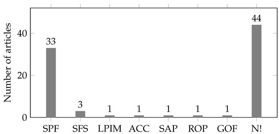
Figure 5.
Results of the literature review for used constraint handling techniques (SPF: static penalty function, SFS: superiority of feasible solution, LPIM: linear penalty incremental method, ACC: archive-based constraint correction, SAP: self adaptive penalty, ROP: robust oracle penalty, GOF: Graded Objective Functions, N!: not even mentioned).
A typical example for an article using static penalty function for handling constraints is [22]. Bounds of decision variables are formulated as inequality constraints. Violation of those bounds are penalized via penalty factors and added on top of the original objective function, as described by Equation (20).
Only one article compares the results of optimization for different constraint handling techniques: In [34], authors compare “superiority of feasible solution” and “self-adadptive penalty” for handling constraints as well as an ensemble of both methods. Optimizations are carried out on IEEE 30-, 57-, and 118-bus systems with either single or multiple objectives like minimizing fuel costs, power losses, or voltage deviations. A differential evolution was used for solving the OPF problem, combined with different CHTs. Statistical analyses of the objective function values are carried out using the Wilcoxon signed rank test. However, the results show that no single CHT is able to produce the best results for all considered cases.
Other CHTs like the linear penalty incremental method (LPIM), archive-based constraint correction (ACC), and robust oracle penalty (ROP) were only used very seldomly. In [21], the authors used LPIM and ACC as CHTs. Optimizations were carried out on IEEE 30- and 57-bus systems using a gray wolf optimizer based on symbiotic learning. Objectives of the OPF formulation were, for example, minimization of fuel costs, emissions, power losses, or voltage deviation—either considered as single objectives or multiple objectives via weighted sum. For constraint handling, the authors use a combination of LPIM and ACC, with LPIM as the primary CHT. After a certain number of iterations, ACC might be used as a secondary CHT, based on probability. In the LPIM, the penalty factors—as described in Equation (20)—are linearly increased with the number of iterations. Thus, in the first iterations, penalties are smaller, leading to more exploration, while at higher iterations, penalties are bigger, leading to more exploitation of found optima. In ACC, an archive stores solutions with the least constraint violations so far. In order for new solutions to enter this archive, their constraint violation must be less than those solutions stored in the archive.
In [33], the authors use a robust oracle penalty for handling constraints. A micro grid consisting of five nodes is considered for optimization. The objective of the OPF formulation is to minimize power import from the main grid. The authors do not expand on the explanation of ROP; however, further information can be found in [99]: ROP is based on only one parameter, the oracle. Ideally, this oracle is to be set slightly greater than the optimal feasible solution—which of course is not known beforehand. Starting with an initial guess, the oracle is updated each iteration, moving closer to an optimum, thus resulting in a kind of self-tuning effect. For further details, the reader is referred to [99].
Another approach is shown in [94], where a technique called “graded objective functions” is used. This way, constraints are converted into bounded objective functions. The main goal is to minimize power losses; however, constraints to prevent over-voltage and under-voltage are accordingly converted to objective functions. Based on their harmfulness, these objective functions are ordered and subsequently solved for: in a first stage, over-voltages are to be minimized, then in a second step, under-voltages are to be minimized. Finally, the power losses in the system are to be minimized. According to the authors, by employing the graded objective functions, “the probability of non-convergence, which can occur with advanced algorithms in certain situations, is minimized.” [94].
4.2. Used Techniques for Hyper Parameter Tuning
Many of the reviewed articles do not even mention how the hyper parameters for the metaheuristic solver were set. The other articles at least showed what values they have set for the hyper parameters of their used metaheuristic. Only three articles stated that “optimal” values for hyper parameters were determined based on trial and error. The results are shown in Figure 6.

Figure 6.
Results of the literature review for used hyper parameter tuning (SV: at least static values given, TE: trial and error, N!: not even mentioned).
In [67], an IEEE 30-bus grid is considered for optimization. The objectives of the OPF are to simultaneously minimize fuel costs and power losses in transmission lines. For solving the OPF problem, the authors use a hybrid of differential evolution and symbiotic organisms search. The authors state that the optimal hyper parameter settings were obtained “[a]fter several trial runs of the algorithm”.
In [75], IEEE 30- and 118-bus systems are considered for optimization. Here, the objectives of the OPF formulation include minimizing fuel costs, emissions, voltage deviation, and power losses in transmission lines. Manta ray foraging optimization is used to solve the OPF problem. According to the authors, “[t]he best solution (optimal values) for each parameter was chosen”. The authors provide a table with a testing range for each hyper parameter of different metaheuristics. However, it is not explained how the best solution was determined—probably also by trial and error in the given ranges.
4.3. Objectives of the Optimal Power Flow Formulation
Most of the reviewed articles consider minimization of power losses in transmission lines, voltage deviation, or fuel costs as objective. The results are shown in Figure 7. In most of the cases, either single objectives or multiple objectives are considered. That is the reason why the number of articles in Figure 7 sums up to more than the total number of reviewed articles.
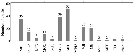
Figure 7.
Results of the literature review for used OPF objectives (MFC: minimize fuel costs, MFC*: minimize fuel costs (considering valve point effect), MIO: minimize invest and operational costs, MOC: minimize operational costs, MIC: minimize investment costs, MVD: minimize voltage deviation, MPL: minimize active power losses, MPL*: minimize reactive power losses, VSI: maximize voltage stability index, ME: minimize emissions, MCC: minimize congestion costs, MPP: maximize PV penetration, TLL: maximize total loadability limit).
In the case of multiple objectives, two options are possible. Either a weighted sum of the single objectives, which leads to a scalar multi-objective function, as is demonstrated, for example, in [39], or calculating a pareto front based on a vector-valued objective function, as, for example, described in [18]. The mostly used objectives are to minimize power losses in transmission lines, voltage deviation, or fuel costs for thermal generators. But also, sometimes objectives like minimizing congestion costs or increasing total loadability limit are included in OPF formulations. Most of the times, these objectives are achieved by corresponding coordination of controllable thermal units. But also sometimes, for example, placement or sizing of flexible AC transmission systems (FACTS) devices is used to achieve those objectives or distributed generation is considered.
In [35], different objectives like minimizing fuel costs, power losses in transmission lines, voltage deviations, and emissions or maximizing voltage stability index are considered. The authors consider different cases, either single objectives or multiple objectives as a weighted sum. This way, up to four objectives are considered simultaneously. Optimizations are carried out on IEEE 30-, 57-, and 18-bus systems using the moth swarm algorithm as a solver. The objectives are achieved using controllable thermal generators.
In [61], the authors consider different objectives like minimizing fuel costs, voltage deviation, active and reactive power losses in transmission lines or maximizing voltage stability index. However, here, only one objective at a time is considered. Optimizations are carried out for an IEEE 30-bus grid. A hybrid firefly particle swarm optimization is used to solve the OPF problem. Here, also controllable thermal generators are used to achieve the objectives.
In [49], the objectives of the OPF formulation are to minimize power losses in transmission lines and to maximize total loadability limit of the grid. Both objectives are considered simultaneously using a pareto front. The optimizations are carried out on an IEEE 30-bus grid. The authors use a genetic and a harmony search algorithm. The objectives are achieved by optimal placement and sizing of FACTS devices.
Similarly, in [57], the optimal placement and sizing of FACTS devices is used to achieve certain objectives. Here, this objective is to minimize investment and operating costs for those FACTs devices. In a first step, the optimal placement of those FACTS devices is manually determined. In a next step, the optimal sizing of those FACTS devices is determined using whale optimization. Here, IEEE 14- and 30-bus systems are considered for the optimization.
In [50], the objectives of the OPF formulation are to minimize fuel costs and power losses in transmission lines and maximize voltage stability index. The objectives are considered one at a time. Here, IEEE 30- and 118-bus grids are considered for the optimization. To solve the OPF problem, the authors use the Jaya algorithm. Using statistical analyses, also the effect of distributed generation on the performance of the solver is considered.
It is already noticeable here that none of the articles examined pursues the goal described in the introduction (to enable the coordination of as many controllable loads as possible, such as electric heat pumps and charging stations in existing low-voltage grids).
4.4. Methods for Formulating the Load Flow
In addition to the different objectives for the OPF problem, as mentioned in Section 4.3, there are also differences in the way that the load flow is incorporated into the OPF formulation. However, there are only two different approaches in the reviewed literature: (1) for radial, non-meshed grids, a forward-backward-sweep according to Equations (5)–(7) can be employed, or (2) for arbitrary (also meshed) grids, a “complete” power flow formulation according to Equations (3) and (4) can be employed. Finally, both formulations yield the state variables in dependence of the control variables. The results of the literature review are shown in Figure 8

Figure 8.
Results of the literature review for methods to formulate the load flow (FB: forward-backward-sweep, PF: full power flow, N!: not even mentioned).
Articles like ref. [63] or ref. [60] use the forward-backward-sweep because they only consider radial, non-meshed grids. In those grids, solving the forward-backward-sweep iterations converges faster than solving Gauss–Seidel or Newton–Raphson for the corresponding full power flow formulation. Most other articles that consider meshed grids have to use the full power flow formulation because meshed grids cannot be formulated using forward-backward-sweep.
However, there are also some articles that do not even mention how load flow is formulated, like ref. [30] or ref. [42]. Such papers just formulate balances for active and reactive powers but do not describe how this affects the load flow (there is no connection between control and state variables). Also, one article [53] describes both approaches, and it is not obvious which one is used (probably forward-backward-sweep because of the radial grid).
4.5. Consideration of Controllable Loads
Most of the reviewed articles consider the optimization of controllable, thermal generators. Only in four articles electric vehicles were considered—however, not as controllable load but just as additional load that has to be supplied. Only one article deviates from this pattern. All those articles have in common that demand for EV charging is determined by probability distribution functions. In [28], additional EV charging in IEEE 30-bus and IEEE 57-bus networks is considered. A certain penetration of EVs (and also PHEVs) with battery capacities and initial SOCs is assumed according to normal distributions. This results in an additional power demand added on top of residential load profiles. The OPF problem with objectives like minimization of fuel costs, voltage deviations, power losses, and maximization of voltage stability index is solved with an improved social group optimization. Since charging profiles are fixed in advance according to probability density functions, EV charging cannot be optimized anymore. Therefore, the work does not allow a coordination of EVs in the sense of controllable loads.
In [29], additional EV charging as well as fluctuating production of renewables is considered in an islanded AC-DC hybrid microgrid based on an IEEE 33-bus test grid. Production of renewables as well as demand for charging EVs are based on according probability distribution functions. Using Monte-Carlo simulations and a fast forward scenario reduction technique, additional loads and charging demands are projected over 24 h for multiple scenarios. The optimization with the objective of minimizing operational costs is carried out using a transient search optimization. Since charging profiles for EVs are calculated beforehand using probability density functions, for the optimization, those charging profiles are just fixed parameters and cannot be optimized. Thus, the work in this article does not allow a coordination of EVs in the sense of controllable loads.
In [47], EV charging and also vehicle-to-grid (V2G) together with fluctuating wind and PV production are considered in an IEEE 30-bus grid. Again, renewables production and EV load profiles are determined before the optimization according to given probability density functions obtained after multiple Monte-Carlo simulations. The objectives of the OPF formulation are to minimize power losses on transmission lines, voltage deviations, and total operation costs. A gradient bald eagle optimization is used for solving the OPF problem. Since the charging pattern for the EV is already predefined according to a given probability distribution, the EV charging cannot be optimized. Thus, also this work does not allow a coordination of EVs as controllable loads.
In [33], EV charging in a 5-bus microgrid is considered. There are also fluctuating PV production and other components like a storage in this micro grid. The goal of optimization is to minimize the energy import from the main grid. For this purpose, a storage and charging EVs are utilized. Time slots when cars are available as well as starting and desired finish SOCs are randomly generated based on normal distributions. As a results, EVs and the storage are charged in such a way that the energy imported from the main grid is minimized. In this sense, this article is unique in the fact that it tries to utilize EVs as controllable load—instead of just considering predefined load profiles for EVs.
In [87], the operation of aluminium plants is considered as controllable load. The grid under consideration is an IEEE 57-bus grid. There are also renewable sources like PV and hydro energy feeding into the grid. The goal of optimization is to minimize carbon emissions, power losses, and voltage deviation. The aluminium plants can adapt their power factor in order to consume more or less reactive power, thus affecting voltage levels. However, it is not apparent how exactly this is integrated into the OPF formulation. Still, this is considered as controllable loads. So, this paper in unique in the fact that it tries to optimize the power factor of controllable loads in order to achieve the optimization goals.
4.6. Consideration of Fluctuating Generation of Renewables
Most of the reviewed articles only consider generation of thermal generators. However, some articles also include fluctuating generation of renewables like photovoltaic, wind energy, or hydro energy. The results are shown in Figure 9. Typically, wind turbine and photovoltaic generations are modeled according to specific probability distribution functions.
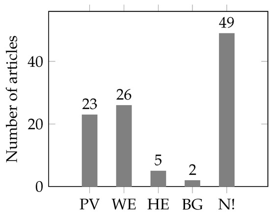
Figure 9.
Results of the literature review for considered renewables (PV: photovoltaic, WE: wind energy, HE: hydro energy, BG: bio gas, N!: not considered).
In [18], stochastic wind energy generation in a IEEE 30-bus grid with two wind parks is considered. The wind energy generation is modeled according to a Weibull distribution. The parameters of the Weibull distribution are calculated using the mayfly algorithm and aquila optimizer. Based on the resulting probability distribution function, an OPF problem with multiple objectives like minimizing emissions of thermal generators or power losses in transmission lines and total operation costs is formulated. The costs for wind energy are divided for over- and underestimating the actual wind energy generation. The OPF problem is solved by the mayfly algorithm. As a result, fluctuating wind energy generation is incorporated by means of according control of thermal generators.
In [41], the authors consider optimal placement and sizing of PV in IEEE 13- and 37-bus systems. For the PV generation, a given load profile is used. The objective of the OPF formulation is to minimize voltage deviation and maximize the PV penetration. The authors use different metaheuristics like artificial bee colony, particle swarm optimization, or differential evolution to solve the OPF problem. As a result, renewable generation of PV is incorporated by means of optimal placement of PV in the grid.
In [37], stochastic wind and PV generation in an IEEE 69-bus grid are considered. Furthermore, a diesel generator and a micro turbine are included in the grid. Wind is modeled according to a Weibull distribution, and solar generation is modeled using a normal probability density function. The objective of the OPF problem is to minimize generation costs, power losses in transmission lines, and voltage deviation. The authors do not describe closer how the costs for PV and wind production are calculated. The locations of PV and wind turbines in the grid are fixed. Fire hawk optimization is used to solve the OPF problem. Wind and PV production are thus incorporated by adapting other controllable loads.
4.7. Considered Grids and Voltage Levels
Most of the reviewed articles do not consider real, existing grids but rather test grids, like IEEE xxx-bus (where xxx denotes the number of buses, there are many different test grids with different numbers of buses). Many articles also consider multiple such test grids with varying numbers of nodes to show scalability of their considered metaheuristic. Also, most articles do not explicitly mention the voltage level. However, those test grids are mostly used to simulate high-voltage grids. Only very few papers consider, for example, real micro grids.
One example for an article with a micro grid is [27]: the authors consider a micro grid consisting of eight nodes. However, there is no further information on the voltage level. Here, it is assumed this is a low-voltage grid. There is also no information on whether this is a real existing grid; the authors call it a “generalizable [micro grid]”.
In [29], the authors consider a hybrid AC-DC radial distribution grid based on an IEEE 30-bus test grid.
Ref. [33] considers a real existing micro grid at Wroclaw University in Poland. The micro grid consists of five nodes; however, the authors do not explicitly mention the voltage level, but it is assumed that it is a low-voltage grid.
In [46], the authors consider an IEEE 30-bus test grid working at 12.6 kV.
5. Discussion and Conclusions
Most of the reviewed articles focus on an optimal coordination of controllable, thermal generators, given certain inflexible loads. Typical objectives of the OPF problem are minimization of voltage deviation, power losses in transmission lines, or fuel costs. The results of such optimizations are settings for control variables, like generator active power or transformer tap settings, as well as state variables like node voltages or angles. However, almost all OPF formulations in the reviewed literature only consider a single time step problem.
Most of those articles compare the performance of their used metaheuristic solvers to other benchmarks in the literature, thus developing efficient solvers. However, none of the reviewed articles research the effect of hyper parameter tuning on the performance of the metaheuristic solver. Often, there are only fixed values given for hyper parameters, but not how those values were determined. In fact, only three papers stated that “optimal” values for hyper parameters were determined by trial and error. And only one article examines the effects of different constraint handling techniques on the performance of the metaheuristic solver.
A few of the reviewed articles also included fluctuating production of renewables like PV, wind energy, or hydro energy in their OPF formulations. The stochastic character of renewable production is incorporated by using according probability density functions. However, all articles consider either optimal placement of newly to-be-installed renewables, subject to typical objectives like minimizing operational costs or effects on grid operation or integration of renewables by means of shifting thermal generation accordingly. None of the reviewed articles consider how to include existing plants into operation of existing low-voltage distribution grids.
Regarding the considered grid for optimization, almost all of the reviewed articles exclusively focus on test grids like IEEE xxx-bus (where xxx stands for a concrete number of buses). These are not real existing grids but are mostly used to evaluate the performance of algorithms used for solving OPF problems. Only two of the reviewed articles examine a real existing grid. Regarding the voltage level of the considered grids, there is no clear indication to be found. This is because it is customary to specify the voltages in p.u. However, due to the structure (multiple branches, partly meshed) of the test grids, it is assumed that those grids are operated in high to middle-voltage. It is therefore also not clear whether the optimization techniques used in the articles reviewed can be directly transferred to low-voltage grids.
Also, almost none of the reviewed articles consider controllable loads in low-voltage distribution grids. Few articles consider electric vehicles, however almost exclusively as static loads added on top of residential load profiles. Only one article considers electric vehicles as real controllable loads—by including charging power as decision variables in the OPF formulation. Also, one article considers aluminium plants as controllable loads by means of adapting their power factor. Only a few other articles consider flexible AC transmission system (FACTS) devices, which might be considered as “controllable loads”. However, loads like electric vehicles or electric heat pumps—with associated requirements like departure time or SOC or heat demands to be covered—were never considered. There exists literature like [100,101,102] that examine optimal coordination of controllable loads; however, such articles do not consider the grid load.
For an optimal scheduling of controllable electric loads in low-voltage distribution grids, accordingly extended OPF formulations must be investigated. These formulations should include requirements associated with controllable loads: for example, desired departure time and SOC for charging electric vehicles or heat demands that need to be covered by electric heat pumps, but also fluctuating production of local renewable generation like PV should be incorporated in such formulations. To allow a meaningful coordination of controllable loads, the optimization problem also has to cover multiple time steps. Thus, additional decision variables and constraints have to be added to the optimization problem. For example, constraints to ensure power balance for all time steps calculate SOCs of EVs or operating limits of other state variables and grid infrastructure.
However, such expanded OPF formulations also require more time for potential solvers to converge to a solution. This is especially true for formulations that involve integer or binary variables. A possible solution can be the usage of metaheuristic solvers—as is already the current state of research. However, only a few articles research the effect of different constraint handling techniques or hyper parameter settings on the performance of the metaheuristic solver. Also, there are no efforts in finding an automated way to determine optimal hyper parameter settings.
Put all together, directions for future research could include:
- whether the reviewed optimization techniques (which were almost always applied in high to middle-voltage grids) can also be applied in low-voltage grids as they are,
- extended OPF formulations (with according constraints) that also account for controllable loads and consider multiple time steps,
- statistical evaluation of the performance of metaheuristic solvers for different constraint handling techniques and settings of hyper parameters, and
- research on automated—e.g., based on machine learning—methods to determine optimal hyper parameters that maximize the performance of the metaheuristic solver.
Covering those research gaps might help to achieve an optimal coordination of multiple controllable loads in low-voltage distribution grids—in a manner so that all requirements of those loads are considered and also a safe operation of the grid is ensured.
Author Contributions
Conceptualization, A.U.; methodology, A.U.; formal analysis, A.U.; investigation, A.U.; resources, I.S. and E.W.; writing—original draft preparation, A.U.; writing—review and editing, I.S., E.W. and A.U.; visualization, A.U.; supervision, I.S. and E.W.; project administration, I.S., E.W. and A.U.; funding acquisition, I.S., E.W. and A.U. All authors have read and agreed to the published version of the manuscript.
Funding
ECS4DRES is supported by the Chips Joint Undertaking under grant agreement number 101139790 and its members, including the top-up funding by Germany, Italy, Slovakia, Spain, and The Netherlands.
Institutional Review Board Statement
Not applicable.
Informed Consent Statement
Not applicable.
Data Availability Statement
Not applicable.
Conflicts of Interest
The authors declare no conflicts of interest.
Abbreviations
The following abbreviations are used in this manuscript:
| EV | Electric Vehicle |
| OPF | Optimal Power Flow |
| CHT | Constraint Handling Technique |
References
- Ulrich, A.; Baum, S.; Stadler, I.; Hotz, C.; Waffenschmidt, E. Maximising Distribution Grid Utilisation by Optimising E-Car Charging Using Smart Meter Gateway Data. Energies 2023, 16, 3790. [Google Scholar] [CrossRef]
- Bartmeyer, P.M.; Lyra, C. A new quadratic relaxation for binary variables applied to the distance geometry problem. Struct. Multidiscip. Optim. 2020, 62, 2197–2201. [Google Scholar] [CrossRef]
- Yuan, G.; Ghanem, B. Binary Optimization via Mathematical Programming with Equilibrium Constraints. Available online: http://arxiv.org/abs/1608.04425 (accessed on 7 November 2023).
- Halim, A.H.; Ismail, I.; Das, S. Performance assessment of the metaheuristic optimization algorithms: An exhaustive review. Artif. Intell. Rev. 2021, 54, 2323–2409. [Google Scholar] [CrossRef]
- Lagaros, N.D.; Kournoutos, M.; Kallioras, N.A.; Nordas, A.N. Constraint handling techniques for metaheuristics: A state-of-the-art review and new variants. Optim. Eng. 2023, 24, 2251–2298. [Google Scholar] [CrossRef]
- Mezura-Montes, E.; Coello Coello, C.A. Constraint-handling in nature-inspired numerical optimization: Past, present and future. Swarm Evol. Comput. 2011, 1, 173–194. [Google Scholar] [CrossRef]
- Hussain, K.; Mohd Salleh, M.N.; Cheng, S.; Shi, Y. Metaheuristic research: A comprehensive survey. Artif. Intell. Rev. 2019, 52, 2191–2233. [Google Scholar] [CrossRef]
- Maurice Farag, M.; Alhamad, R.; Nassif, A.B. Metaheuristic Algorithms in Optimal Power Flow Analysis: A Qualitative Systematic Review. Int. J. Artif. Intell. Tools 2023, 32, 2350032. [Google Scholar] [CrossRef]
- Frank, S.; Steponavice, I.; Rebennack, S. Optimal power flow: A bibliographic survey I. Energy Syst. 2012, 3, 221–258. [Google Scholar] [CrossRef]
- Frank, S.; Rebennack, S. A Primer on Optimal Power Flow: Theory, Formulation and Practical Examples. Colorado School of Mines. 2012. Available online: http://econbus-papers.mines.edu/working-papers/wp201214.pdf (accessed on 13 January 2025).
- Selim, A.; Kamel, S.; Jurado, F. Efficient optimization technique for multiple DG allocation in distribution networks. Appl. Soft Comput. 2020, 86, 105938. [Google Scholar] [CrossRef]
- Boyd, S.P.; Vandenberghe, L. Convex Optimization, 29th ed.; Cambridge University Press: Cambridge, UK, 2023. [Google Scholar]
- Raj, S.; Bhattacharyya, B. Reactive power planning by opposition-based grey wolf optimization method. Int. Trans. Electr. Energy Syst. 2018, 28, e2551. [Google Scholar] [CrossRef]
- Verma, S.; Mukherjee, V. Firefly algorithm for congestion management in deregulated environment. Eng. Sci. Technol. Int. J. 2016, 19, 1254–1265. [Google Scholar] [CrossRef]
- Kennedy, J.; Eberhart, R. Particle swarm optimization. In Proceedings of the International Conference on Neural Networks (ICNN’95), Perth, WA, Australia, 27 November–1 December 1995; Volume 4, pp. 1942–1948. [Google Scholar] [CrossRef]
- Deb, K. An efficient constraint handling method for genetic algorithms. Comput. Methods Appl. Mech. Eng. 2000, 186, 311–338. [Google Scholar] [CrossRef]
- Jamal, R.; Men, B.; Khan, N.H. A Novel Nature Inspired Meta-Heuristic Optimization Approach of GWO Optimizer for Optimal Reactive Power Dispatch Problems. IEEE Access 2020, 8, 202596–202610. [Google Scholar] [CrossRef]
- Khamees, A.K.; Abdelaziz, A.Y.; Eskaros, M.R.; Alhelou, H.H.; Attia, M.A. Stochastic Modeling for Wind Energy and Multi-Objective Optimal Power Flow by Novel Meta-Heuristic Method. IEEE Access 2021, 9, 158353–158366. [Google Scholar] [CrossRef]
- Khan, I.U.; Javaid, N.; Gamage, K.A.A.; Taylor, C.J.; Baig, S.; Ma, X. Heuristic Algorithm Based Optimal Power Flow Model Incorporating Stochastic Renewable Energy Sources. IEEE Access 2020, 8, 148622–148643. [Google Scholar] [CrossRef]
- Birogul, S. Hybrid Harris Hawk Optimization Based on Differential Evolution (HHODE) Algorithm for Optimal Power Flow Problem. IEEE Access 2019, 7, 184468–184488. [Google Scholar] [CrossRef]
- Reddy, A.K.V.K.; Narayana, K.V.L. Symbiotic Learning Grey Wolf Optimizer for Engineering and Power Flow Optimization Problems. IEEE Access 2022, 10, 95229–95280. [Google Scholar] [CrossRef]
- Duman, S. A Modified Moth Swarm Algorithm Based on an Arithmetic Crossover for Constrained Optimization and Optimal Power Flow Problems. IEEE Access 2018, 6, 45394–45416. [Google Scholar] [CrossRef]
- Khan, N.H.; Wang, Y.; Tian, D.; Jamal, R.; Kamel, S.; Ebeed, M. Optimal Siting and Sizing of SSSC Using Modified Salp Swarm Algorithm Considering Optimal Reactive Power Dispatch Problem. IEEE Access 2021, 9, 49249–49266. [Google Scholar] [CrossRef]
- Paul, K.; Sinha, P.; Bouteraa, Y.; Skruch, P.; Mobayen, S. A Novel Improved Manta Ray Foraging Optimization Approach for Mitigating Power System Congestion in Transmission Network. IEEE Access 2023, 11, 10288–10307. [Google Scholar] [CrossRef]
- Huy, T.H.B.; Vo, D.N.; Truong, K.H.; Van Tran, T. Optimal Distributed Generation Placement in Radial Distribution Networks Using Enhanced Search Group Algorithm. IEEE Access 2023, 11, 103288–103305. [Google Scholar] [CrossRef]
- Das, T.; Roy, R.; Mandal, K.K. Impact of the Penetration of Distributed Generation on Optimal Reactive Power Dispatch. Prot. Control. Mod. Power Syst. 2020, 5, 1–26. [Google Scholar] [CrossRef]
- Rousis, A.O.; Konstantelos, I.; Strbac, G. A Planning Model for a Hybrid AC–DC Microgrid Using a Novel GA/AC OPF Algorithm. IEEE Trans. Power Syst. 2020, 35, 227–237. [Google Scholar] [CrossRef]
- Reddy, A.K.V.K.; Narayana, K.V.L. Investigation of a Multi-Strategy Ensemble Social Group Optimization Algorithm for the Optimization of Energy Management in Electric Vehicles. IEEE Access 2024, 10, 12084–12124. [Google Scholar] [CrossRef]
- Ibrahim, M.M.; Hasanien, H.M.; Farag, H.E.Z.; Omran, W.A. Energy Management of Multi-Area Islanded Hybrid Microgrids: A Stochastic Approach. IEEE Access 2023, 11, 101409–101424. [Google Scholar] [CrossRef]
- Kamel, S.; Khasanov, M.; Jurado, F.; Kurbanov, A.; Zawbaa, H.M.; Alathbah, M.A. Simultaneously Distributed Generation Allocation and Network Reconfiguration in Distribution Network Considering Different Loading Levels. IEEE Access 2023, 11, 105916–105934. [Google Scholar] [CrossRef]
- Naguib, M.; Omran, W.A.; Talaat, H.E.A. Performance Enhancement of Distribution Systems via Distribution Network Reconfiguration and Distributed Generator Allocation Considering Uncertain Environment. J. Mod. Power Syst. Clean Energy 2022, 10, 647–655. [Google Scholar] [CrossRef]
- Deb, S.; Houssein, E.H.; Said, M.; Abdelminaam, D.S. Performance of Turbulent Flow of Water Optimization on Economic Load Dispatch Problem. IEEE Access 2021, 9, 77882–77893. [Google Scholar] [CrossRef]
- Suresh, V.; Janik, P.; Guerrero, J.M.; Leonowicz, Z.; Sikorski, T. Microgrid Energy Management System with Embedded Deep Learning Forecaster and Combined Optimizer. IEEE Access 2020, 8, 202225–202239. [Google Scholar] [CrossRef]
- Biswas, P.P.; Suganthan, P.N.; Mallipeddi, R.; Amaratunga, G.A.J. Optimal power flow solutions using differential evolution algorithm integrated with effective constraint handling techniques. Eng. Appl. Artif. Intell. 2018, 68, 81–100. [Google Scholar] [CrossRef]
- Mohamed, A.A.A.; Mohamed, Y.S.; El-Gaafary, A.A.M.; Hemeida, A.M. Optimal power flow using moth swarm algorithm. Electr. Power Syst. Res. 2017, 142, 190–206. [Google Scholar] [CrossRef]
- Le, T.M.C.; Le, X.C.; Huynh, N.N.P.; Doan, A.T.; Dinh, T.V.; Duong, M.Q. Optimal power flow solutions to power systems with wind energy using a highly effective meta-heuristic algorithm. Int. J. Renew. Energy Dev. 2023, 12, 467–477. [Google Scholar] [CrossRef]
- Abed, W.N.A.D. Solving probabilistic optimal power flow with renewable energy sources in distribution networks using fire hawk optimizer. e-Prime Adv. Electr. Eng. Electron. Energy 2023, 6, 100370. [Google Scholar] [CrossRef]
- Daqaq, F.; Ouassaid, M.; Kamel, S.; Ellaia, R.; El-Naggar, M.F. A novel chaotic flower pollination algorithm for function optimization and constrained optimal power flow considering renewable energy sources. Front. Energy Res. 2022, 10, 941705. [Google Scholar] [CrossRef]
- Al-Kaabi, M.; Dumbrava, V.; Eremia, M. Multi Criteria Frameworks Using New Meta-Heuristic Optimization Techniques for Solving Multi-Objective Optimal Power Flow Problems. Energies 2024, 17, 2209. [Google Scholar] [CrossRef]
- Hien, C.T.; Duong, M.P.; Pham, L.H. Skill optimization algorithm for solving optimal power flow problem. Bull. Electr. Eng. Inform. 2024, 13, 12–19. [Google Scholar] [CrossRef]
- Bai, W.; Zhang, W.; Allmendinger, R.; Enyekwe, I.; Lee, K.Y. A Comparative Study of Optimal PV Allocation in a Distribution Network Using Evolutionary Algorithms. Energies 2024, 17, 511. [Google Scholar] [CrossRef]
- Abderrahmani, A.; Abdelfatah, N.; Brahim, G. Artificial intelligence of optimal real power dispatch with constraints of lines overloading. Int. J. Power Electron. Drive Syst. (IJPEDS) 2023, 14, 1885–1893. [Google Scholar] [CrossRef]
- Manoharan, S.; Gnanambal, K. Individual Incremental loading factor based maximum loadability limit prediction using modern optimization tools. J. Eng. Res. 2021, 11, 84–99. [Google Scholar] [CrossRef]
- Zellagui, M.; Belbachir, N.; El-Sehiemy, R.A. Solving the Optimal Power Flow Problem in Power Systems Using the Mountain Gazelle Algorithm. Eng. Proc. 2023, 56, 176. [Google Scholar] [CrossRef]
- Khunkitti, S.; Premrudeepreechacharn, S.; Siritaratiwat, A. A Two-Archive Harris Hawk Optimization for Solving Many-Objective Optimal Power Flow Problems. IEEE Access 2023, 11, 134557–134574. [Google Scholar] [CrossRef]
- Raza, A.; Zahid, M.; Chen, J.; Qaisar, S.M.; Ilahi, T.; Waqar, A.; Alzahrani, A. A Novel Integration Technique for Optimal Location & Sizing of DG Units with Reconfiguration in Radial Distribution Networks Considering Reliability. IEEE Access 2023, 11, 123610–123624. [Google Scholar] [CrossRef]
- Hassan, M.H.; Kamel, S.; Domínguez-García, J.L.; Molu, R.J.J. Integrating renewable energy and V2G uncertainty into optimal power flow: A gradient bald eagle search optimization algorithm with local escaping operator. IET Renew. Power Gener. 2023, 18, 4119–4152. [Google Scholar] [CrossRef]
- Aurangzeb, K.; Shafiq, S.; Alhussein, M.; Pamir; Javaid, N.; Imran, M. An effective solution to the optimal power flow problem using meta-heuristic algorithms. Front. Energy Res. 2023, 11, 1170570. [Google Scholar] [CrossRef]
- Zadehbagheri, M.; Ildarabadi, R.; Javadian, A.M. Optimal Power Flow in the Presence of HVDC Lines Along with Optimal Placement of FACTS in Order to Power System Stability Improvement in Different Conditions: Technical and Economic Approach. IEEE Access 2023, 11, 57745–57771. [Google Scholar] [CrossRef]
- Warid, W.; Hizam, H.; Mariun, N.; Abdul-Wahab, N.I. Optimal Power Flow Using the Jaya Algorithm. Energies 2016, 9, 678. [Google Scholar] [CrossRef]
- Tamilselvan, V.; Jayabarathi, T.; Raghunathan, T.; Yang, X.S. Optimal capacitor placement in radial distribution systems using flower pollination algorithm. Alex. Eng. J. 2018, 57, 2775–2786. [Google Scholar] [CrossRef]
- Ullah, Z.; Wang, S.; Radosavljevic, J.; Lai, J. A Solution to the Optimal Power Flow Problem Considering WT and PV Generation. IEEE Access 2019, 7, 46763–46772. [Google Scholar] [CrossRef]
- Ali, M.H.; Kamel, S.; Hassan, M.H.; Tostado-Véliz, M.; Zawbaa, H.M. An improved wild horse optimization algorithm for reliability based optimal DG planning of radial distribution networks. Energy Rep. 2022, 8, 582–604. [Google Scholar] [CrossRef]
- Hussain, K.; Zhu, W.; Mohd Salleh, M.N. Long-Term Memory Harris’ Hawk Optimization for High Dimensional and Optimal Power Flow Problems. IEEE Access 2019, 7, 147596–147616. [Google Scholar] [CrossRef]
- Duong, T.L.; Duong, M.Q.; Phan, V.D.; Nguyen, T.T. Optimal Reactive Power Flow for Large-Scale Power Systems Using an Effective Metaheuristic Algorithm. J. Electr. Comput. Eng. 2020, 2020, 6382507. [Google Scholar] [CrossRef]
- Rawa, M.; Abusorrah, A.; Bassi, H.; Mekhilef, S.; Ali, Z.M.; Abdel Aleem, S.H.E.; Hasanien, H.M.; Omar, A.I. Economical-technical-environmental operation of power networks with wind-solar-hydropower generation using analytic hierarchy process and improved grey wolf algorithm. Ain Shams Eng. J. 2021, 12, 2717–2734. [Google Scholar] [CrossRef]
- Nadeem, M.; Imran, K.; Khattak, A.; Ulasyar, A.; Pal, A.; Zeb, M.Z.; Khan, A.N.; Padhee, M. Optimal Placement, Sizing and Coordination of FACTS Devices in Transmission Network Using Whale Optimization Algorithm. Energies 2020, 13, 753. [Google Scholar] [CrossRef]
- Abdo, M.; Kamel, S.; Ebeed, M.; Yu, J.; Jurado, F. Solving Non-Smooth Optimal Power Flow Problems Using a Developed Grey Wolf Optimizer. Energies 2018, 11, 1692. [Google Scholar] [CrossRef]
- Chintam, J.R.; Daniel, M. Real-Power Rescheduling of Generators for Congestion Management Using a Novel Satin Bowerbird Optimization Algorithm. Energies 2018, 11, 183. [Google Scholar] [CrossRef]
- Oda, E.S.; Abdelsalam, A.A.; Abdel-Wahab, M.N.; El-Saadawi, M.M. Distributed generations planning using flower pollination algorithm for enhancing distribution system voltage stability. Ain Shams Eng. J. 2017, 8, 593–603. [Google Scholar] [CrossRef]
- Khan, A.; Hizam, H.; Wahab, N.I.b.A.; Othman, M.L. Optimal power flow using hybrid firefly and particle swarm optimization algorithm. PLoS ONE 2020, 15, e0235668. [Google Scholar] [CrossRef]
- Trivedi, I.N.; Jangir, P.; Parmar, S.A. Optimal power flow with enhancement of voltage stability and reduction of power loss using ant-lion optimizer. Cogent Eng. 2016, 3, 1208942. [Google Scholar] [CrossRef]
- Hemeida, M.G.; Alkhalaf, S.; Mohamed, A.A.A.; Ibrahim, A.A.; Senjyu, T. Distributed Generators Optimization Based on Multi-Objective Functions Using Manta Rays Foraging Optimization Algorithm (MRFO). Energies 2020, 13, 3847. [Google Scholar] [CrossRef]
- Abdollahi, A.; Ghadimi, A.A.; Miveh, M.R.; Mohammadi, F.; Jurado, F. Optimal Power Flow Incorporating FACTS Devices and Stochastic Wind Power Generation Using Krill Herd Algorithm. Electronics 2020, 9, 1043. [Google Scholar] [CrossRef]
- Singh, N.K.; Koley, C.; Gope, S.; Dawn, S.; Ustun, T.S. An Economic Risk Analysis in Wind and Pumped Hydro Energy Storage Integrated Power System Using Meta-Heuristic Algorithm. Sustainability 2021, 13, 13542. [Google Scholar] [CrossRef]
- Khamees, A.K.; Abdelaziz, A.Y.; Eskaros, M.R.; El-Shahat, A.; Attia, M.A. Optimal Power Flow Solution of Wind-Integrated Power System Using Novel Metaheuristic Method. Energies 2021, 14, 6117. [Google Scholar] [CrossRef]
- Saha, A.; Bhattacharya, A.; Das, P.; Chakraborty, A.K. A novel approach towards uncertainty modeling in multiobjective optimal power flow with renewable integration. Int. Trans. Electr. Energy Syst. 2019, 29, e12136. [Google Scholar] [CrossRef]
- Mouassa, S.; Althobaiti, A.; Jurado, F.; Ghoneim, S.S.M. Novel Design of Slim Mould Optimizer for the Solution of Optimal Power Flow Problems Incorporating Intermittent Sources: A Case Study of Algerian Electricity Grid. IEEE Access 2022, 10, 22646–22661. [Google Scholar] [CrossRef]
- Li, Z.; Cao, Y.; Dai, L.V.; Yang, X.; Nguyen, T.T. Optimal Power Flow for Transmission Power Networks Using a Novel Metaheuristic Algorithm. Energies 2019, 12, 4310. [Google Scholar] [CrossRef]
- Diab, H.; Abdelsalam, M.; Abdelbary, A. A Multi-Objective Optimal Power Flow Control of Electrical Transmission Networks Using Intelligent Meta-Heuristic Optimization Techniques. Sustainability 2021, 13, 4979. [Google Scholar] [CrossRef]
- Ali, M.H.; El-Rifaie, A.M.; Youssef, A.A.F.; Tulsky, V.N.; Tolba, M.A. Techno-Economic Strategy for the Load Dispatch and Power Flow in Power Grids Using Peafowl Optimization Algorithm. Energies 2023, 16, 846. [Google Scholar] [CrossRef]
- Al-Kaabi, M.; Dumbrava, V.; Eremia, M. Single and Multi-Objective Optimal Power Flow Based on Hunger Games Search with Pareto Concept Optimization. Energies 2022, 15, 8328. [Google Scholar] [CrossRef]
- Dash, S.; Subhashini, K.R.; Satapathy, J. Efficient utilization of power system network through optimal location of FACTS devices using a proposed hybrid meta-heuristic Ant Lion-Moth Flame-Salp Swarm optimization algorithm. Int. Trans. Electr. Energy Syst. 2020, 30, e12402. [Google Scholar] [CrossRef]
- Emam, M.M.; Houssein, E.H.; Tolba, M.A.; Zaky, M.M.; Hamouda Ali, M. Application of modified artificial hummingbird algorithm in optimal power flow and generation capacity in power networks considering renewable energy sources. Sci. Rep. 2023, 13, 21446. [Google Scholar] [CrossRef]
- Alasali, F.; Nusair, K.; Obeidat, A.M.; Foudeh, H.; Holderbaum, W. An analysis of optimal power flow strategies for a power network incorporating stochastic renewable energy resources. Int. Trans. Electr. Energy Syst. 2021, 31, e13060. [Google Scholar] [CrossRef]
- Swief, R.A.; Hassan, N.M.; Hasanien, H.M.; Abdelaziz, A.Y.; Kamh, M.Z. AC&DC optimal power flow incorporating centralized/decentralized multi-region grid control employing the whale algorithm. Ain Shams Eng. J. 2021, 12, 1907–1922. [Google Scholar] [CrossRef]
- Bentouati, B.; Chettih, S.; Chaib, L. Interior search algorithm for optimal power flow with non-smooth cost functions. Cogent Eng. 2017, 4, 1292598. [Google Scholar] [CrossRef]
- Chang, G.W.; Chinh, N.C.; Sinatra, C. Equilibrium Optimizer-Based Approach of PV Generation Planning in a Distribution System for Maximizing Hosting Capacity. IEEE Access 2022, 10, 118108–118122. [Google Scholar] [CrossRef]
- Gupta, S.; Kumar, N.; Srivastava, L.; Malik, H.; Pliego Marugán, A.; García Márquez, F.P. A Hybrid Jaya–Powell’s Pattern Search Algorithm for Multi-Objective Optimal Power Flow Incorporating Distributed Generation. Energies 2021, 14, 2831. [Google Scholar] [CrossRef]
- Home-Ortiz, J.M.; De Oliveira, W.C.; Mantovani, J.R.S. Optimal Power Flow Problem Solution Through a Matheuristic Approach. IEEE Access 2021, 9, 84576–84587. [Google Scholar] [CrossRef]
- Khan, M.W.; Muhammad, Y.; Raja, M.A.Z.; Ullah, F.; Chaudhary, N.I.; He, Y. A New Fractional Particle Swarm Optimization with Entropy Diversity Based Velocity for Reactive Power Planning. Entropy 2020, 22, 1112. [Google Scholar] [CrossRef] [PubMed]
- Üney, M.Ş.; Çetinkaya, N. New Metaheuristic Algorithms for Reactive Power Optimization. Teh. Vjesn. 2019, 26, 1427–1433. [Google Scholar] [CrossRef]
- Suresh, V.; Janik, P.; Jasinski, M. Metaheuristic approach to optimal power flow using mixed integer distributed ant colony optimization. Arch. Electr. Eng. 2020, 69, 335–348. [Google Scholar] [CrossRef]
- Saha, A.; Bhattacharya, A.; Chakraborty, A.K.; Das, P. A Powerful Metaheuristic Algorithm to Solve Static Optimal Power Flow Problems: Symbiotic Organisms Search. Int. J. Electr. Eng. Inform. 2018, 10, 585–614. [Google Scholar] [CrossRef]
- Pandya, S.B.; Visumathi, J.; Mahdal, M.; Mahanta, T.K.; Jangir, P. A Novel MOGNDO Algorithm for Security-Constrained Optimal Power Flow Problems. Electronics 2022, 11, 3825. [Google Scholar] [CrossRef]
- Swaminathan, D.; Rajagopalan, A. Optimized Network Reconfiguration with Integrated Generation Using Tangent Golden Flower Algorithm. Energies 2022, 15, 8158. [Google Scholar] [CrossRef]
- Qin, L.; Xu, T.; Li, S.; Chen, Z.; Zhang, Q.; Tian, J.; Lin, Y. Coot Algorithm for Optimal Carbon–Energy Combined Flow of Power Grid with Aluminum Plants. Front. Energy Res. 2022, 10, 856314. [Google Scholar] [CrossRef]
- Mohamed, A.A.; Kamel, S.; Hassan, M.H.; Zeinoddini-Meymand, H. CAVOA: A chaotic optimization algorithm for optimal power flow with facts devices and stochastic wind power generation. IET Gener. Transm. Distrib. 2024, 18, 121–144. [Google Scholar] [CrossRef]
- Khan, M.S.; Waheed, D.; Shahzad, S.; Afzal, S.; Killic, H. Optimal allocation of distributed generation in meshed power networks: A metaheuristic approach. IET Renew. Power Gener. 2024, 18, 1570–1595. [Google Scholar] [CrossRef]
- Belbachir, N.; Kamel, S.; Hashim, F.A.; Yu, J.; Zeinoddini-Meymand, H.; Sabbeh, S.F. Optimizing the hybrid PVDG and DSTATCOM integration in electrical distribution systems based on a modified homonuclear molecules optimization algorithm. IET Renew. Power Gener. 2023, 17, 3075–3096. [Google Scholar] [CrossRef]
- Wang, D.; Peng, D.; Huang, D.; Ren, L.; Yang, M.; Zhao, H. Research on short-term and mid-long term optimal dispatch of multi-energy complementary power generation system. IET Renew. Power Gener. 2022, 16, 1354–1367. [Google Scholar] [CrossRef]
- Helmi, A.M.; Abo-Elyousr, F.K.; Haes Alhelou, H.; Ramadan, H.S. Dual-stage day-ahead optimized performance of renewable-based microgrids. IET Renew. Power Gener. 2023, 17, 2050–2063. [Google Scholar] [CrossRef]
- Pérez, C.A.P.; Espinosa, L.G.; Fuentefria, A.S. Reduction of energy losses through the integration of photovoltaic power plants in distribution networks. IET Gener. Transm. Distrib. 2023, 17, 3739–3750. [Google Scholar] [CrossRef]
- Mohamed, M.A.E.H.; Kamel, S.; Wulfran, F.M. Metaheuristic-based graded objective function strategy for optimal thyristor-controlled series capacitors estimation in weak distribution systems with uncertain distributed generation. IET Gener. Transm. Distrib. 2024, 18, 1325–1342. [Google Scholar] [CrossRef]
- Bastawy, M.; Ebeed, M.; Ali, A.; Shaaban, M.F.; Khan, B.; Kamel, S. Optimal day-ahead scheduling in micro-grid with renewable based DGs and smart charging station of EVs using an enhanced manta-ray foraging optimisation. IET Renew. Power Gener. 2022, 16, 2413–2428. [Google Scholar] [CrossRef]
- Khasanov, M.; Kamel, S.; Rahmann, C.; Hasanien, H.M.; Al-Durra, A. Optimal distributed generation and battery energy storage units integration in distribution systems considering power generation uncertainty. IET Gener. Transm. Distrib. 2021, 15, 3400–3422. [Google Scholar] [CrossRef]
- Abuelrub, A.; Awwad, B.; Al-Masri, H.M.K. Solving wind-integrated unit commitment problem by a modified African vultures optimization algorithm. IET Gener. Transm. Distrib. 2023, 17, 3678–3691. [Google Scholar] [CrossRef]
- Ramadan, H.S.; Iqbal, M.; Becherif, M.; Haes Alhelou, H. Efficient control and multi-criteria energy scheduling of renewable-based utility grid via pareto-metaheuristic optimizers. IET Renew. Power Gener. 2022, 16, 1246–1266. [Google Scholar] [CrossRef]
- Schlüter, M.; Egea, J.A.; Banga, J.R. Extended ant colony optimization for non-convex mixed integer nonlinear programming. Comput. Oper. Res. 2009, 36, 2217–2229. [Google Scholar] [CrossRef]
- Habib, H.U.R.; Waqar, A.; Junejo, A.K.; Ismail, M.M.; Hossen, M.; Jahangiri, M.; Kabir, A.; Khan, S.; Kim, Y.S. Optimal Planning of Residential Microgrids Based on Multiple Demand Response Programs Using ABC Algorithm. IEEE Access 2022, 10, 116564–116626. [Google Scholar] [CrossRef]
- Lokeshgupta, B.; Sivasubramani, S. Optimal operation of a residential microgrid with demand side management. In Proceedings of the 2019 IEEE PES Innovative Smart Grid Technologies Europe, Bucharest, Romania, 29 September–2 October 2019; pp. 1–5. [Google Scholar] [CrossRef]
- Zanjani, S.M.H.; Shahinzadeh, H.; Pourmirza, Z.; Kabalci, E.; Muyeen, S.M.; Benbouzid, M. Optimal Operation of a Residential Energy Hub in the Presence of an Electric Vehicle using Whale Optimization Algorithm. In Proceedings of the 2022 26th International Electrical Power Distribution Conference (EPDC), Tehran, Iran, 11–12 May 2022; pp. 84–89. [Google Scholar] [CrossRef]

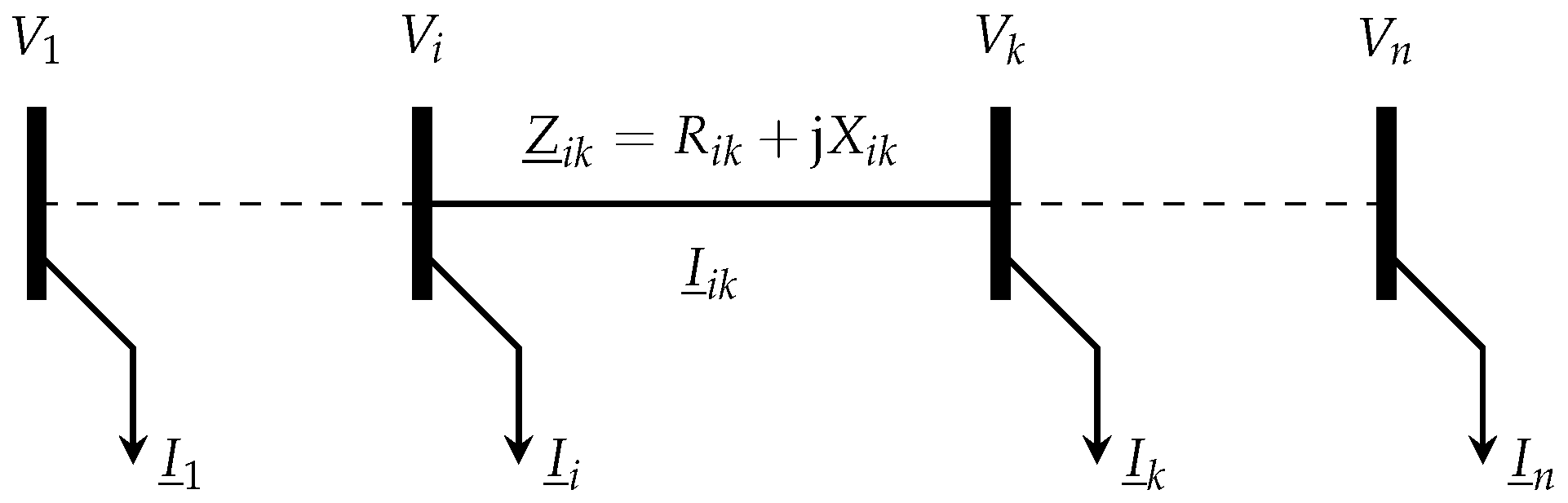

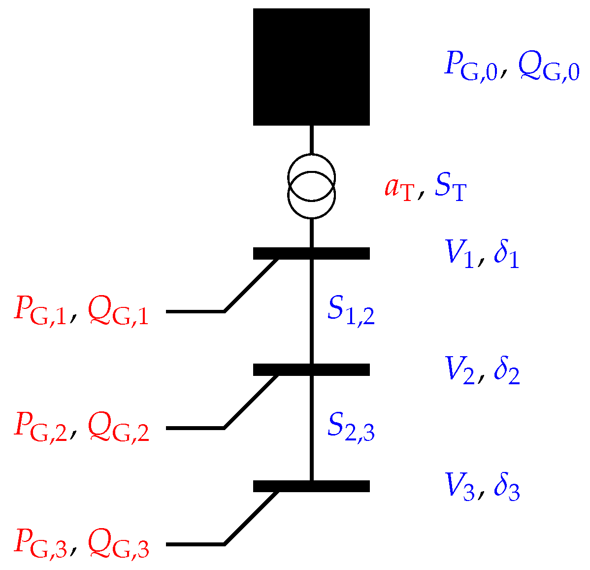
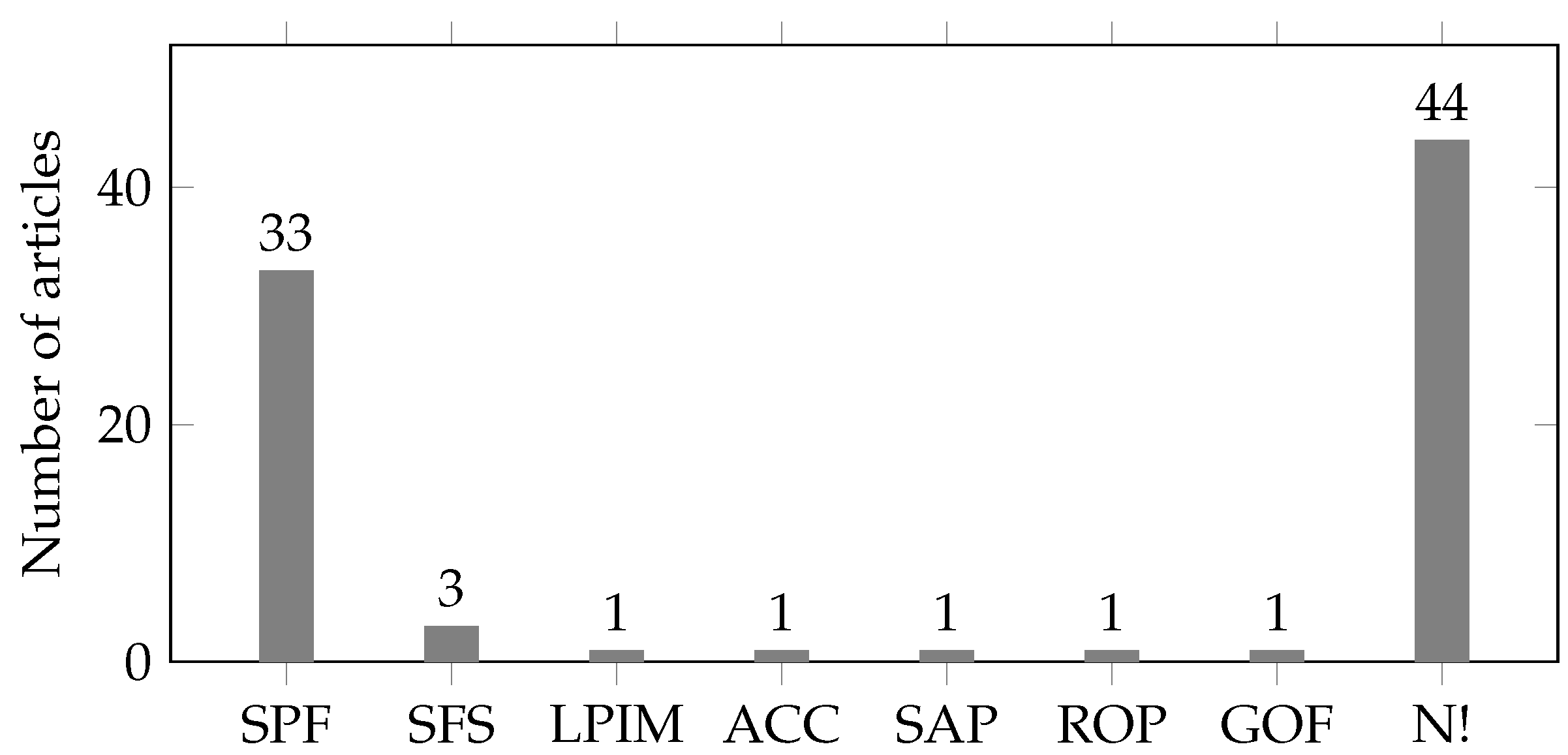
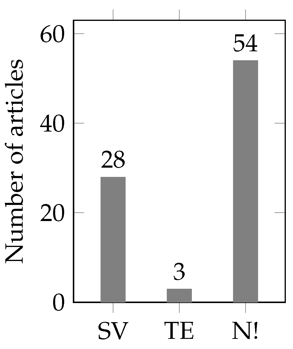
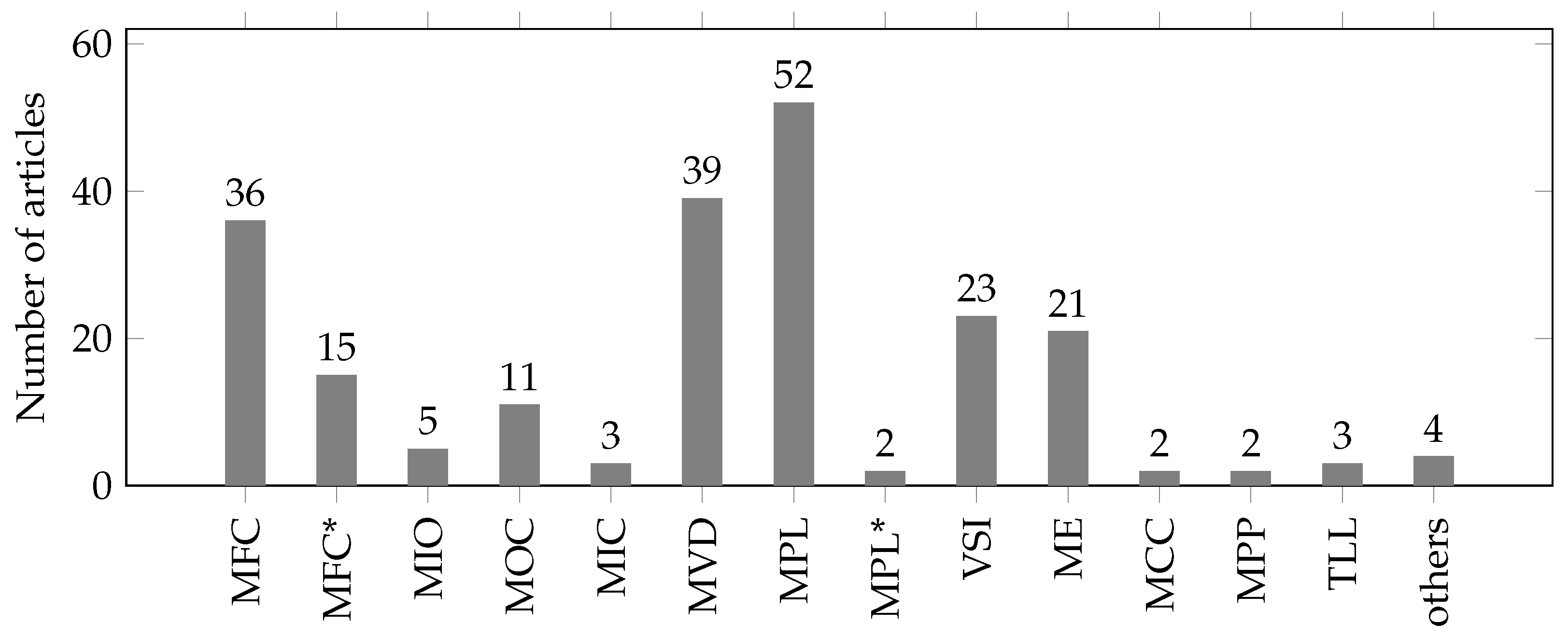
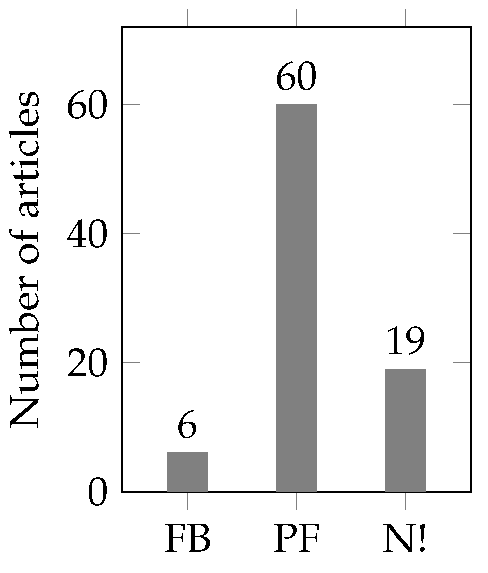
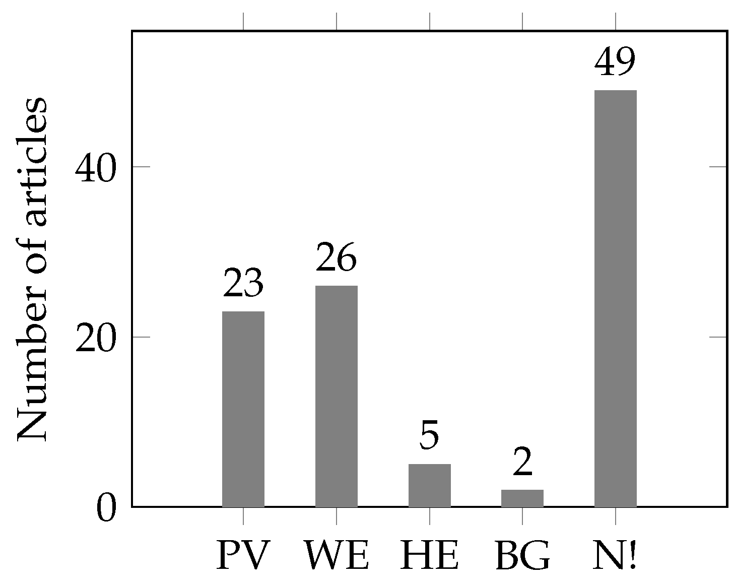
Disclaimer/Publisher’s Note: The statements, opinions and data contained in all publications are solely those of the individual author(s) and contributor(s) and not of MDPI and/or the editor(s). MDPI and/or the editor(s) disclaim responsibility for any injury to people or property resulting from any ideas, methods, instructions or products referred to in the content. |
© 2025 by the authors. Licensee MDPI, Basel, Switzerland. This article is an open access article distributed under the terms and conditions of the Creative Commons Attribution (CC BY) license (https://creativecommons.org/licenses/by/4.0/).