A Practical Short-Circuit Current Calculation Method for Renewable Energy Plants Based on Single-Machine Multiplication

Abstract

In non-synchronous machine sources (N-SMSs), power sources are connected to the grid through power electronic devices, which typically exhibit a voltage-controlled current source characteristic during faults. Due to the current-limiting feature of inverters, the voltage and current demonstrate a strong nonlinearity. As a result, the short-circuit current (SCC) of N-SMSs is commonly calculated using iterative methods. For renewable energy plants, which contain a large number of N-SMSs, the calculation is often based on the single-machine multiplication method, ignoring internal discrepancies among machines. To address these issues, this paper proposes a calculation method for the SCC contributed by a renewable energy plant based on single-machine multiplication. This method is simple, does not require iteration, and ensures engineering practicability. This paper first analyzes the SCC calculation model under a low-voltage ride-through (LVRT) control strategy. Inspired by the single-machine multiplication approach, a fast initial voltage calculation method at the machine terminal is proposed, along with an active current correction method. With this approach, a more accurate SCC can be obtained, avoiding convergence issues and ensuring practical applicability in engineering. The validity of this method is verified through PSCAD/EMTDC simulations. The error in calculating SCC does not exceed 3.02%. Compared with the single-machine multiplication method, the accuracy is significantly improved, while the accuracy is roughly equivalent to that of the iterative method.

1. Introduction

In recent years, with the increasing penetration of renewable energy sources, such as wind and photovoltaic power, into the grid and the rise of flexible AC/DC transmission technologies, power systems have exhibited a “dual-high” development trend characterized by a high proportion of renewable energy and a high penetration of power electronic devices. This shift has resulted in significant changes in the operational characteristics of power systems [1,2,3]. SCC analysis and calculation are fundamental components of system planning, design, and operational analysis [4,5]. Unlike synchronous machines, N-SMSs used in renewable energy systems are typically connected to the grid via power electronic devices, with the control mechanisms being dominated by these devices. As a result, the SCC response is influenced by control strategies and has a limited overcurrent capability.

Research on SCCs in N-SMSs can be divided into single-machine-level and plant-level studies. Current research at the single-machine level mainly focuses on the derivation of analytical expressions for SCCs under different control strategies, as well as the impact of control parameters on transient processes [6,7,8,9]. It also includes the influence of pre-fault conditions, LVRT control strategies, and limiter parameters on steady-state SCCs [10,11]. For example, the work presented in [6] investigated the transient characteristics of fault currents and their influencing factors in both linear and nonlinear regions of the controller. A theoretical method for calculating photovoltaic fault currents, including transient and steady-state models, was proposed in [7], which further explored the impact of control parameters and fault severity on fault characteristics. Analytical expressions for SCCs, considering the activation time of crowbar protection, were derived in [8], with an analysis of how crowbar resistance affects the fault current of doubly-fed wind turbines. Meanwhile, the work presented in [9] derived expressions for SCCs under various fault ride-through modes for single machines. The effects of control strategies on the transient process of wind turbine generators during faults were considered in [10], where single-machine equivalent models for doubly-fed and permanent-magnet wind turbine generators were developed. Furthermore, the work presented in [11] examined the impact of voltage-source converter limiters on SCCs. These studies show that research on single-machine SCCs is relatively mature. Since the converter’s inertia time is very short, the SCC typically stabilizes after a transient period of about 10 ms. In the steady state, N-SMSs can be treated as voltage-controlled current sources, with a nonlinear voltage–current relationship due to the presence of current limiters.

At the plant level, SCC research has mainly focused on the equivalent modeling of renewable energy plants. These plants may contain dozens or even more N-SMSs, and most existing electromechanical transient calculation models for SCCs do not include detailed models of renewable energy plants. Because of the system’s nonlinearity, iterative calculations are required, and the commonly used method is single-machine multiplication. While computationally convenient, this method neglects the differences between generators and the effects of transmission lines, leading to reduced accuracy. Therefore, simplifying the equivalent model of renewable energy plants is a key issue. The single-machine multiplication method was used for the equivalent modeling of renewable energy plants in [12], which was then combined with traditional synchronous machine SCC calculation methods. A local iteration method for fault regions was proposed to avoid the convergence issues encountered with global iteration methods. Current equivalent modeling approaches primarily focus on control strategies [13,14,15] and dynamic characteristics [16,17]. For instance, the work presented in [10] grouped wind turbines by their types and control strategies in a mixed wind farm, equivalently modeling the farm as two turbines. However, this approach overlooked the distribution characteristics of the turbines within the farm. The turbines were categorized into two groups based on the voltage drop and pre-fault active power output, significantly improving accuracy compared with single-machine multiplication. However, errors remained because the iterative method was not used for calculating the voltage at the plant connection point. The work presented in [18] considered the transient response process and established a multi-machine equivalent model for distributed photovoltaic systems based on the concept of homogeneous equivalence. The work presented in [19] proposed a multistage hierarchical parameter identification process, utilizing data from phasor measurement units, to develop a dynamic equivalent model for wind farms and describe their dynamic behavior during system disturbances. The work presented in [20] identified the clustering index based on the clustering characteristics of the active power transient response curve under the LVRT strategy and performed clustering equivalence for wind turbines in the wind farm, with the acquisition of the clustering algorithm or index requiring computational assistance due to its complexity. Additionally, the work presented in [21] introduced a clustering method for photovoltaic power plants based on the operation of a fault current-limiting loop, establishing a SCC calculation model using a multi-machine representation. However, the voltage dip values used for clustering required a complex iterative solution. Lastly, the work presented in ref. [22] presented an SCC calculation method that accounted for the internal topology of renewable energy plants, offering accurate results by solving a system of linear equations under the assumption of only reactive current. However, it neglected the effect of an active current, leading to potential errors.

In summary, there are two main challenges in calculating the SCC contributed by a renewable energy plant. The first is that the port voltage and current are nonlinear, necessitating iterative calculations. The second is the presence of numerous N-SMSs within the plant, leading to convergence issues and excessive computational resource consumption during iterative calculations. To address these challenges, this paper presents a practical method for calculating the SCC of a renewable energy plant. This method accurately determines the SCC provided by the station under a reactive power priority fault ride-through strategy. The calculation error is significantly improved compared with the single-machine multiplication method, and it does not require iterative computation. Additionally, the algorithm’s time complexity is not increased, and there is no issue with the initial value affecting convergence.

The structure of this paper is as follows:

Section 1 introduces the typical control strategies of the full-power converter, including the voltage–current double-closed-loop control strategy in steady-state operation and the reactive power priority control strategy during faults. Based on this, the expressions for the terminal voltage and current of the N-SMSs are derived.

Section 2 presents a calculation method for the SCC of a renewable energy plant, which is divided into two steps. The first step involves calculating the initial voltage at the source port of each N-SMS using the single-machine multiplication, considering only the reactive current. The second step corrects the port voltage based on the initial value, accounting for the effect of the active current. Finally, the short-circuit current is determined using the corrected port voltage.

Section 3 presents the simulation verification of the proposed theory. In this section, a chain-structured permanent-magnet direct-drive wind farm is modeled in PSCAD, and the control strategy outlined in Section 1 is applied. The simulation results in Section 4 confirm the feasibility of the proposed method.

Section 5 summarizes the paper and discusses the advantages and limitations of the proposed method, along with key directions for future work.

2. The Typical Operating Control Strategies of N-SMSs

N-SMSs are connected to the grid through power electronic devices and can be classified based on their level of grid isolation. Full-power inverter-based sources, represented by photovoltaic systems and permanent-magnet direct-drive wind turbines, and partial-power inverter-based sources, represented by doubly fed induction generators, are the two main categories. Based on grid connection control strategies, they can be divided into grid-following (GFL) and grid-forming (GFM) types. Similar to synchronous machines, they can also be classified according to node types, such as PV, PQ, and Vθ connections. Since the SCC of N-SMSs is related to the control strategy during faults, this paper introduces the grid-following control strategy of full-power inverter-based sources as an example. The grid-connected inverter and its control system are shown in Figure 1, which will be described in detail below.

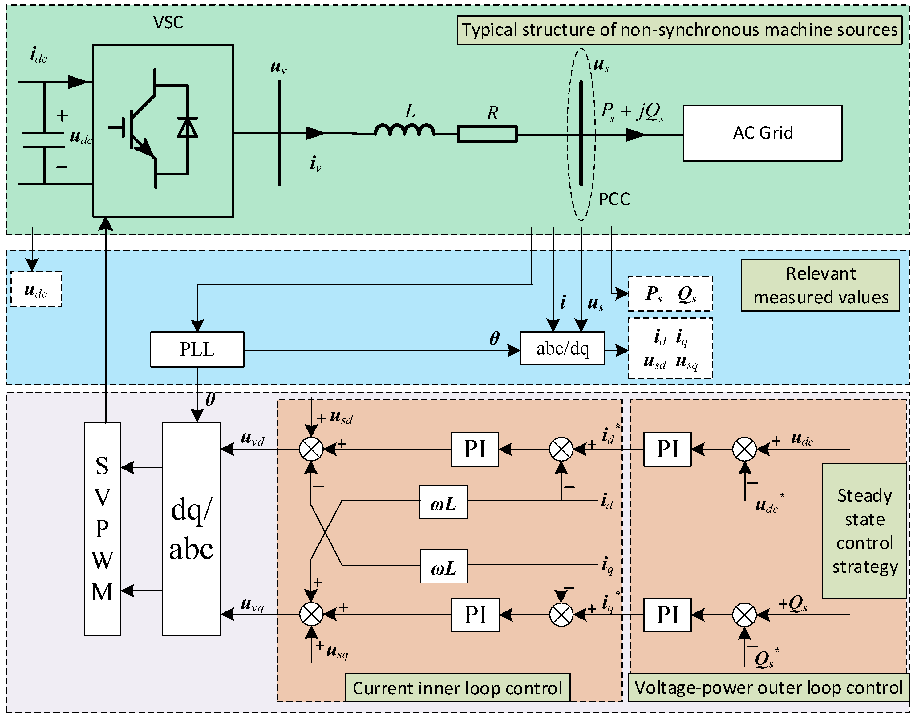
2.1. Full-Power Inverter-Based Power Source Control Strategy

In the synchronously rotating reference frame, the voltage and current equations of the grid-side inverter are given by

$$\left\{\begin{array}{l}{u}_{\mathrm{d}}=L{\displaystyle \frac{d{i}_{\mathrm{d}}}{dt}}+R{i}_{\mathrm{d}}-\omega L{i}_{\mathrm{q}}+u_{\mathrm{gd}}\hfill \\ u_{\mathrm{q}}=L{\displaystyle \frac{d{i}_{\mathrm{q}}}{dt}}+R{i}_{\mathrm{q}}+\omega L{i}_{\mathrm{d}}+u_{\mathrm{gq}}\hfill \end{array}\right.$$

(1)

where

• u_d and u_q are the d- and q-axis components of the inverter bridge output voltage.
• i_d and i_q are the d- and q-axis components of the inverter output current.
• u_gd and u_gq are the d- and q-axis components of the grid voltage at the connection point.
• L and R are the inductance and resistance of the AC-side filter.
• ω is the synchronous angular velocity.

Grid-following inverters use a phase-locked loop to track the grid voltage and present either a “current source” or “power source” characteristic. Typically, grid voltage-oriented vector control is applied, i.e., u_gd = U_g and u_gq = 0. In this case, the output power of the inverter is

$$\left\{\begin{array}{l}P={\displaystyle \frac{3}{2}}(u_{\mathrm{gd}}{i}_{\mathrm{d}}+u_{\mathrm{gq}}{i}_{\mathrm{q}})={\displaystyle \frac{3}{2}}{U}_{\mathrm{g}}{i}_{\mathrm{d}}\hfill \\ Q={\displaystyle \frac{3}{2}}(u_{\mathrm{gq}}{i}_{\mathrm{d}}-u_{\mathrm{gd}}{i}_{\mathrm{q}})=-{\displaystyle \frac{3}{2}}{U}_{\mathrm{g}}{i}_{\mathrm{q}}\hfill \end{array}\right.$$

(2)

where

• P and Q represent the real and reactive power output of the inverter, respectively.
• U_g is the grid-side voltage at the connection point.

From Equation (2), it can be seen that the active and reactive power output of the inverter are linearly related to i_d and i_q, respectively. This means that decoupled control of P and Q can be achieved by controlling i_d and i_q. Since the output power of photovoltaic and wind systems depends on environmental factors, such as sunlight and wind speed, the real power P is typically not given directly. Instead, it is determined by the maximum power point tracking control of the inverter at the machine side. The variation in the active power is reflected in the DC link voltage of the grid-side inverter. Therefore, the active power control variable for the grid-side inverter is the DC link voltage.

Under normal conditions, the inverter operates at unity power factor, using a voltage–current dual-loop control. Due to the excellent characteristics of the PI controller, PI control is commonly used, and its control equation is

$$\left\{\begin{array}{l}{i}_{\mathrm{d}}^{*}=k_{\mathrm{vP}}(u_{\mathrm{dc}}^{*}-u_{\mathrm{dc}})+k_{\mathrm{vI}}{\displaystyle \int (u_{\mathrm{dc}}^{*}-u_{\mathrm{dc}})}dt\\ i_{\mathrm{q}}^{*}=k_{\mathrm{vP}}(Q_{\mathrm{s}}^{*}-Q_{\mathrm{s}})+k_{\mathrm{vI}}{\displaystyle \int (Q_{\mathrm{s}}^{*}-Q_{\mathrm{s}})}dt\\ u_{\mathrm{vd}}=k_{\mathrm{P}}(i_{\mathrm{d}}^{*}-i_{\mathrm{d}})+k_{\mathrm{I}}{\displaystyle \int (i_{\mathrm{d}}^{*}-i_{\mathrm{d}})}dt-\omega L{i}_{\mathrm{q}}+u_{\mathrm{gd}}\\ u_{\mathrm{vd}}=k_{\mathrm{P}}(i_{\mathrm{q}}^{*}-i_{\mathrm{q}})+k_{\mathrm{I}}{\displaystyle \int (i_{\mathrm{q}}^{*}-i_{\mathrm{q}})}dt+\omega L{i}_{\mathrm{d}}+u_{\mathrm{gq}}\end{array}\right.$$

(3)

where

• The superscript * represents the controller’s reference value.
• u_dc is the DC link voltage of the inverter.
• Q_s is the reactive power.
• k_vP and k_vI are the proportional and integral parameters of the voltage outer-loop controller, respectively.
• u_vd and u_vq are the d- and q-axis components of the inverter bridge output voltage.
• k_P and k_I are the proportional and integral parameters of the current inner-loop controller, respectively.

2.2. SCC and Voltage Relationship Under Low-Voltage Ride-Through Control Strategy

When a short-circuit fault occurs in the grid, the terminal voltage of the N-SMSs drops, requiring the generator to provide reactive power to support the grid voltage. During this period, the voltage control outer loop is disabled, and the reference value for the current inner loop is determined by the low-voltage ride-through (LVRT) control strategy.

Taking a wind farm as an example, according to grid connection standards [23], when the voltage at the connection point drops to 20% of the nominal voltage, the wind turbine should remain connected to the grid. During symmetrical faults, the requirement for reactive current during the low-voltage ride-through period is given by:

$$\begin{array}{cc}\Delta I_{\mathrm{t}}=K_1\times (0.9-U_{\mathrm{t}})\times I_{\mathrm{N}}& 0.2\le U_{\mathrm{t}}\le 0.9\end{array}$$

(4)

where

• ΔI_t is the dynamic reactive current increment injected by the wind farm.
• K₁ is the proportional coefficient for dynamic reactive current in the wind farm, with a recommended range of no less than 1.5 and preferably no greater than 3.
• U_t is the per-unit voltage at the wind farm grid connection point.
• I_N is the rated current of the wind farm.

Since the reactive power command for the wind turbine is zero in the steady state, I_q^∗ = ΔI_t. From Equation (4), it can be observed that as K₁ increases and U_t decreases, I_q^∗ increases, causing the limiter to saturate more easily. When saturation occurs, I_q^∗ becomes the saturation limit value I_max. Therefore, the voltage constraint at critical saturation can be derived as

$$K_1(0.9-U_{1\mathrm{e}})I_{\mathrm{N}}=I_{\max }$$

(5)

The critical saturation voltage U_e1 can be calculated from Equation (5) as

$$U_{\mathrm{e}1}=0.9-{\displaystyle \frac{I_{\max }}{K_1{I}_{\mathrm{N}}}}$$

(6)

When U_t drops to U_e1, the limiter reaches saturation. If the voltage continues to drop, the reference value for I_q^∗ becomes the saturation limit.

The active current reference can be chosen based on the requirements. In this paper, a reactive current priority control strategy is adopted during faults, where the system’s reactive current demand is prioritized. The active current reference is set to the smaller value between the pre-fault active current and the remaining inverter capacity. When the voltage drop is significant, the N-SMSs primarily emit a reactive current. In this case, the active current reference cannot reach the pre-fault active current. The voltage constraint that precisely enables the active current to match the pre-fault value is given by

$${(K_1(0.9-U_{\mathrm{e}2})I_{\mathrm{N}})}^2+{\left({\displaystyle \frac{2P_0}{3U_0}}\right)}^2=I_{\max }^2$$

(7)

where

• P₀ is the pre-fault active power;
• U₀ is the pre-fault terminal voltage;
• U_e2 is the critical active current voltage.

The critical active current voltage U_e2 can be calculated from Equation (7) as

$$U_{\mathrm{e}2}=0.9-{\displaystyle \frac{\sqrt{I_{\max }^2-{\left(\frac{2P_0}{3U_0}\right)}^2}}{K_1{I}_{\mathrm{N}}}}$$

(8)

Therefore, the reference value for the current during the low-voltage ride-through (LVRT) period can be expressed as

$$\left\{\begin{array}{l}{I}_{\mathrm{q}}^{*}=\left\{\begin{array}{cc}{I}_{\max }& 0.2<U_{\mathrm{t}}\le U_{\mathrm{e}1}\\ K_1(0.9-U_{\mathrm{t}})I_{\mathrm{N}}& U_{\mathrm{e}1}<U_{\mathrm{t}}\le 0.9\end{array}\right.\\ I_{\mathrm{d}}^{*}=\left\{\begin{array}{cc}\sqrt{I_{\max }^2-I_{\mathrm{q}}^{*2}}& 0.2<U_{\mathrm{t}}\le U_{\mathrm{e}2}\\ {\displaystyle \frac{2P_0}{3U_0}}& U_{\mathrm{e}2}<U_{\mathrm{t}}\le 0.9\end{array}\right.\end{array}\right.$$

(9)

where

• I_max is the inverter current limit;
• I_d^∗ and I_q^∗ are the reference values for active and reactive currents, respectively.

It is evident that U_e1 < U_e2.

When calculating the SCC in AC systems, the primary focus is on the initial transient current. For N-SMSs, it is necessary to consider the SCC under steady-state conditions. Since the current inner-loop response time is typically in the order of 10 ms, it can be assumed that the SCC of the N-SMSs rapidly decays to its steady-state value. This steady-state value is the reference value in Equation (9), so Equation (9) can be regarded as the SCC calculation model.

Assuming K₁ = 2, I_max = 1.1, I_N = 1, and P₀ = 1, the SCC reference value and terminal voltage curve can be calculated from Equation (9), as shown in Figure 2.

In Figure 2, the three curves represent I_q (reactive current), I_d (active current), and I_m (magnitude of the SCC). The calculation method for I_m is as follows:

$$I_{\mathrm{m}}=\sqrt{I_{\mathrm{d}}^2+I_{\mathrm{q}}^2}$$

(10)

From Figure 2, it can be observed that the magnitude and phase of the amplitude are primarily influenced by the voltage drop level, low-voltage ride-through control strategy, and pre-fault active power output. In Figure 2, the first reference line indicates whether the reactive current I_q reaches its limit, while the second reference line indicates whether the active current I_d reaches its limit. By changing the positions of the reference lines corresponding to K₁ and I_d0, the SCC amplitude curve changes accordingly.

3. SCC Calculation Method for Renewable Energy Plants

After obtaining the SCC amplitude curve under the reactive power priority control strategy, it can be observed that during a fault, N-SMSs can be modeled as voltage-controlled current sources. The injected current also affects the terminal voltage, creating a coupling between the terminal voltage and current, resulting in a nonlinear relationship. Typically, iterative calculation methods or estimation methods are employed [24]. Moreover, due to the large number of N-SMSs in renewable energy plants, the distributed character of the power sources means that each N-SMS operates under slightly different conditions, leading to insufficient accuracy with the commonly used single-machine multiplication method.

To address these two issues, this paper proposes a fast method for calculating the terminal voltage of the machines within the plant, followed by the calculation of the SCC using the SCC amplitude curve. The details are presented below.

3.1. Method for Calculating Terminal Voltage

The calculation of terminal voltage consists of two steps: initial value calculation and correction.

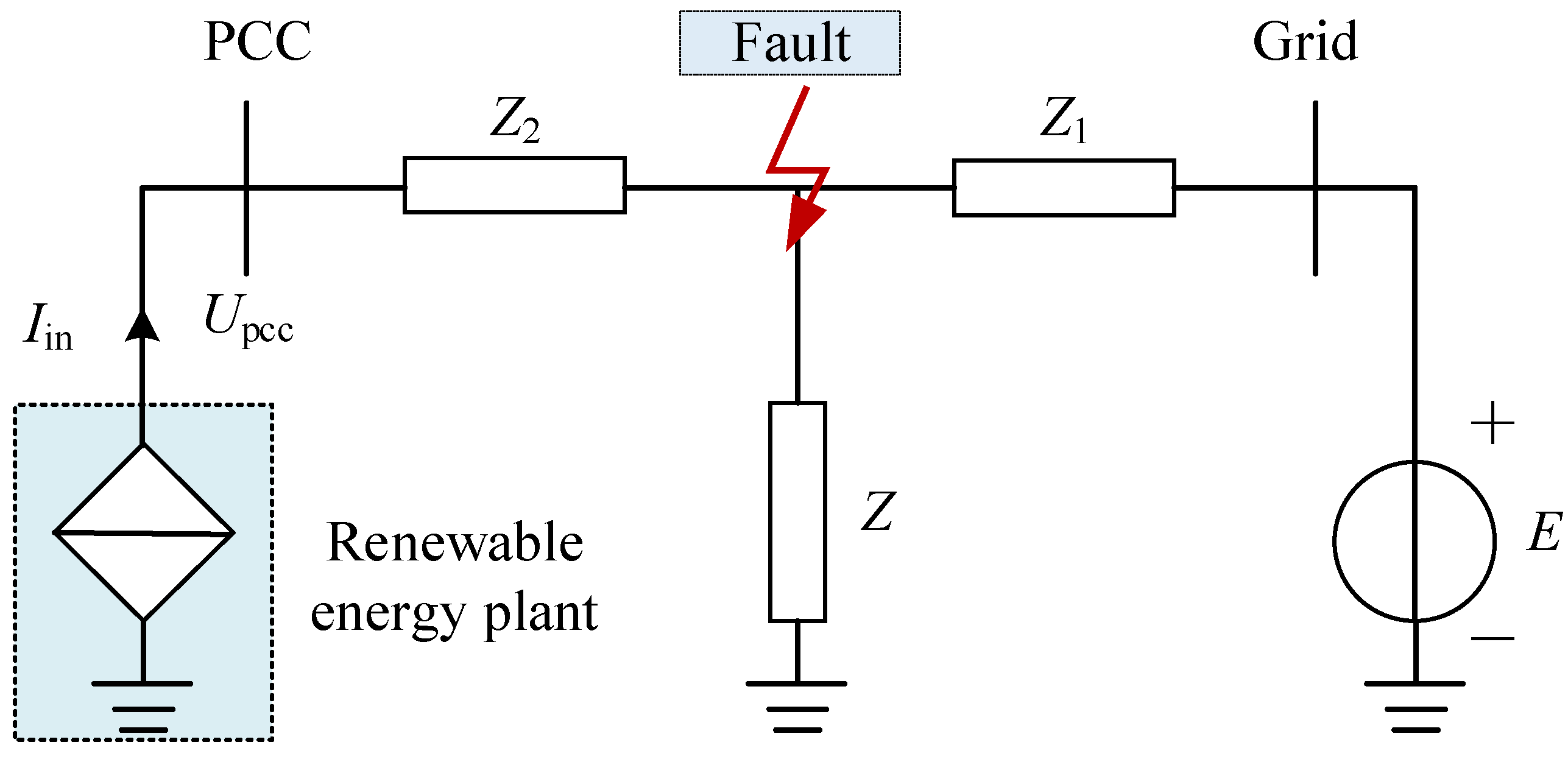
3.1.1. Initial Value Calculation

When a short-circuit fault occurs outside a renewable energy plant, the plant can be considered as a large voltage divider impedance. At this point, the voltage drop at the grid connection point of the renewable energy plant is related to the fault impedance and the system impedance [25,26]. The schematic diagram of an external fault in a renewable energy plant is shown in Figure 3.

In the diagram,

• Z represents the fault impedance;
• Z₁ is the impedance from the fault point to the system;
• Z₂ is the impedance from the renewable energy plant to the fault point;
• E is the voltage amplitude of the infinite bus grid;
• I_in is the current injected by the renewable energy plant into the grid connection point during steady-state fault conditions;
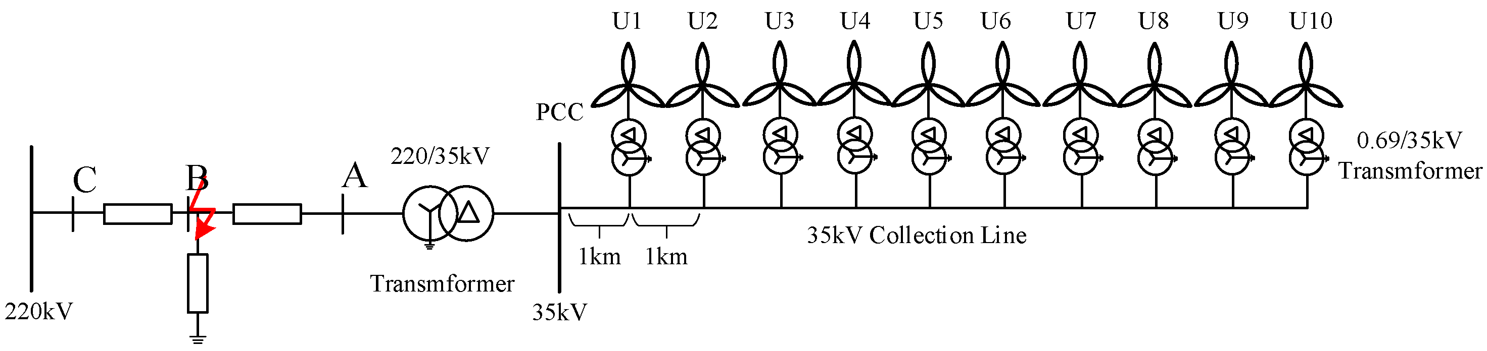
• The red arrow indicates the fault location.

Since the impedance of the transformer is much larger than the line impedance, there is a certain voltage difference between the PCC voltage and the terminal voltage of the N-SMSs inside the plant. However, the voltage difference between different N-SMSs inside the plant is relatively small [24]. Therefore, to quickly assess the status of the renewable energy plant, the voltage U₁ of the N-SMSs closest to the PCC should be calculated. The calculation method is as follows.

To simplify the calculation, the differences between the N-SMSs in the renewable energy plant are neglected, and the plant is treated as a large-capacity N-SMS. During a fault, the reactive power priority control strategy is adopted, and the effect of the active current on the voltage is ignored. According to the Park transformation, the reactive current provided by the renewable energy plant can be calculated based on Equation (9):

$$I_{\mathrm{in}}={\displaystyle \frac{3}{2}}N{I}_{\mathrm{q}}^{*}$$

(11)

where

• N represents the number of N-SMSs in the renewable energy plant.
• I_in is the rated current of the wind farm.

Using the node voltage method, the circuit equation during the fault steady state can be written as

$$(U_1-I_{\mathrm{in}}{Z}_2)({\displaystyle \frac{1}{Z}}+{\displaystyle \frac{1}{Z_1}})={\displaystyle \frac{E}{Z_1}}+I_{\mathrm{in}}$$

(12)

By solving the system of Equations (9), (11) and (12) simultaneously, the voltage U₁ can be obtained as

$$\left\{\begin{array}{cc}{U}_1=U_{\min }+{\displaystyle \frac{3}{2}}N{I}_{\max }{Z}_2& 0.2<U_1\le U_{\mathrm{e}1}\\ U_1={\displaystyle \frac{27K_{1}N{I}_{\mathrm{N}}{Z}_3+20U_{\min }}{30K_{1}N{I}_{\mathrm{N}}{Z}_3+20}}& U_{\mathrm{e}1}<U_1\le 0.9\\ U_{\min }={\displaystyle \frac{Z}{Z+Z_1}}E& \\ Z_3={\displaystyle \frac{Z{Z}_1}{Z_1+Z}}+Z_2& \end{array}\right.$$

(13)

When calculating U₁, it can be initially assumed that it falls within a specific range. The calculation is performed using the formula for that range. If the result contradicts the assumption, the formula for the other range is used. If the result does not contradict, that value is accepted.

Next, it is assumed that the voltages of the remaining N-SMSs also fall within the same range as U₁. Since renewable energy plants often adopt a chain or radial topology [27], the voltage of the other N-SMSs can be calculated using the formula from Equation (13). The calculation steps are illustrated using the chain topology in Figure 4 as an example.

(1)

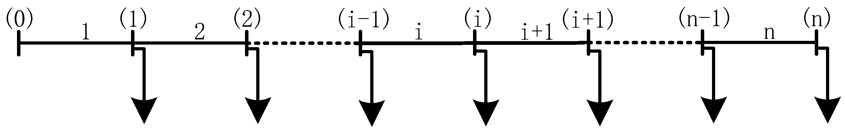
Number the Internal Lines and Nodes of the Renewable Energy Plant.

The first node in the system is the grid connection point (PCC) of the renewable energy plant, numbered as (0). The N-SMS nodes are sequentially numbered from (1) to (n), as shown in Figure 4. The line numbers correspond to the N-SMSs’ number at the line’s terminal. Nodes with numbers smaller than (i) are referred to as upstream nodes of node (i), while those with numbers greater than (i) are called downstream nodes of node (i).

(2)

Calculate the Fault Steady-State Voltage of Each Node.

The calculation method for node (i) is as follows. Following the approach used for single-machine multiplication, given the fault steady-state voltage at node (I − 1), the node (i) and its downstream nodes are equivalently treated as a large N-SMS. Then, using Equation (14), the fault steady-state voltage of node (i) is calculated. By applying this method, the fault steady-state voltages of each N-SMS can be determined sequentially from the PCC voltage.

$$\left\{\begin{array}{cc}{U}_i=U_{i-1}+{\displaystyle \frac{3}{2}}{N}_i{I}_{\max }{Z}_i& 0.2<U_i\le U_{\mathrm{e}1}\\ U_i={\displaystyle \frac{27K_1{N}_i{I}_{\mathrm{N}}{Z}_i+20U_{i-1}}{30K_1{N}_i{I}_{\mathrm{N}}{Z}_i+20}}& U_{\mathrm{e}1}<U_i\le 0.9\end{array}\right.$$

(14)

where

• N_i represents the number of N-SMSs at node (i) and its downstream nodes;
• Z_i is the impedance of the line between node (i) and node (i − 1);
• I_N is the rated current of a single generator;
• U_{i − 1} is the fault steady-state voltage at node (i − 1);
• U_i is the fault steady-state voltage at node (i).

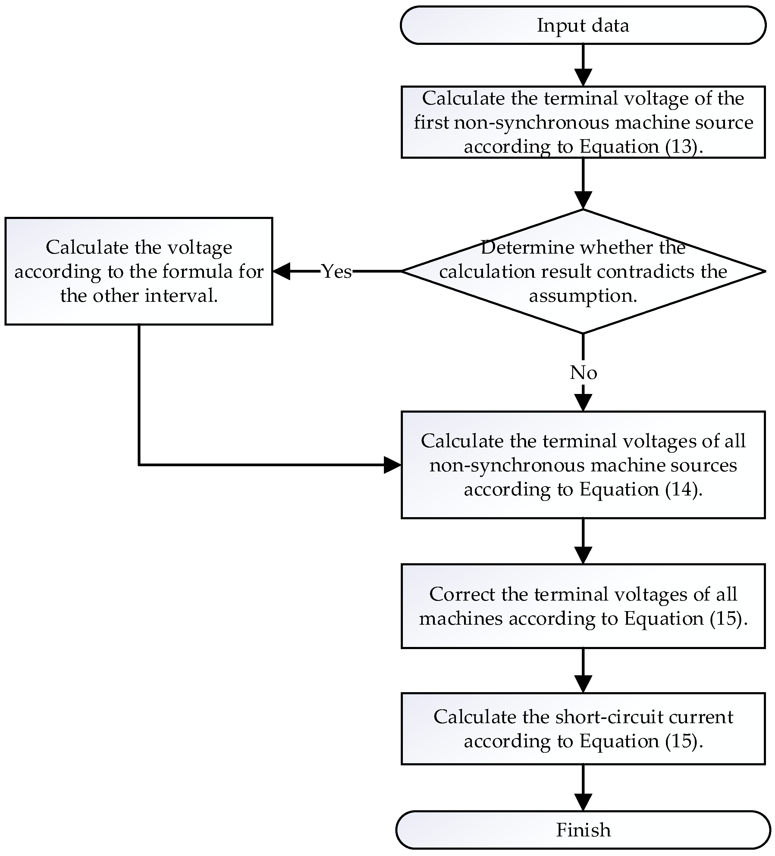
3.1.2. Correction

The initial terminal voltage of the N-SMSs within the renewable energy plant is obtained from Section 3.1.1. However, due to the voltage level of the gathering lines in the plant typically being 35 kV, which does not satisfy the assumption that reactance is much greater than resistance, the voltage calculated without considering the active current is not sufficiently accurate. Nonetheless, it can serve as an initial voltage value for further processing. To avoid iterative calculations, this paper follows a similar approach as before, and, based on the initial voltage, the voltage is corrected. The terminal voltage is calculated using the longitudinal component of the voltage drop, as follows:

$$U_i-U_{i-1}={\displaystyle \frac{P_{i}R+Q_{i}X}{U_{i-1}}}={\displaystyle \frac{3}{2}}({\displaystyle \sum _{j=i}^{\mathrm{N}}{I}_{\mathrm{d},j}^{*}}{R}_i+{\displaystyle \sum _{j=i}^{\mathrm{N}}{I}_{\mathrm{q},j}^{*}}{X}_i)$$

(15)

where

• R_i and X_i represent the resistance and reactance of the line between node (i) and node (i − 1), respectively.
• I_d,j^* and I_d,j^* represent the active and reactive current of the j-th N-SMS, respectively, and can be calculated based on Equation (9).
• i = 0,1,2,…,N, and U₀ = U_min.

Using the voltage magnitude obtained from Equations (9) and (15), the SCCs of all N-SMSs are summed, resulting in the steady-state SCC injected by the renewable energy plant into the grid, given by

$$I={\displaystyle \sum _{i=1}^{\mathrm{N}}{I}_{\mathrm{d},i}^{*}}+j{\displaystyle \sum _{i=1}^{\mathrm{N}}{I}_{\mathrm{q},i}^{*}}$$

(16)

where

• I represents the SCC injected by the renewable energy plant into the grid.

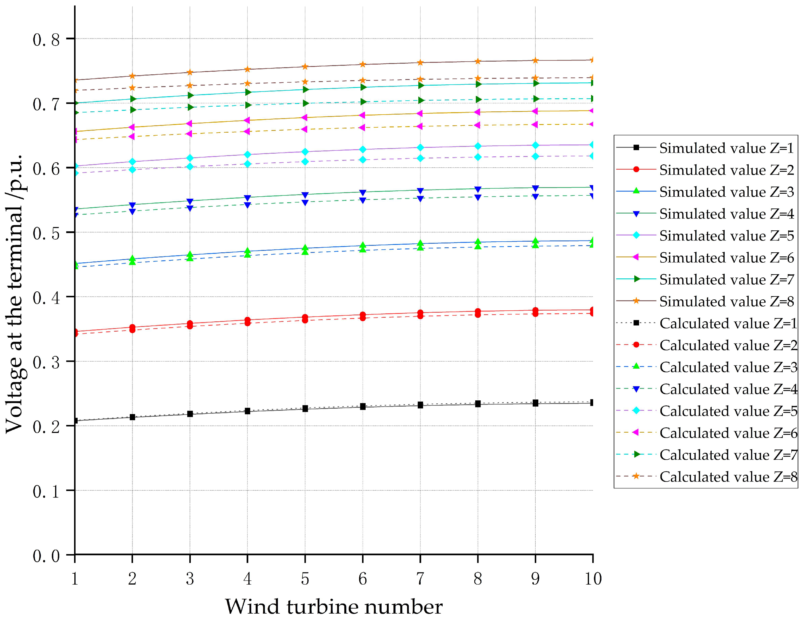
Based on the above, the SCC calculation process for the new energy power plant is shown in the Figure 5.

4. Results

To validate the feasibility of the method proposed in this paper, a detailed model of the renewable energy plant, as shown in Figure 6, was constructed in PSCAD/EMTDC in conjunction with practical engineering considerations. The plant primarily consists of wind turbines, a back-to-back converter, a box transformer, and a main transformer. The wind turbines are connected to the box transformer (0.69 kV/35 kV) via the back-to-back converter and then aggregated through the collection lines to the 35 kV bus. From there, the power is transmitted to the 220 kV system via the main transformer (35 kV/220 kV) for grid connection. The red arrow in Figure 6 is the fault position.

Due to the similarity of the collection lines, the case study includes a permanent-magnet direct-drive wind farm with the following specifications: 1 (number of collection lines) × 10 (number of turbines per collection line) × 2 MW (rated capacity of each generator). The turbine spacing is set to 1 km, and the basic wind speed is set to 10 m/s. The main parameters of the wind farm are shown in

Table 1. Main component parameters of permanent-magnet wind field.

Type	Parameter	Value
35 kV line	Impedance	0.13 + 0.23 jΩ/km
Box-type transformer	Transformation ratio	0.69/35 kV
	Capacity	2.24 MW
	Impedance	6.39%
Main transformer	Transformation ratio	35/220 kV
	Capacity	100 MW
	Impedance	13.54%

. The grid-connected inverter adopts the control strategy presented in Section 1. The control strategy in steady-state is shown in Figure 1, while the LVRT strategy during faults is described in Section 2.2. The wind turbine component models the simple mechanical physics of a wind turbine, considering blade configuration (two or three blades), tip speed ratio, coefficient of power, and blade sweep area and radius. Shaft dynamics are not considered in this model, and it may be used together with the wind governor model. Its main parameters are shown in

Table 2. Main parameters of wind turbine.

Parameter	Value
Generator-rated MVA	2.2419/MVA
Machine-rated angular speed	314.15927/rad/s
Rotor radius	41.2/m
Rotor area	5333/m2
Air density	1.229/kg/m3
Gearbox efficiency	1.0/pu

.

At t =1 s, a three-phase short-circuit fault is applied, with the fault point located at the red arrow in Figure 6. The fault lasts for 0.5 s. The equivalent impedances of line segments AB and BC are (0.4860 + 1.3820 j) Ω and (1.9440 + 5.5280 j) Ω, respectively. Different fault impedances are set, and the steady-state fault voltage at the terminals of each wind turbine is calculated using the methods proposed in Section 3. The results are compared with the simulation outcomes, as shown in Figure 7 and

Table 3. Maximum voltage error of wind.

Short-Circuit Impedance/Ω	Maximum Wind Turbine Voltage Relative Error/%
1	0.99
2	−1.48
3	−1.59
4	−2.25
5	−2.73
6	−3.05
7	−3.35
8	−3.55

. The steady-state SCC injected into the fault point by the wind farm is provided in

Table 4. The short-circuit current of the wind farm.

Short-Circuit Impedance/Ω	Simulation Value/kA	Single-Machine Multiplication Calculation Value/kA	Single-Machine Multiplication Relative Error/%	Iterative Method Calculation Value/kA	Iterative Method Relative Error/%	Proposed Method Calculation Value/kA	Proposed Method Relative Error/%
1	0.0635	0.0616	−3.02	0.0624	−1.76	0.0616	−3.02
2	0.0627	0.0616	−1.80	0.0621	−1.01	0.0612	−2.44
3	0.0617	0.0616	−0.14	0.0611	−0.95	0.0609	−1.27
4	0.0545	0.0574	5.32	0.0547	0.37	0.0545	0.00
5	0.0495	0.0519	4.92	0.0495	0.07	0.0496	0.27
6	0.0459	0.0479	4.39	0.046	0.25	0.0461	0.47
7	0.0429	0.045	4.83	0.0433	0.87	0.0436	1.57
8	0.0412	0.0429	4.13	0.0415	0.73	0.0418	1.46

.

The method for calculating the errors in Table 2, Table 3 and Table 4 is as follows:

$$relative error={\displaystyle \frac{calculated value-simulated value}{simulated value}}\times 100\%$$

(17)

The relative error represents the difference between the calculated value and the simulated value. A smaller relative error indicates a higher accuracy of the method.

It can be observed that under different short-circuit impedances, the steady-state fault voltage at the terminals of the wind turbines calculated using the proposed method shows that the maximum voltage error did not exceed 3.02%, which was relatively small. This indicates that the method proposed in this paper has good accuracy. The main source of error arose from the calculation of the initial terminal voltage, where the impact of the active current on the voltage was neglected. Additionally, the single-machine multiplication method was used. Although voltage correction was subsequently applied, some error remained. The relative error in voltage was larger when the voltage drop was smaller because, in cases of smaller voltage drops, the proportion of the active current was higher. Therefore, neglecting the impact of the active current on the calculation of the initial terminal voltage naturally led to larger errors.

In addition, the forward–backward substitution method from reference [26] was also applied to calculate the SCC of the wind farm. This method has a smaller relative error compared with the proposed method in this paper, but it requires iterative computation, and its time complexity is several times higher than that of the proposed method in this paper.

Currently, the main method for calculating the short-circuit current of renewable energy stations is still the single-machine multiplication method. In all, the accuracy of the SCC calculated using the proposed method showed a significant improvement over the single-machine multiplication method, with errors within an acceptable range, thus verifying the feasibility of the method proposed in this paper.

5. Conclusions

This paper proposes a practical method for calculating the SCC in renewable energy plants. This method does not require iterative calculations, offers high accuracy, and demonstrates strong engineering applicability. The maximum error does not exceed 3.02%, slightly higher than the iterative method. However, the method has much lower time and space complexities. It strikes a good balance between accuracy and resource efficiency. Although the method was validated using a wind farm as an example, it is equally applicable to photovoltaic power plants and energy storage plants with similar control strategies.

However, there are some limitations to this approach. First, the method only considers the SCC in the steady state after the fault, which is the current practice in engineering. Second, it only accounts for the SCC under positive-sequence symmetrical faults, without considering asymmetrical faults. In fact, single-phase short-circuit faults are the most common type of fault in power systems. The method proposed in this paper only considers the SCC under symmetric fault conditions. To extend this method to asymmetric faults, sequence network analysis would need to be incorporated, allowing for the consideration of both negative-sequence and zero-sequence SCCs. This aspect will be explored in future research. Lastly, this method is only applicable to chain or radial topologies and may not be suitable for ring-type collection topologies.

References

1. Li, M. Characteristic Analysis and Operational Control of Large-Scale Hybrid UHV AC/DC Power Grids. Power Syst. Technol. 2016, 40, 985–991. [Google Scholar] [CrossRef]
2. Yang, P.; Liu, F.; Jiang, K.; Mao, H. Large-disturbance stability of power systems with high penetration of renewables and inverters: Phenomena, challenges, and perspectives. J. Tsinghua Univ. (Sci. Technol.) 2021, 61, 403–414. [Google Scholar] [CrossRef]
3. Xie, X.; He, J.; Mao, H.; Li, H. New Issues and Classification of Power System Stability with High Shares of Renewables and Power Electronics. Proc. CSEE 2021, 41, 461–475. [Google Scholar] [CrossRef]
4. Wei, C. Key Technology Research and Application of Modern Power System Short-Circuit Current Practical Calculation. Dissertation Thesis, Shanghai University, Shanghai, China, 2018. [Google Scholar] [CrossRef]
5. Li, T. Calculation of Short Circuit Fault Current in Power System with a Large Number of Inverter-Interfaced Sources. Dissertation Thesis, North China Electric Power University, Beijing, China, 2024. [Google Scholar] [CrossRef]
6. Kong, X.; Yuan, Y.; Huang, H.; Zhu, W.; Li, P.; Wang, Y. Fault Current Transient Features and Its Related Impact Factors of PV Generator. Power Syst. Technol. 2015, 39, 2444–2449. [Google Scholar] [CrossRef]
7. Xu, K.; Zhang, Z.; Liu, H.; Liu, W.; Ao, J. Study on Fault Characteristics and Its Related Impact Factors of Photovoltaic Generator. Trans. China Electrotech. Soc. 2020, 35, 359–371. [Google Scholar] [CrossRef]
8. Fan, X.; An, D.; Sun, S.; Sun, D.; Wang, Y. Three-Phase Short Circuit Current Characteristic Analysis of Doubly Fed Induction Generator Considering Crowbar Protection Action Time. Trans. China Electrotech. Soc. 2019, 34, 3444–3452. [Google Scholar] [CrossRef]
9. Linghu, T.; Han, M.; Huo, Q.; Tang, X. Equivalent Modeling of Doubly-Fed Wind Farms Short-Circuit Current Calculation Considering Different Fault Ride-Through Modes. South. Power Syst. Technol. 2022, 16, 28–37. [Google Scholar] [CrossRef]
10. Yin, J.; Bi, T.; Xue, A.; Yang, Q. Study on Short-circuit Current and Fault Analysis Method of Hybrid Wind Farm with Low Voltage Ride-through Control Strategy. Trans. China Electrotech. Soc. 2015, 30, 99–110. [Google Scholar] [CrossRef]
11. Song, J.; Cheah-Mane, M.; Prieto-Araujo, E.; Gomis-Bellmunt, O. Short-Circuit Analysis of AC Distribution Systems Dominated by Voltage Source Converters Considering Converter Limitations. IEEE Trans. Smart Grid 2022, 13, 3867–3878. [Google Scholar] [CrossRef]
12. Jia, K.; Hou, L.; Bi, T.; Li, Y.; Qin, H.; Ding, X. Practical Engineering Calculation of Short-circuit Current for Renewable Energy Based on Local Iteration of Fault Area. Autom. Electr. Power Syst. 2021, 45, 151–158. [Google Scholar] [CrossRef]
13. Hong, S.; Fan, C.; Chen, S. Research on Fault Equivalence Method for Multiple Inverter-Interfaced Distributed Generation Based on PQ Control Strategy. Power Syst. Technol. 2018, 42, 1101–1109. [Google Scholar]
14. Jin, Y.; Wu, D.; Ju, P.; Rehtanz, C.; Wu, F.; Pan, X. Modeling of Wind Speeds Inside a Wind Farm with Application to Wind Farm Aggregate Modeling Considering LVRT Characteristic. IEEE Trans. Energy Convers. 2020, 35, 508–519. [Google Scholar] [CrossRef]
15. Wu, Z.; Cao, M.; Li, Y. An Equivalent Modeling Method of DFIG-based Wind Farm Considering Improved Identification of Crowbar Status. Proc. CSEE 2022, 42, 603–614. [Google Scholar] [CrossRef]
16. Mi, Z.; Su, X.; Yang, Q.; Wang, Y. Multi-Machine Representation Method for Dynamic Equivalent Model of Wind Farms. Trans. China Electrotech. Soc. 2010, 25, 162–169. [Google Scholar] [CrossRef]
17. Xu, Y.; Liu, D. Equivalence of wind farms with DFIG based on two-step clustering method. Power Syst. Prot. Control 2017, 45, 108–114. [Google Scholar] [CrossRef]
18. Ye, L.; Shi, Y.; Wang, W.; Peng, Y.; Pei, M. Multi-step Grouping and Equivalent Modeling of Distributed Photovoltaic Clusters for Transient Analysis. Autom. Electr. Power Syst. 2023, 47, 72–81. [Google Scholar] [CrossRef]
19. Zhou, Y.; Zhao, L.; Hsieh, T.Y.; Lee, W.J. A Multistage Dynamic Equivalent Modeling of a Wind Farm for the Smart Grid Development. IEEE Trans. Ind. Appl. 2019, 55, 4451–4461. [Google Scholar] [CrossRef]
20. Qi, J.; Li, W.; Cao, P.; Li, Z. Practical equivalent method for direct-driven wind farm. Electr. Power Autom. Equip. 2022, 42, 50–57. [Google Scholar] [CrossRef]
21. Han, W.; Liu, S.; Xiao, C.; Liu, Y.; Song, C.; Wang, Z. Steady short-circuit calculation model for a photovoltaic station considering different generation units’ fault characteristics. Power Syst. Prot. Control 2021, 49, 129–135. [Google Scholar] [CrossRef]
22. Li, P.; Huang, Y.; Wang, G.; Li, J.; Lu, J. A Short-Circuit Current Calculation Model for Renewable Power Plants Considering Internal Topology. Appl. Sci. 2024, 14, 10745. [Google Scholar] [CrossRef]
23. GB/T 19963.1-2021; Technical Specification for Connecting Wind Farm to Power System; Part 1: On Shore Wind Power. Publisher Standards Press of China: Beijing, China, 2021.
24. Tang, Y.; Song, G.; Hao, Z.; Jiang, J.; Chang, N.; Lang, X. Practical Calculation Method for Fault Steady-state Current in Inverter-interfaced Generator Stations. Autom. Electr. Power Syst. 2024, 48, 182–191. [Google Scholar]
25. Sun, H.; Li, J.; Li, W.; Guo, J.; An, N.; Zhang, Y. Research on Model Structures and Modeling Methods of Renewable Energy Station for Large-scale Power System Simulation (II): Electromechanical Transient Model. Proc. CSEE 2023, 43, 2190–2202. [Google Scholar] [CrossRef]
26. Li, D.; Shen, C.; Wu, L.; Chen, X.; Yang, Y. Study on Fault Response Characteristics Classification and Discriminant Method of PMSG Considering Initial Wind Speed and Drop Degree of Terminal Fault Steady-state Voltage. Proc. CSEE 2024, 44, 1247–1260. [Google Scholar] [CrossRef]
27. Yang, Y. Study on Topology Structure of Large Wind Power Base. Dissertation Thesis, North China Electric Power University, Beijing, China, 2017. [Google Scholar] [CrossRef]
Figure 1. Diagram of grid-following N-SMS and its control system.
Electricity 06 00007 g001
Figure 2. SCC amplitude curve.
Electricity 06 00007 g002
Figure 3. External fault of renewable energy plant.
Electricity 06 00007 g003
Figure 4. Renewable energy plant internal loop.
Electricity 06 00007 g004
Figure 5. SCC calculation flowchart for renewable energy plants.
Electricity 06 00007 g005
Figure 6. Sketch diagram of the detailed wind farm model.
Electricity 06 00007 g006
Figure 7. Fault steady-state voltage of each wind turbine.
Electricity 06 00007 g007