Abstract
This paper presents a detailed fifth-order mathematical model of a three-phase induction motor, used in the WECC (Western Electricity Coordinating Council) composite load model. The main objective is to analyze the dynamic behavior of three-phase induction motors during fault-induced delayed voltage recovery (FIDVR) events, a critical phenomenon in power system voltage stability. The model is implemented in MATLAB/Simulink and validated by comparing its results with previous studies, demonstrating its ability to capture transient and subtransient responses under voltage disturbances. Different types of motors (A, B, and C) are analyzed, and variations in load and voltage disturbance magnitudes are studied. The results show that the model is accurate and robust, making it useful for voltage stability studies in systems with high induction motor penetration. However, the model has limitations, such as the lack of consideration for frequency drives and protection systems, suggesting areas for future research.
1. Introduction
The stalling of three-phase induction motors during a system fault and the resulting low voltages on the grid contribute significantly to the problem of fault-induced voltage-delayed recovery (FIDVR) [1,2,3]. During the time that the motors are exposed to these low voltages, they typically slow down and begin to consume increasing amounts of reactive power. This creates additional voltage drops, which prevent full and rapid recovery to normal voltage levels [4].
The accurate prediction of the dynamic behavior of three-phase induction motors during FIDVR events poses significant challenges that conventional static and dynamic models are unable to adequately address [5]. As three-phase induction motors account for 70% of electricity consumption [6,7,8], the development of an accurate load model is imperative for comprehending the dynamic behavior of motor loads in power systems and for conducting preemptive analyses of voltage stability in the grid [9,10].
A comprehensive compendium of models has been developed, offering a comprehensive overview of the state of the art in modeling three-phase induction motors as system load [11]. This compendium encompasses a wide range of models, including static models, which, according to Smart [11], are employed in scenarios where the transient response is deemed non-pertinent for the analyses conducted. Additionally, dynamic models are utilized in instances where it is imperative to consider studies related to transient phenomena and system stability over brief periods.
On 10 August 1996, the power system of the United States (U.S.) experienced a significant blackout event that resulted in the division of the system into four distinct islands. This incident led to the loss of 30.390 MW and the disruption of electricity services for 7.49 million customers across western North America [11,12,13]. This event catalyzed the development of the classical ZIP + IM composite load model, a methodology employed to assess load conditions by analysing the dynamic effects of high peak summer voltage conditions [11,14,15,16,17].
The equivalent of this model is composed of the ZIP model, which associates a constant impedance (Z), constant current (I), and constant power (P) component, in addition to the third-order dynamic model of the induction motor [3,11]. Research findings indicate that this model successfully captures the dynamics of the primary system loads. However, its efficacy in capturing delayed voltage recovery events (FIDVR) is limited [18].
As electrical systems undergo continuous evolution, the proportion of built-in induction motor loads experiences a corresponding increase, integrating novel automation technologies and exerting a significant impact on energy demand [3]. The increasing trend in demand necessitates models capable of accurately and completely representing the dynamic behavior of power demand in the face of grid failures.
Presently, the most recent WECC (Western Electricity Coordinating Council) composite load model [1,17,19] is the most popular and accurate composite load model [7]. This is due to the fact that it includes a wide variety of three-phase motors, single-phase motors, and electronic components. This gives it the flexibility to capture specific characteristics with different loads [5,14,19].
The WECC model is available in computational tools for the development of electromechanical transient studies, such as GE PSLF, Power World Simulator, and PSSE [5,14,19,20,21]. However, the technical methods and mathematical representations for developing the model of these loads are not publicly available in simulation programs [19]. Consequently, the development of induction motor models is limited in its ability to anticipate critical events, optimize resource utilization, and reduce losses in a specific power grid [9].
As stated in [22], the WECC composite load model has developed a block diagram derived from the fifth-order three-phase motor model for the transient and subtransient analysis of induction motors. This diagram considers the stator and rotor circuit transients, along with the rotor speed transient [8].
The fifth-order model is the most commonly used model for three-phase induction motors. This is due to its ability to model large motors and take into account the load response [11]. The model comprises five differential equations that delineate the behavior of the stator, rotor, and rotor speed within the direct-axis and quadrature-axis () systems [23]. A distinguishing feature of this approach is its ability to effectively capture the dynamic state of the stator, a capability that the third-order model lacks [8].
A number of studies have approached the fifth-order induction motor model. Of particular note is the work of [18], who, in addition to representing the components of each of the WECC loads, used the fifth-order model to analyze the behavior of the three types of three-phase induction motors against a voltage perturbation. Additionally, [4] has made a noteworthy comparison between the fifth-order model in the time domain and the steady-state Quasi-AC model. This comparison was made to analyze the efficiency of the representation in the presence of a voltage disturbance when the connected load changes.
These scientific efforts have contributed to the knowledge of the three-phase induction motor model. However, the nonlinear nature of the structure, as defined by the five-state method, introduces challenges in the direct application of analytical approaches for the calculation of partial derivatives [20]. This paper presents a detailed mathematical procedure to implement the fifth-order three-phase induction motor model used by WECC and calculate its transient and subtransient responses by analyzing the impact of the voltage drop disturbance to the FIDVR phenomenon.
The mathematical model was implemented in Simulink MATLAB (version 2024b) to analyze the dynamic responses of a three-phase induction motor. The objective was not only to facilitate the analysis of the community’s fifth-order model of the induction motor against voltage disturbances, but also to provide a detailed mathematical representation of the model. The present paper proposes a detailed mathematical model of the three-phase induction motor of fifth order in the direct and quadrature () axis. The implementation of the block diagram of the three-phase induction motor model adopted by WECC in Simulink is also presented. The model’s implementation is validated by analyzing the behavior of the induction motor in response to variations in motor type, load type, and voltage disturbance magnitude
The contributions will be presented in the body of this manuscript as follows: The initial section of the paper presents the methodology for the implementation of the mathematical modeling of the three-phase induction motor as a WECC load, and for the validation of the model against different variations. The subsequent section presents the results of the simulations of the implemented model, demonstrating the dynamics at start-up and in the presence of delayed voltage recovery disturbances. Finally, the fourth section presents the conclusions of the implementation and simulation results, addressing the validation of the proposed model and its limitations.
2. Materials and Methods
2.1. Composite Load Model WECC
The WECC model (see Figure 1) incorporates an electrical representation of a distribution system, comprising a substation transformer and a feeder equivalent. With respect to the distribution system, the model includes a static load model, a power electronics model, three three-phase motor models, a single-phase A/C motor, and a DER.
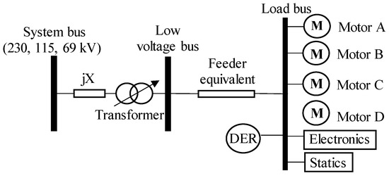
Figure 1.
WECC composite load model structure.
As illustrated in Figure 1, distributed energy resources (DERs) are defined as distributed generation loads, including solar photovoltaic panels, small wind generation systems, and small hydroelectric power plants. Static loads, on the other hand, are defined as resistive distribution loads and are represented by the ZIP model. The electronics loads, which are the power electronics loads with the greatest impact on the system [11], are of interest. The motor loads are represented by three three-phase induction motors and one single-phase induction motor, which possess the following characteristics [18,24]:
- Motor A: Single-cage induction motor, represents motors with low inertia driving constant torque loads.
- Motor B: Deep squirrel-cage induction motor, represents motors with high inertia driving variable torque loads
- Motor C: Double squirrel-cage induction motor, represents motors with low inertia driving variable torque loads.
- Motor D: Single-phase motor, represents heating, ventilation, and air conditioning systems.
2.2. Mathematical Model of the Three-Phase Induction Motor
A fifth-order system has been utilized in previous studies [5,18,19,22] for the analysis of electromechanical transients in three-phase induction motors within the Western Electricity Coordinating Council (WECC) composite load model [8]. The mathematical model is frequently employed for the representation of a motor C [19]. However, it is also applicable to other types of three-phase induction motors, including Motor A and Motor B [18].
As shown in Figure 2, the block diagram presents a comprehensive representation of the electromechanical parameters of the induction motor. This motor is represented by five state variables [19,22]. These variables include the transient and subtransient voltages in the direct and quadrature axes (, , and ), as well as the rotor slip (). The model accurately describes the dynamic behavior of the motor by integrating these state variables into a system of differential equations that describe the interactions between the electrical and mechanical components.
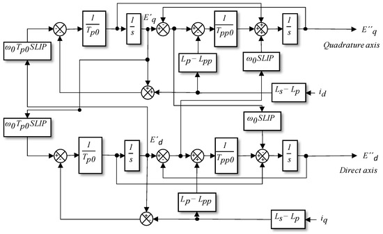
Figure 2.
Block diagram for the fifth-order model of the induction motor.
The input parameters necessary to simulate the induction motor model presented in Figure 2 are enumerated in Table 1, as outlined in [1]. This subsection presents a systematic approach to determine these parameters, which are essential to accurately represent the dynamic behavior of three-phase induction motors within the fifth-order mathematical framework adopted by WECC.

Table 1.
Parameters proposed by WECC for the induction motor model.
The electrical representation of the model is described by four state variables on the direct and quadrature axes (), as detailed in [18] and expressed in Equations (1)–(4). These variables are the transient and subtransient voltages of the direct and quadrature axes (, , and ), which are essential for modeling phenomena such as motor starting, short circuits, and frequency variations [19].
In this context, the symbol represents the synchronous speed in radians per second. , , and denote the synchronous, transient, and subtransient inductances per unit, respectively. The rotor transient and subtransient time constants, and , respectively, are defined as the time response of the rotor flux linkages to changes in stator voltage [1]. These parameters are extracted from the unit equivalent circuit of the induction motor, as illustrated in Figure 3 [6,18,23,25].
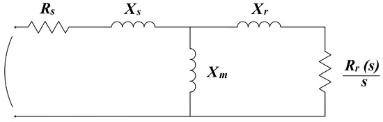
Figure 3.
Equivalent circuit diagram of a motor with single cage rotor or deep bar rotor.
In the equivalent circuit of an induction motor (see Figure 3), the parameters , , , , , and s represent the stator resistance, stator-referenced rotor resistance, stator leakage reactance, stator-referenced rotor leakage reactance, magnetizing reactance, and slip, respectively [8].
In order to facilitate a comparison and analysis of induction motors of different power ratings, it is common to express these parameters in per-unit values. As previously mentioned in [2,6,8,26], the per-unit system provides a normalized representation of the machine. This allows for the development of generalized models and facilitates the analysis of power systems. The conversion of an ohms parameter to per unit is achieved by dividing it by the corresponding base impedance, as outlined in Equation (5). This approach aligns with the established convention stipulating that the base impedance is itself the base impedance. This is consistent with the established convention [6]. The base impedance is typically calculated from the nominal voltage and apparent power of the machine.
Z represents the impedance in ohms. The base voltage and base power ( and ) are derived from the motor nameplate data. The equivalent circuit in per unit is then employed to define the parameters outlined in Equations (6)–(8). For type A and B motors, it has been demonstrated that the parameters ( = 0) and ( = 0) hold true, as illustrated in [22].
In the case of the double cage design, which implies the presence of two resistors (, ) and two reactances (, ) connected in parallel, the values of and are determined from Equations (9) and (10) [2].
As can be seen in Figure 2, the model inputs are the direct and quadrature axis currents (, ), which are derived from Equations (11) and (12) [18,19,27].
The direct and quadrature axis voltages (, ) represent the components of the input voltage on the axes of the model. The magnitude of the voltage, denoted by |V|, is calculated as the square root of the sum of the squares of the direct and quadrature axis voltages, and , respectively [28]. It is therefore proposed to set equal to zero and leave equal to the unit value of the voltage magnitude; that is, ( = 1) for nominal voltage operation [29].
The fifth state variable is the rotor slip (), defined in Equation (13). This variable is critical for modeling the dynamic behavior of induction motors, as it is directly related to the torque speed characteristics [11,18,23]. The inertia constant, denoted by H, signifies the motor’s capacity to accumulate kinetic energy and is measured in seconds [30,31].
The load torque (), as delineated in Equation (14), is expressed as a function of the mechanical speed, () (expressed as a fraction of the synchronous speed, 1-slip, according to [18]. The coefficientsA, B, C, and D are assigned specific values and are intended to represent distinct components of the load. These components are defined as follows: () represents a quadratic component of the velocity, () represents a linear component, (C) represents a constant component, and (D) represents a component related to mechanical losses [5,6,18]. The term is a coefficient that associates mechanical damping, considering friction, and winding losses.
The initial mechanical torque (), as specified by Equation (15), signifies the initial mechanical load of the motor and is derived through the utilization of the initial subtransient voltages and currents in the direct and quadrature axes [5,18,19].
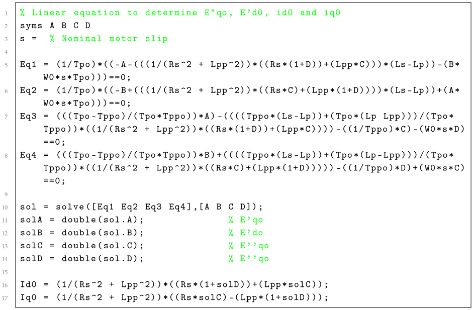
The initial conditions (, , and ), are determined from the initial state (, ) of the system. These initial conditions are obtained by numerically solving the motor equations (Equations (1)–(4)) using the method described in Appendix A [19,27].
As specified in Equation (16), the electric torque () denotes the electromagnetic torque generated by the motor.
The active power (P), which represents the real power supplied to the load, and the reactive power (Q), associated with the energy stored in the magnetic field [24], are calculated by Equations (17) and (18), which express P and Q in terms of the direct and quadrature axis components of the voltage and current (, , , )
2.3. Simulink Model Implementation
A block diagram representing a three-phase induction motor as a load for the WECC model was implemented in MATLAB/Simulink (see Figure 2) [8,11,18,19,32,33]. The direct and shaft quadrature currents (, ) were calculated based on the motor equivalent circuit parameters, as illustrated in the block diagram in Figure 4. The stator re-ignition current () and stator re-ignition current () were calculated based on the motor equivalent circuit parameters. The stator resistance () and rotor leakage inductance () were obtained from the nameplate or data sheet of the motor and are tabulated in Table 1. To simulate various operating conditions, direct and quadrature shaft voltages (Vd, Vq) were applied to the motor model as inputs.
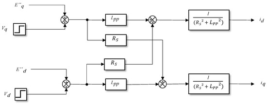
Figure 4.
Block diagram for determination of Id and Iq.
The efficiency of the induction motor is influenced by the rotor slip (). The calculation of the rotor slip is based on the block diagram illustrated in Figure 5, determined by Equation (13).
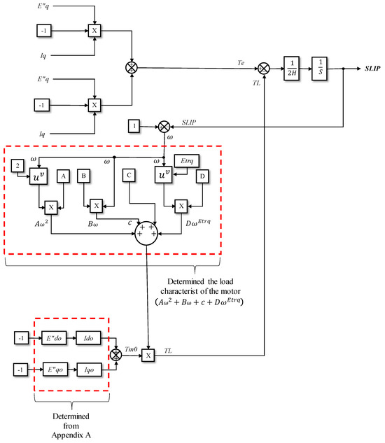
Figure 5.
Block diagram for SLIP determination (Appendix A).
Once the Simulink model has been implemented, a simulation is performed to examine the motor starting process. To represent the components (, ), two step input blocks are incorporated. The component is maintained at a constant value of zero, while the component is initialized to zero and subsequently undergoes a unit step change at the one-second mark.
2.4. Validation of the Implemented Model
2.4.1. Parameter Variation
A validation process is implemented to evaluate the accuracy of the three-phase induction motor model using the parameters of the type A, B, and C motors. The parameters used for each type of three-phase motor are taken from [18] and presented in Table 2. A simulated delayed voltage recovery disturbance is then subjected to the inputs (, ). Subsequently, the resulting active and reactive power outputs are compared with the corresponding values shown in [18].
Table 2.
Type A, B, and C motor parameters.
The voltage perturbation, which is outlined in [18], is expressed through the following mathematical Equation (19). In this equation, the parameters a, b, c, and d correspond to the amplitude of the voltage drop, the duration of the drop, the ramp recovery time, and the initial ramp recovery level, respectively.
2.4.2. Motor Load Variation
A comparative study was carried out with the results reported in [4]. The study involved varying the load applied to a 2-pole, 460 V, 50 HP, 60 Hz squirrel cage induction motor (Motor A). The static parameters of this motor are presented in Table 3.
Table 3.
Electrical parameters of Motor A.
Two simulation scenarios were performed using motor A as a case study. The first scenario was under no-load conditions, . The second scenario was under a constant load, , . In both cases, once the motor reached its rated speed, a disturbance consisting of a 75% decrease in terminal voltage at 5 s was introduced. After this disturbance, the voltage recovered to its rated level at 5.2 s. Thereafter, the system was permitted to revert to its steady-state conditions. The model implemented will consider the constants D and , defined in Equation (14). Given the designation of the motor as type A, the values and were set.
2.4.3. Variation in Voltage Disturbance Magnitude
In order to validate the response of the induction motor model during voltage disturbances, a simulation of voltage drops of 85%, 65%, and 45% with respect to the nominal voltage of motor B in Table 2 was carried out.
Perturbations are applied to motor when they are in a stable state. An undervoltage is applied in one second during the simulation, and this is recovered in one millisecond. The behavior of the active and reactive power, as well as the speed of the motor, will be analyzed.
3. Results and Discussion
3.1. Simulation of Motor Start-Up
In order to assess the performance of the model, the parameters of Motor B in Table 2 are utilized. A step input of 1.0 p.u. is applied to the direct shaft voltage () one second after the initiation of the simulation. This enables the analysis of the transient response of the electrical and mechanical torques, as well as the rotor speed, during motor start-up.
As previously outlined in [4,23,24,32], the initial phase of the electrical torque’s operation exceeds the mechanical torque, which enables the motor to accelerate against its inertia and load torque. As can be seen in Figure 6, the maximum electrical torque of 2.48 p.u. is achieved after 1.58 s. Subsequently, the mechanical torque gradually increases to match the electrical torque at 2.2 s into the simulation.
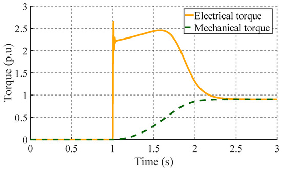
Figure 6.
Electrical torque and mechanical torque of the motor during start-up.
As presented in Figure 7, the speed response of the motor displays a conventional characteristic of induction motors, reaching its rated speed at non-zero slip. The simulated acceleration time of 2.2 s during motor startup is consistent with that expected based on motor parameters and applied load. The influence of the model on the motor’s dynamic response is evident in the smooth acceleration profile and steady-state speed.
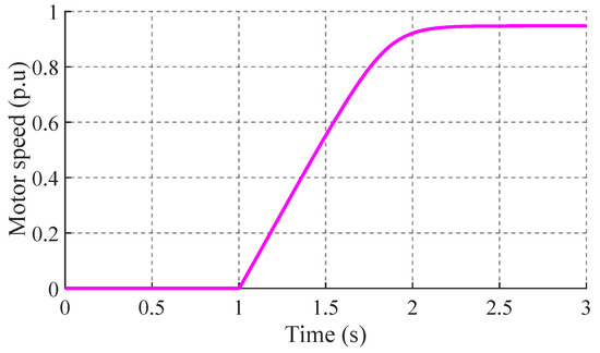
Figure 7.
Speed of the motor during start-up.
The analysis of Figure 6 and Figure 7 reveals a response consistent with the established dynamic characteristics of the three-phase induction motors. The simulated results exhibit numerical stability and closely align with the predicted behavior of induction motors under load conditions, thus supporting the robustness of the proposed model.
3.2. Validation of the Implemented Model
3.2.1. Parameter Variation
In order to validate the model, a delayed voltage recovery perturbation, defined in Equation (19) and illustrated in Figure 8, was applied to the implemented motor model. The simulated responses of the direct and quadrature axis voltages (, ) were then compared with the results presented in [18] for type A, B, and C motors. The model validation results are suitable for voltage stability studies, especially in systems with significant induction motor loads.
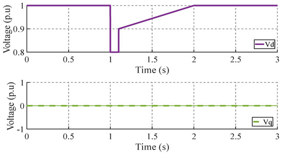
Figure 8.
Direct and quadrature axis voltage ( and ).
Validation of Motor A
As illustrated in Figure 9, the active power response of motor A simulated using the proposed model is compared with the results reported by Zixiao Ma in [18]. Although both models show a comparable response to the voltage disturbance, disparities arise in the magnitude of the power peaks; the Zixiao Ma model reaches a peak recovery no greater than (1.2 p.u.), while in the implemented model it reaches a peak greater than (1.5 p.u.). These discrepancies could be attributed to the characteristics of the load connected to the motor. In the case that the models consider simplified or nonlinear loads, this could lead to variations in the dynamic response of the system. For example, a load with a high harmonic content could influence the motor response in each model in a different way.
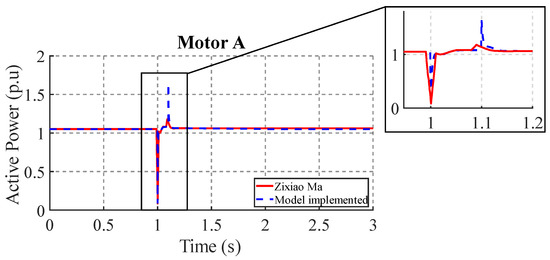
Figure 9.
Active power response in motor A.
As observed in Figure 10, the reactive power response of motor A to the voltage disturbance is analogous in both models. It is evident that both models, the proposed one and Zixiao Ma model, exhibit numerically alike behavior with respect to their response. However, discrepancies emerge in the magnitude of the maximum reactive power peak and the time its occurrence is manifested. Specifically, the Zixiao Ma model exhibits an impulse of 0.8 p.u., temporally displaced by 0.1 ms, while the implemented model displays an impulse of 1.1 p.u.
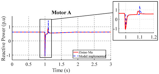
Figure 10.
Reactive power response in Motor A.
Validation of Motor B
As Figure 11 illustrates, the motor speed response to the voltage perturbation depicted in Figure 8 is evident. The motor exhibited a decline in speed, with a final value of 0.933 p.u., before gradually recovering to its steady-state value of 0.948 p.u. This diminution in speed value was observed concurrently with the voltage drop, reaching a value of 0.933 p.u. As the voltage underwent recovery, the velocity value increased to 0.948 p.u., thereby demonstrating an accurate representation of the observed damping of the velocity oscillations and the eventual return to equilibrium conditions following the voltage perturbation.
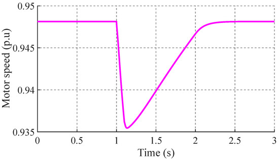
Figure 11.
Motor speed response.
Figure 12 shows the active power response of motor B after the delayed voltage recovery disturbance shown in Figure 8. The results of both the proposed model and the reference result of [18] indicate a reduction in active power from 0.948 p.u. to 0.45 p.u. during the voltage dip, which is consistent with the predicted behavior of induction motors [4,9,19]. It should be noted that the proposed model predicts the occurrence of a secondary active power peak at 1.1 s during the voltage recovery phase, which is not observed in the reference data. However, both models show a return to steady state at 1.2 s, confirming the stability of the system.
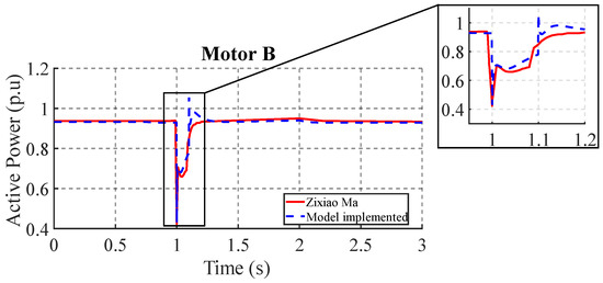
Figure 12.
Active power response in motor B.
Figure 13 plots the reactive power response of the motor after the voltage disturbance. The initial steady state reactive power was 0.68 p.u. After the voltage drop, the reactive power decreased to −0.7 p.u., indicating a significant change in the motor operating conditions. It is emphasized that the proposed model predicts a secondary reactive power pulse at 1.1 s, reaching 1.1 p.u., while the reference results [18] show a lower peak of 0.77 p.u.
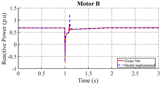
Figure 13.
Reactive power response in motor B.
Figure 12 and Figure 13 show an initial reduction in active power in the presence of a voltage drop. This coincides with the expected decrease in electromagnetic torque in the motor as mentioned [6]. Similarly, the active power shows an overshoot as the motor increases its rated speed. The reactive power response, characterized by a more pronounced peak, reflects the high magnetizing current demand of the motor during the transient [2].
Validation of Motor C
Figure 14 shows the active power response of motor C to the voltage perturbation show in Figure 8. Both the proposed and Zixiao Ma [18] models show similar steady-state responses. The magnitude of the steady-state active power is similar for both models (0.94 p.u.), indicating agreement in the mechanical loading of both models. Differences are observed in the transient response, in the second power pulse that occurs at 1.1 s. The proposed model has a higher impulse (1.2 p.u.) compared to Zixiao Ma’s model (1.02 p.u.).
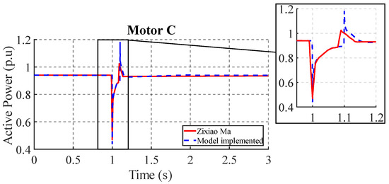
Figure 14.
Active power response in motor C.
Figure 15 shows the reactive power response of motor C to the voltage disturbance. Both the proposed and Zixiao Ma models show a similar response in the steady-state reactive power magnitude (0.68 p.u.). Some differences are observed in the transient response occurring at 1.1 s. The proposed model shows a more abrupt peak (1.35 p.u.) compared to the Zixiao Ma model (0.8 p.u.).
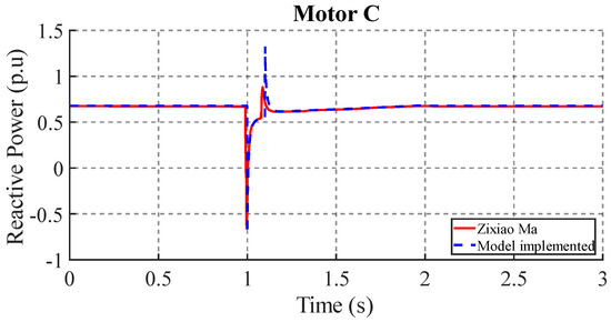
Figure 15.
Reactive power response in motor C.
A comparison with the results of [18] confirms that the proposed model adequately captures the behavior of induction motors under voltage disturbances. The small numerical discrepancies observed can be attributed to variations in the operating conditions considered in each study. The results obtained are consistent with electrical machine theory and validate the accuracy of the developed models.
3.2.2. Motor Load Variation
Figure 16 shows the reactive power response of motor A using the parameters in Table 3 under no-load conditions at a voltage disturbance of 75%. The proposed model and Kyle Stewart’s model [4] show similar behavior in the steady-state reactive power magnitude (0.7 p.u.), which indicates agreement in the representation of the motor load. Differences are observed in the transient response, especially in the magnitude of the reactive power pulses. The proposed model shows higher peaks, which could be due to the inclusion of the D and constants in Equation (14), which take into account mechanical losses and damping. These constants may introduce more damping into the system, which could explain the difference in the magnitude of the peaks.
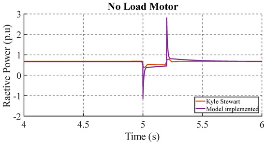
Figure 16.
Reactive power response in no-load motor.
Figure 17 shows a similar response between the two models for the reactive power of the motor at constant load. The proposed model presents a reactive power peak with a magnitude of 3.1 p.u., while the Kyle Stewart model was 1.2 p.u. This could be attributed to the inclusion of constants D and in the implemented model, which take into account mechanical losses and damping. The application of constant torque increases the reactive power demand of the motor, which explains the higher magnitude of the peaks compared to the unloaded motor.
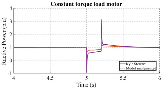
Figure 17.
Reactive power response in the motor with constant load.
A cross analysis of Figure 16 and Figure 17 shows the ability of the proposed model to accurately simulate the behavior of the induction motor under different load conditions. These differences suggest that the proposed model is able to more accurately capture the effects of load and mechanical losses on the dynamic behavior of the motor.
Comparing the results of the motor at no load (Figure 16) and at constant load (Figure 17), it is observed that the model captures the changes in the reactive power response due to the inclusion of the constants D and in the model. This inclusion is fundamental to explain the differences observed in the reactive power peaks, since it takes into account the mechanical losses and the damping of the motor.
3.2.3. Variation in Voltage Disturbance Magnitude
Figure 18 shows the response of the induction motor active power to different magnitudes of voltage drop. It is observed that as the magnitude of the voltage dip increases, the active power experiences a more substantial change and a longer recovery time. For an 85% drop, the power is significantly reduced, reaching a minimum value of approximately 0.4 p.u. and with a peak recovery of 1.05 p.u. that quickly stabilizes at 1.15 s. On the other hand, for a drop of 65%, the power is reduced to a lesser extent to 0.8 pu, and the peak recovery is 1.4 pu with a recovery time of 1.2 s. Finally, for a drop of 45%, a greater oscillation of the active power is observed, the peak recovery is greater than 2 p.u., and the recovery time reached was 1.4 seconds.
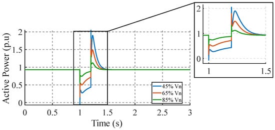
Figure 18.
Active power response with variation in voltage disturbance magnitude.
Figure 19 shows the reactive power response of the induction motor to different magnitudes of voltage disturbance. For an 85% drop, the reactive power peak reaches a maximum value of 1.2 p.u. and recovers quickly. For a 65% drop, the reactive power peak reaches a maximum value of 3.2 p.u. and reaches a steady state in 1.2 s. For a 45% drop, the peak reaches a value of 5 p.u., being the highest of the three cases, and the recovery time of 1.4 s is the longest.
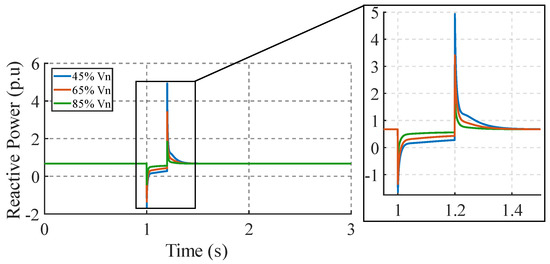
Figure 19.
Reactive power response with variation in voltage disturbance magnitude.
The speed of an induction motor is directly related to the frequency of the supply voltage and the number of poles. As the voltage decreases, the motor speed also decreases due to the reduction of magnetic flux in the air gap [24]. Figure 20 shows the response of the motor speed to different levels of voltage dips. For an 85% dip, the speed decreases to 352 rad/s, while for 65% and 45% dips, the speed decreases to 338 rad/s and 323 rad/s, respectively. These results confirm that voltage sags have a significant impact on motor performance, causing a reduction in speed and, in extreme cases, motor stalling.
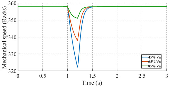
Figure 20.
Velocity response with variation in voltage disturbance magnitude.
The analysis of Figure 18, Figure 19 and Figure 20 shows the ability of the proposed model to accurately simulate the motor response under variations in the magnitude of the voltage disturbances, which makes it possible to evaluate the effect of the disturbances on key system variables such as active power, reactive power, and speed. These results demonstrate the sensitivity of the model to variations in the supply voltage and the importance of considering the magnitude of the disturbances when evaluating system performance.
4. Conclusions
This study implemented a detailed fifth-order mathematical model of a three-phase induction motor as a WECC load representation and validated its performance against models proposed in the literature. The methodology provided a step-by-step representation of the dynamic model of the motor in the direct and quadrature (dq) axes, which facilitated a better understanding of the transient and subtransient behavior under voltage perturbations. By simulating the induction motor model in MATLAB/Simulink and comparing it with alternative models, the accuracy and reliability of the proposed model was demonstrated.
The validation results showed that the model replicates the motor response to voltage dips and recovery. The transient reactive power peaks and the observed speed changes due to disturbances are consistent with established literature results, confirming the model’s ability to predict stability problems in systems with high induction motor penetration. The use of Type A, B, and C motor parameters, as well as variations in load and voltage disturbance magnitudes, highlighted the robustness of the model to various real-world scenarios.
These results highlight the impact of voltage dips on reactive power consumption, which can lead to motor lock-up and contribute to the problem of fault-induced delayed voltage recovery (FIDVR). This is particularly critical in scenarios where multiple three-phase induction motors are connected to the same load bus, as the cumulative effect of reactive power consumption affects voltage stability.
Despite its strengths, the model has limitations. It does not take into account the use of variable frequency drives and the implementation of automation and control systems that affect system dynamics. The lack of representation of overcurrent protection leads to limitations in the analysis of fault scenarios. These limitations suggest that future research should focus on extending the model to include a wider variety of components and control systems. Including models of variable frequency drives and protection systems would allow for a more realistic analysis of the behavior of modern electrical systems.
Despite these limitations, the proposed model demonstrates the ability to simulate the motor response to voltage disturbances and to analyze the stability of electrical systems with increasing motor loads. The results obtained can be used to design more robust protection and control systems.
Future work should focus on developing methodologies to identify the parameters of different types of motors, including laboratory tests to validate the model with real data, which would allow a more complete characterization of motor load dynamics in delayed voltage recovery studies, ensuring accuracy and reliability. Integration of this model, implemented in power system simulation software to analyze large networks, could allow its use in voltage stability studies.
Author Contributions
Conceptualization, K.L.-V., S.L.-E., J.P.M.-B., S.A.E.-M., C.A.V.-H., J.R.V.-M. and M.A.M.-C.; data curation, K.L.-V. and S.L.-E.; formal analysis, K.L.-V., S.L.-E., J.P.M.-B. and S.A.E.-M.; funding acquisition, K.L.-V., S.L.-E., J.P.M.-B., C.A.V.-H., J.R.V.-M. and M.A.M.-C.; investigation, K.L.-V., S.L.-E., J.P.M.-B. and S.A.E.-M.; methodology, K.L.-V., S.L.-E. and J.P.M.-B.; software, K.L.-V. and S.L.-E.; supervision, K.L.-V., S.L.-E. and J.P.M.-B.; writing—original draft, K.L.-V., S.L.-E. and J.P.M.-B.; writing—review & editing, K.L.-V., S.L.-E., J.P.M.-B., C.A.V.-H., J.R.V.-M. and M.A.M.-C. All authors have read and agreed to the published version of the manuscript.
Funding
This research received no external funding.
Data Availability Statement
The original contributions presented in the study are included in the article, further inquiries can be directed to the corresponding author.
Conflicts of Interest
The authors declare no conflict of interest.
Abbreviations
The following abbreviations are used in this manuscript:
| FIDVR | Fault-induced delayed voltage recovery. |
| GE PSLE | General electric power system load flow. |
| PSSE | Power system simulation for engineering. |
| Quasi-AC | The simple steady-state model of the motor. |
| WECC | Western Electricity Coordinating Council. |
| ZIP | Polynomial model of constant impedance, constant current, and constant power. |
| ZIP + IM | ZIP model in parallel to induction motor. |
Appendix A. Script MATLAB. Determination of (, , , , and )
| Listing A1. MATLAB code for the determination of , , and |
 |
References
- Tan, B.; Zhao, J.; Duan, N. Amortized Bayesian Parameter Estimation Approach for WECC Composite Load Model. IEEE Trans. Power Syst. 2023, 39, 1517–1529. [Google Scholar] [CrossRef]
- Taylor, C.W. Voltage Stability. Power System Voltage; Mcgraw-Hill: New York, NY, USA, 1994; pp. 27–32. [Google Scholar]
- Lee, Y.; Song, H. Multi-Phase Under Voltage Load Shedding Scheme for Preventing Delayed Voltage Recovery by Induction Motor Power Consumption Characteristics. Appl. Sci. 2018, 8, 1115. [Google Scholar] [CrossRef]
- Stewart, K.; Taylor, G.A.; Halpin, S.M. Motor Load Models for Fault-Induced Delayed Voltage Recovery Studies in Bulk Transmission Systems. In Proceedings of the 2023 IEEE International Conference on Environment and Electrical Engineering and 2023 IEEE Industrial and Commercial Power Systems Europe, Madrid, Spain, 6–9 June 2023; pp. 1–5. [Google Scholar] [CrossRef]
- Khazeiynasab, S.R.; Zhao, J.; Duan, N. WECC Composite Load Model Parameter Identification Using Deep Learning Approach. In Proceedings of the 2022 IEEE Power & Energy Society General Meeting (PESGM), Denver, CO, USA, 17–21 July 2022; pp. 1–5. [Google Scholar] [CrossRef]
- Kundur, P. Power System Stability and Control; CRC Press: Boca Raton, FL, USA, 1994. [Google Scholar]
- McCormick, K. Distribution Level Composite Load Modeling. Master’s Thesis, University of Pittsburgh, Pittsburgh, PA, USA, 2023. [Google Scholar]
- Liao, W.; Zhang, Y.; Zhou, R. Analytical method to calculate transient responses of induction motor load. IET Gener. Transm. Distrib. 2020, 14, 3221–3229. [Google Scholar] [CrossRef]
- Rahmani, S.; Rezaei-Zare, A. Prediction of System Voltage Recovery due to Single Phase Induction Motor Stall Using Machine Learning Techniques. In Proceedings of the 2019 IEEE Workshop on Electrical Machines Design, Control and Diagnosis (WEMDCD), Athens, Greece, 22–23 April 2019; Volume 1, pp. 128–134. [Google Scholar] [CrossRef]
- Zhang, K.; Zhu, H.; Guo, S. Dependency Analysis and Improved Parameter Estimation for Dynamic Composite Load Modeling. IEEE Trans. Power Syst. 2017, 32, 3287–3297. [Google Scholar] [CrossRef]
- IEEE Guide for Load Modeling and Simulations for Power Systems; The Institute of Electrical and Electronics Engineers, Inc.: New York, NY, USA, 2022; Available online: https://ieeexplore.ieee.org/document/9905546 (accessed on 9 February 2025).
- Yamashita, K.; Martinez Villanueva, S.; Djokic, S.; Ma, J.; Gaikwad, A.; Milanović, J. CIGRE SC C4 2012 Hakodate Colloquium Overview of Existing Methodologies for Load Model Development. In Proceedings of the Coloquio CIGRE SC C4 en Japón, Hakodate, Japan, 11–12 October 2012. [Google Scholar]
- Kosterev, D.N.; Taylor, C.W.; Mittelstadt, W.A. Model validation for the August 10, 1996 WSCC system outage. IEEE Trans. Power Syst. 1999, 14, 967–979. [Google Scholar] [CrossRef]
- Ma, Z.; Cui, B.; Wang, Z.; Zhao, D. Parameter Reduction of Composite Load Model Using Active Subspace Method. IEEE Trans. Power Syst. 2021, 36, 5441–5452. [Google Scholar] [CrossRef]
- Xie, J.; Ma, Z.; Dehghanpour, K.; Wang, Z.; Wang, Y.; Diao, R.; Shi, D. Imitation and Transfer Q-Learning-Based Parameter Identification for Composite Load Modeling. IEEE Trans. Smart Grid 2021, 12, 1674–1684. [Google Scholar] [CrossRef]
- Arif, A.; Wang, Z.; Wang, J.; Mather, B.; Bashualdo, H.; Zhao, D. Load Modeling—A Review. IEEE Trans. Smart Grid 2018, 9, 5986–5999. [Google Scholar] [CrossRef]
- Wang, Z.; Bu, F.; Ma, Z.; Xiang, Y. Data-Driven and Machine Learning-Based Load Modeling. 2021. Available online: https://documents.pserc.wisc.edu/documents/publications/reports/2021_reports/S_84G_Final_Report.pdf (accessed on 9 February 2025).
- Ma, Z.; Wang, Z.; Wang, Y.; Diao, R.; Shi, D. Mathematical Representation of WECC Composite Load Model. J. Mod. Power Syst. Clean Energy 2020, 8, 1015–1023. [Google Scholar] [CrossRef]
- Huang, Q.; Huang, R.; Palmer, B.J.; Liu, Y.; Jin, S.; Diao, R.; Chen, Y.; Zhang, Y. A generic modeling and development approach for WECC composite load model. Electr. Power Syst. Res. 2019, 172, 1–10. [Google Scholar] [CrossRef]
- Bu, F.; Ma, Z.; Yuan, Y.; Wang, Z. WECC Composite Load Model Parameter Identification Using Evolutionary Deep Reinforcement Learning. IEEE Trans. Smart Grid 2020, 11, 5407–5417. [Google Scholar] [CrossRef]
- Liu, Y.; Zhang, Y.; Huang, Q.; Kundu, S.; Tang, Y.; James, D.; Etingov, P.; Mitra, B.; Chassin, D.P. Impact of Building-Level Motor Protection on Power System Transient Behaviors. In Proceedings of the 2018 IEEE Power & Energy Society General Meeting (PESGM), Portland, OR, USA, 5–10 August 2018; pp. 1–5. [Google Scholar] [CrossRef]
- WECC. WECC Composite Load Model Specification; WECC: Salt Lake City, UT, USA, 2021. [Google Scholar]
- Aree, P. Third-Order Polar-Coordinate Model of Induction Motor Load. In Proceedings of the 2023 9th International Conference on Engineering, Applied Sciences, and Technology (ICEAST), Vientiane, Laos, 1–4 June 2023; pp. 140–143. [Google Scholar] [CrossRef]
- Chapman, S.J. Maquinas Electricas, 5th ed.; Mc Graw Hill: New York, NY, USA, 2012; pp. 231–299. [Google Scholar]
- Krause, T.R.K.P.C. Introduction to Modern Analysis of Electric Machines and Drive; Wiley-IEEE Press: Hoboken, NJ, USA, 2022. [Google Scholar]
- Chen, Y.; Wu, H.; Shen, Y.; Meng, X.; Ju, P. A Fast Parameter Identification Method for Composite Load Model Based on Jumping and Steady-State Points of Measured Data. IEEE Access 2022, 10, 97665–97676. [Google Scholar] [CrossRef]
- Huang, Q.; Huang, R.; Palmer, B.J.; Liu, Y.; Jin, S.; Diao, R.; Chen, Y.; Zhang, Y. A Reference Implementation of WECC Composite Load Model in Matlab and GridPACK. arXiv 2017, arXiv:1708.00939. [Google Scholar] [CrossRef]
- Sharawy, M.; Shaltout, A.A.; Youssef, O.E.S.M.; Al-Ahmar, M.A.; Abdel-Rahim, N.; Sutikno, T. Maximum allowable hp rating of 3-phase induction motor fed through a stand-alone constant V/f controlled DFIG via RSC. Bull. Electr. Eng. Inform. 2024, 13, 832–844. [Google Scholar] [CrossRef]
- Rasheduzzaman, M.; Mueller, J.A.; Kimball, J.W. An Accurate Small-Signal Model of Inverter- Dominated Islanded Microgrids Using dq Reference Frame. IEEE J. Emerg. Sel. Top. Power Electron. 2014, 2, 1070–1080. [Google Scholar] [CrossRef]
- NERC. Technical Reference Document Dynamic Load Modeling; NERC: Atlanta, GA, USA, 2016. [Google Scholar]
- Hernández, G.; Jonathan, M.U.P.J.; Martínez, O.V. Determinación de la Constante de Inercia de Máquinas Síncronas de Laboratorio. 2010. Available online: https://tesis.ipn.mx/jspui/bitstream/123456789/8554/1/90.pdf (accessed on 9 February 2025).
- Belbali, A.; Makhloufi, S.; Kadri, A.; Abdallah, L.; Seddik, Z. Mathematical Modeling of a Three-Phase Induction Motor; IntechOpen: London, UK, 2023; Chapter 7. [Google Scholar] [CrossRef]
- Sengamalai, U.; Anbazhagan, G.; Thentral, T.M.T.; Vishnuram, P.; Khurshaid, T.; Kamel, S. Three Phase Induction Motor Drive: A Systematic Review on Dynamic Modeling, Parameter Estimation, and Control Schemes. Energies 2022, 15, 8260. [Google Scholar] [CrossRef]
Disclaimer/Publisher’s Note: The statements, opinions and data contained in all publications are solely those of the individual author(s) and contributor(s) and not of MDPI and/or the editor(s). MDPI and/or the editor(s) disclaim responsibility for any injury to people or property resulting from any ideas, methods, instructions or products referred to in the content. |
© 2025 by the authors. Licensee MDPI, Basel, Switzerland. This article is an open access article distributed under the terms and conditions of the Creative Commons Attribution (CC BY) license (https://creativecommons.org/licenses/by/4.0/).