Reduction in the Electromagnetic Interference Generated by AC Overhead Power Lines on Buried Metallic Pipelines with Screening Conductors

Abstract

This paper presents a numerical study on the reduction in the voltage and current induced on a $13.5$ km buried metallic pipeline by an overhead power line. The mitigation effectiveness of different configurations and cross-section shapes of screening conductors is computed by means of a methodology that combines a 2D Finite Element Analysis with circuital analysis. A $35.72$% reduction of the maximum induced voltage is obtained when 4 cylindrical steel screening conductors with 8 $\mathrm{mm}$ radius are buried $0.25$ $\mathrm{m}$ below the soil surface, along the pipeline path. The maximum induced pipeline current is reduced by $26.98$%. A parametric study is also performed, to assess the influence of the per-unit-length admittance to earth of the screening conductors on the mitigation efficacy. The results show that screening conductors may help in reducing the inductive coupling between overhead power lines and buried metallic pipelines, and that the assumption of perfectly insulated screening conductors leads to an underestimation of the produced mitigation effect.

1. Introduction

Metallic pipelines located in the proximity of power lines can be exposed to electromagnetic interference during both normal operating conditions and faults of the latter [1,2,3]. Because of the high cost of right-of-ways, it is in fact unavoidable that the pipelines share the same corridor with high-voltage AC (HVAC) power lines [4,5,6]. It is then likely that electromagnetic interference may occur, where the source is constituted by the HVAC power line and the victim by the metallic buried pipeline [7,8,9]. In general, this electromagnetic interference consists of inductive, capacitive and conductive contributions [10] which can be studied and assessed with three different coupling mechanisms. For underground metallic pipelines, the capacitive coupling (also called electrostatic coupling) is not particularly significant as the earth provides a quite efficient screen to the electrostatic field generated by the difference of potential between the power line and the pipeline [11]. The conductive coupling is noteworthy during fault conditions, where the currents in the power line may reach much higher values than in the steady-state condition and thus the pipeline coating may be subject to a larger potential difference between the pipeline and the surrounding soil [12,13,14]. For an overhead power line in sinusoidal steady-state, the most significant coupling mechanism of the three above mentioned is then the inductive coupling mechanism, which is due to the magnetic field generated by the power line currents [15,16]. The inductive coupling between the power line and the pipeline results in an induced voltage in the pipeline that may increase the risks for electrochemical corrosion [17,18], damage to insulation [19,20] and electrical shock [21]. In order to reduce the electromagnetic interference between source and victim, the most practical solution consists in worsening the electromagnetic coupling. The use of screening conductors buried in the soil above the metallic pipelines appears then as a feasible solution to attenuate the voltage generated on the pipeline by inductive coupling [22].

In previous works [23], it has been shown that the assessment of simple geometries such as those represented by the cross section of mitigation wires (MWs) with the Quasi-3d methodology yields results which are in good agreement with those obtained in [4], where a widely used analytical methodology is illustrated. Compared to other analytical methods, the developed numerical methodology allows an accurate physical description of complex geometries, too. With the developed method, no limitation on the number of conductors (either buried or overhead) is introduced; moreover, the soil electrical resistivity can be modelled as an analytical function of space.

The developed methodology has been employed by the authors in [24] to study the influence of the screening conductor’s shape and magnetic properties on their mitigation efficacy. In this work, the same technique is applied to a different pipeline–power line routing, focusing on the effects produced by different values of the screening conductors’ admittance to earth on the mitigation efficacy yielded by the screening conductors.

This paper is organised as follows: Section 2 describes the proposed hybrid methodology (composed of Finite Element Analysis and circuit analysis); the results are presented in Section 3, where the induced pipe-to-soil voltage and longitudinal pipe current are obtained for different configurations of screening conductors, and discussed in Section 4.

2. Mathematical Model

The numerical study presented in this work is conducted using a computer code developed by the authors, implementing the methodology described in [23]. In particular, the main feature of the developed approach lies in the combination of 2D Finite Element Analysis (FEA) and circuital analysis; this allows one to study the electromagnetic interference induced on metallic structures that can extend over several kilometers following non-straight paths without having to rely on 3D FEA, that would entail a prohibitive computational load. As depicted in Figure 1, a corridor comprising a power line, a pipeline and other conductors (such as mitigation wires) is subdivided in a certain number of 2D sections. Hence, each section typically includes one or more HVAC overhead power lines, one or more metallic pipelines buried in the soil and other additional conductors, such as mitigation wires. Each section is discretized and subsequently simulated via 2D FEA. The given section represents the specific characteristics of the studied configuration at a given position along corridor. Hence, the relative positioning between the considered conductors and the electric characteristics of the soil as well as the metallic conductors can be different from section to section. The influence on the obtained accuracy exerted by the number of sections in which the corridor is subdivided has been assessed in [25]. In this respect, it should be highlighted that the considered sections are not physically independent one from the other. As anticipated, a circuital methodology is employed to enforce the physical interconnection between different corridor sections. That is, for each considered section of the corridor, FEA is used to extract the local physical characteristics in terms of voltages and currents. These are subsequently fed into an equivalent electric network in the form of multiport circuital components (one for each corridor section). The obtained multiport components are finally embedded into an electrical circuit, equivalent to the considered corridor.

2.1. Finite Element Formulation

The developed finite element solver is employed to study each section of the corridor, by solving a 2D quasi-magnetostatic problem. The employment of such formulation implies that only the conduction current contributions to the magnetic field is considered, neglecting the displacement current. Furthermore—since the solver is employed to study the effects of HVAC power lines in standard operating conditions—the considered system is assumed to work in sinusoidal steady-state. Moreover, the modeled materials are assumed to be linear and isotropic. This is also applied to any ferromagnetic materials, given that the magnetic field intensities produced by typical power line current values are markedly below [24] saturation. For each section of the discretized corridor, the current density in all the conductors is assumed to flow perpendicularly to the considered plane. Hence, assuming that the power line is directed along $\widehat{z}$, then $\overrightarrow{J}=J_z(x,y,t)\widehat{z}$ and a magnetic vector potential can be defined for the magnetic field, such that $\overrightarrow{B}=\nabla \times \overrightarrow{A}$, and $\overrightarrow{A}=A_z(x,y,t)\widehat{z}$. These physical assumptions (the reader is referred to [26] for a more in-depth discussion) allow the attainment of a time-independent complex expression for the magnetic potential vector diffusion equation:

$$-\nabla ·\left(\frac{1}{\mu }\nabla \underline{A_z}\right)=\underline{J_{0,z}}-j\omega \sigma \underline{A_z}.$$

(1)

In the former expression, $\mu$ is the magnetic permeability, while $\underline{J_{0,z}}$ and $\underline{A_z}$ are the phasors associated with the current enforced by voltages along the corridor and the magnetic vector potential, respectively. The discretization of Equation (1) with a finite element approach leads to a linear systems [27], yielding the values of $\underline{A_z}$ on the nodes of the discretized domain:

$$\left[\underline{K}\right]\left\{{\underline{A}}_z\right\}=\{\underline{f}\}.$$

(2)

The right-hand side of Equation (2) includes the term $\underline{J_{0,z}}$ in Equation (1) and the boundary conditions for the considered quasi-magnetostatic problem. Hence, Equation (2) expresses the relation between the impressed current densities (i.e., $\underline{J_{0,z}}$), acting as forcing terms for the differential problem, and the magnetic vector potential distribution in the given section of the corridor. Hence, the finite element approach is employed to take into account the physical contribution provided by electric fields (and hence current densities) in the direction perpendicular to each section of the corridor, i.e., along the power line path. The aforementioned circuital approach is instead employed to constrain the forcing terms ($\underline{J_{0,z}}$), such that the effects of electric fields that are not directed along $\widehat{z}$—that cannot be directly modeled with the employed 2D finite element approach—are addressed. This allows one to take into account any connection between the metallic conductors and between a conductor and the soil, as well as interactions between the 2D sections employed to subdivide the corridor.

2.2. Equivalent Circuit

As anticipated in the former sections, a generic corridor including a nonparallel pipeline–power line routing is approximated by a number of 2D sections of the corridor. In this way, the routing is approximated by a number of straight segments, where each segment correspond to a single 2D section. FEA is then performed on each segment (hence section), to derive the relation between the forcing terms and the induced currents through each conductor. The subsequently obtained current density $\underline{J_z}$ is integrated over the cross section of each conductor, yielding the corresponding electric current $\underline{I_h}$. Hence, a characteristic matrix $\left[\underline{M}\right]$ can be defined for each section, representing the linear relation between the forcing terms and the currents in each conductor:

$$\left\{\underline{I}\right\}=\left[\underline{M}\right]\{\underline{J_{z,0}}\}.$$

(3)

The term $\left\{\underline{I}\right\}$ in Equation (3) represents the currents $\underline{I_1},\underline{I_2},\cdots ,\underline{I_n}$ flowing through the n conductors of a given corridor section, while $\{\underline{J_{z,0}}\}$ represents the corresponding array of impressed current densities. The generic entry ${\underline{m}}_{h,k}$ of $\left[\underline{M}\right]$ corresponds to the current $\underline{I_h}$ induced on the hth conductor of the section, when a unit current density $\underline{J_{0,z,k}}$ is enforced on the kth one. Hence, in order to compute $\left[\underline{M}\right]$ for a given section including n conductors, a corresponding number of instances of the FEA solver must be invoked. Moreover, since $\underline{J_{z,0,k}}=\frac{{\sigma }_k}{L_s}\underline{V_k}$, a characteristic matrix can also be regarded as the constitutive relation of an n-port electric component. In this way, the FEA of the different sections used to discretize the routing yield a corresponding number of n-port components. The latter are then inserted into the cells of an equivalent electrical network, which consequently include the information extracted via FEA. Moreover, as anticipated, each cell may contain admittances, which represent the connections existing between metallic conductors, or between a conductor and the soil. Finally, the solution of the equivalent network—yielding the currents and voltages in the considered conductors at each section of the corridor—can be obtained with any circuital analysis technique. The code developed by the authors uses the tableau analysis methodology, as detailed in [23].

3. Results

In this section, the described Quasi-3D approach is employed to assess the mitigation effectiveness associated with different shapes and arrangements of a set of screening conductors. These are buried in the soil above the pipeline, and follow its path along the route depicted in Figure 1. Each numbered mark along the pipeline path in Figure 1 corresponds to a specific characteristic matrix yielded by a 2D FEM simulation of the corresponding cross section of the routing.

Figure 2 shows the geometric characteristics of the considered power line, that is, the positions of the power wires and Overhead Ground Wire (OGW), as well as the burial depth and relative position of the pipeline and four different mitigation wires. The x coordinate of the pipeline conductor is reported as an interval, corresponding to the position of the pipeline (and mitigation wires) with respect to the power line center for each of the 34 cross-sections of the routing marked in Figure 1. In [28], the influence on the mitigation effectiveness of the number and burial depth of the screening conductors has been assessed. As reported in Figure 2, a constant burial depth of $0.25\mathrm{m}$ was used in this work for the sake of practicality.

Table 1. Geometrical and electrical data.

Quantity	Value	Units
${\underline{I}}_I$—Phase I	$1000\underline{/0°}$	$\mathrm{A}$
${\underline{I}}_{II}$—Phase II	$1000\underline{/120°}$	$\mathrm{A}$
${\underline{I}}_{III}$—Phase III	$1000\underline{/-120°}$	$\mathrm{A}$
${\sigma }_{soil}$	1 × 10−3	$\mathrm{S}\mathrm{m}$−1
${\sigma }_{pipe}$	5.5 × 106	$\mathrm{S}\mathrm{m}$−1
${\sigma }_{OGW}$	3.77 × 107	$\mathrm{S}\mathrm{m}$−1
${\sigma }_{MW}$	5.5 × 106	$\mathrm{S}\mathrm{m}$−1
Pipe external radius	0.4	$\mathrm{m}$
Pipe internal radius	0.375	$\mathrm{m}$
OGW radius	6 × 10−3	$\mathrm{m}$
${\mu }_{r,soil}$	1	−
${\mu }_{r,pipe}$	250	−
${\mu }_{r,OGW}$	1	−
${\mu }_{r,MW}$	1	−
${\underline{y}}_{pipe-soil}^{\prime }$	3 × 10−4 + 9 × 10−6i	$\mathrm{S}\mathrm{m}$−1
${\underline{z}}_{pipe-soil}$	3	$\mathsf{\Omega }$
${\underline{y}}_{ogw-soil}^{\prime }$	1 × 10−3	$\mathrm{S}\mathrm{m}$−1
${\underline{z}}_{ogw-soil}$	1	$\mathsf{\Omega }$

summarizes the main electrical and geometrical information on the considered physical configuration. The quantity ${\underline{y}}_{pipe-soil}^{\prime }$ is the per-unit-length (p.u.l.) admittance to earth of the power line, which has been computed with the expression recommended in [4], assuming a 7 mm thick pipeline coating, with a resistivity of $\rho =$ $6\times {10}^5$ $\mathrm{\Omega }$$\mathrm{m}$ and ${ϵ}_r=2$. In addition, in Table 1, ${\underline{z}}_{pipe-soil}$ represents the earthing impedance of the pipeline at both ends of the considered corridor. The value for the OGW admittance to soil (${\underline{y}}_{ogw-s}^{\prime }$) was obtained assuming that a power tower is installed every 100 $\mathrm{m}$ of the power line, and that the series of every power tower and its grounding system has a resistance of $10\mathrm{\Omega }$ [29,30], giving ${\underline{Y}}_{tower}=0.1\mathrm{S}$. Consequently, the power tower admittance-to-soil is then distributed over 100 $\mathrm{m}$, yielding the reported per-unit-length (p.u.l.) value. In [24] the mitigation wires were assumed to be perfectly earthed at both ends of the domain (${\underline{z}}_{MW}=0$), and perfectly insulated from the soil within the routing (${\underline{y}}_{MW-s}^{\prime }=0$), for the sake of simplicity. In this work, two other additional values for ${\underline{y}}_{MW-s}^{\prime }$ are considered together with ${\underline{y}}_{MW-s}^{\prime }=0$. These are ${\underline{y}}_{MW-s}^{\prime }=1.8\times {10}^{-3}\mathrm{S}/\mathrm{m}$, selected according to [31] and ${\underline{y}}_{MW-s}^{\prime }=\infty$.

3.1. Induced Current and Voltage in Absence of Mitigation Measures

In order to provide a reference case for the evaluation of different mitigation techniques performed in the next sections, the configuration described in the previous paragraph is first assessed without any mitigation device. Figure 3 shows the magnitudes of the obtained longitudinal pipeline current $I_{pipe}$ and pipeline-to-soil voltage $V_{pipe-soil}$ along the length of exposure, yielded by the network analysis. It is worth highlighting that—even if the term network analysis is used for the sake of conciseness—the tableau analysis is carried out using physical information extracted through finite element analysis of the discretised domain, as described in the previous section. The obtained results show that both the induced voltage-to-soil and current may reach considerable values, requiring the employment of mitigation means [32].

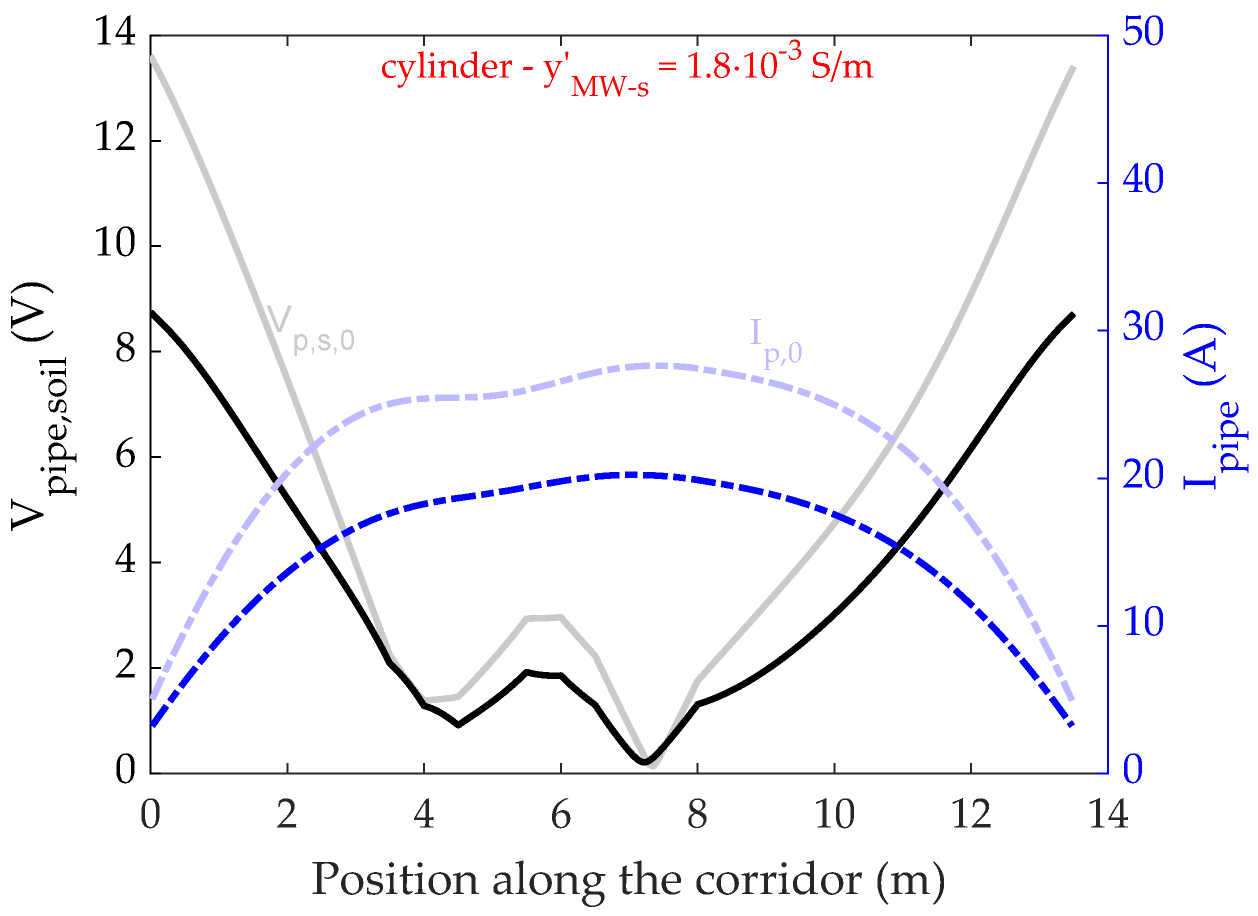
3.2. Cylindrical Mitigation Wires

In this test, four cylindrical mitigation wires are added to the same configuration described in Section 3.1. The wires are assumed to be made out of steel (${\sigma }_{MW}=$ $5.5\times {10}^6$ $\mathrm{S}{\mathrm{m}}^{-1}$), and with a radius of 8 $\mathrm{m}$$\mathrm{m}$. Figure 4 shows the obtained current and voltage profiles when the cylindrical mitigation wires are employed. This plot refers to a p.u.l. admittance ${\underline{y}}_{MW-s}^{\prime }=1.8\times {10}^{-3}$ S/m. Unless otherwise indicated, this value for the p.u.l. admittance to soil is retained for the results presented in this section.

The unmitigated voltage and current profiles of Figure 3 are reported for the sake of comparison, and are marked as $V_{p,s,0}$ and $I_{p,0}$, respectively.

3.3. Square Mitigation Wires

The aim of this second test is to assess the influence of the mitigation wire cross-section shape on the mitigation rate. The simulation described in the previous section is performed assuming that the mitigation wires have a square shape. Each side of the square cross-section has a length of $14.18$ $\mathrm{m}$$\mathrm{m}$, so that its cross-section area is approximately equal to the one of the cylindrical wires with 8 $\mathrm{m}$$\mathrm{m}$ radius employed in Section 3.2. The obtained profiles of pipe-to-soil voltage and pipeline current are shown in Figure 5 and compared to the unmitigated results.

The current density distribution obtained via the performed 2d FEA is shown in Figure 2 for $M{W}_a$ (with the naming convention employed in Figure 2). The figure refers to the 6th among the 34 cross-sections of the routing summarized in Figure 1, i.e., when the pipeline is located 3 $\mathrm{m}$ the right of the power-line centre.

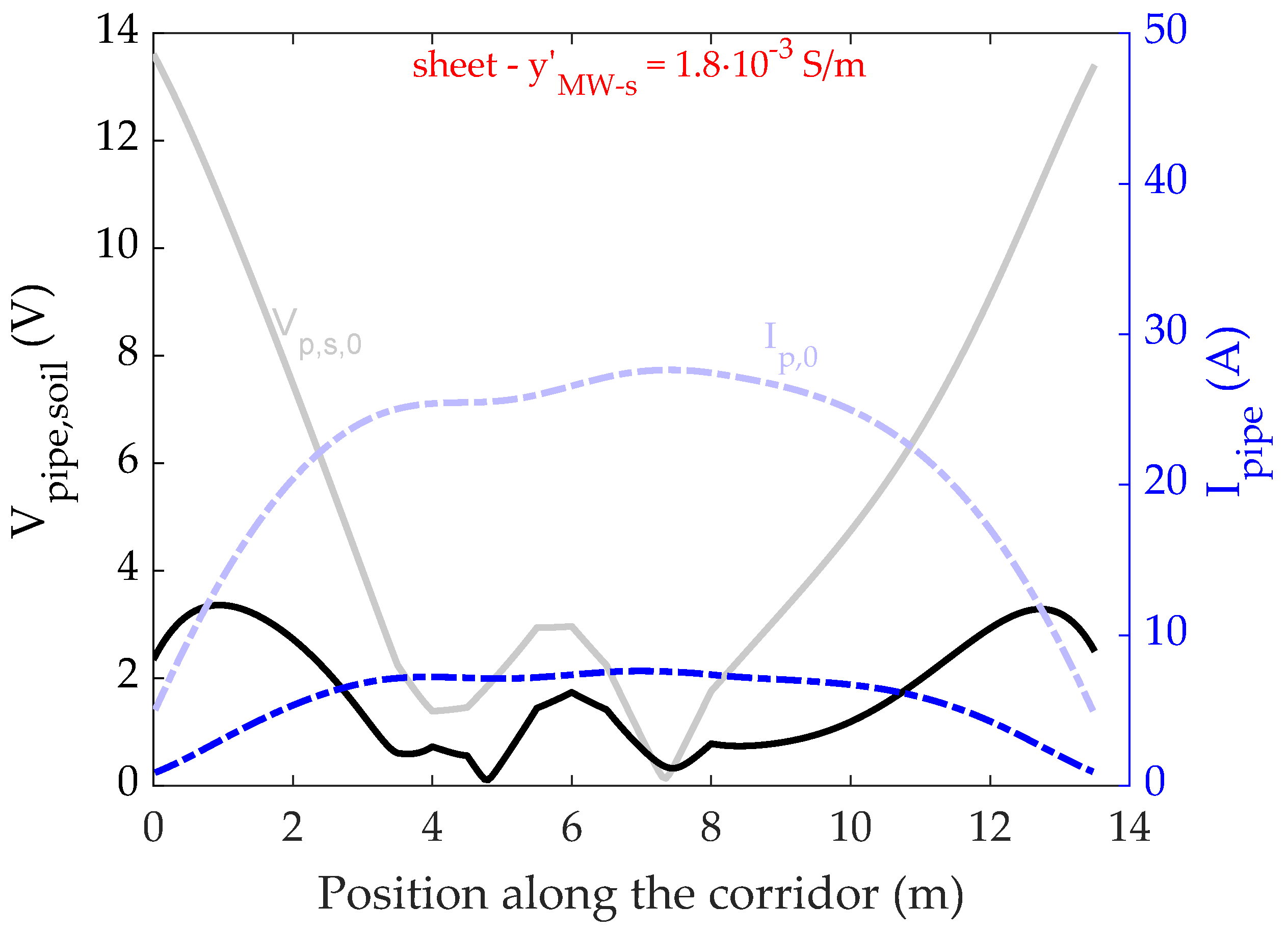
3.4. Sheet Mitigation Conductor

The simulations described in the previous sections are repeated considering a single large rectangular screening conductor for the four cylindrical and squared mitigation wires. This steel sheet has a width of $3.2$ $\mathrm{m}$ (equal to the distance between $M{W}_a$ and $M{W}_d$ in Figure 2). The thickness of the mitigation sheet is 8 $\mathrm{m}$$\mathrm{m}$, i.e., equal to the radius of the cylindrical mitigation wires of Section 3.2. The rationale behind this test is to provide a limit case, representative of the maximum mitigation effect that can be achieved for a given material and available horizontal span of the mitigation conductors. Figure 6 shows the obtained voltage-to-soil and current on the pipeline, with and without the mitigating steel sheet. Again, in this plot a p.u.l. admittance to soil ${\underline{y}}_{MW-s}^{\prime }=1.8\times {10}^{-3}\mathrm{S}/\mathrm{m}$ was chosen for the sheet screening conductor.

4. Discussion

In this section, the results of the test cases presented in Section 3 are discussed. Setting ${\underline{y}}_{MW-s}^{\prime }=0$ as in [24] corresponds to assuming that the mitigation wires are perfectly insulated from the surrounding soil. Conversely, ${\underline{y}}_{MW-s}^{\prime }=\infty$ means that the mitigation wires are perfectly earthed at each section of the employed electrical equivalent network. The obtained results are summarized in

Table 2. Summary of maximum pipe-to-soil voltage and pipeline current for the four different described configurations.

	I—Unmitigated	II—Cylinder	III—Square	IV—Sheet
$max\left(V_{p,s}\right)\left[\mathrm{V}\right]$	13.61	8.75	8.74	3.36
$max\left(I_p\right)\left[\mathrm{A}\right]$	27.63	20.23	20.21	7.62

,

Table 3. Voltage mitigation rate yielded by different values of the mitigation wire p.u.l. admittance to earth ${\underline{y}}_{MW-s}^{\prime }$.

${\underline{\mathit{y}}}_{\mathbf{MW}-\mathit{s}}^{\prime }\left(\mathbf{S}/\mathbf{m}\right)$	Cylinder—MRV (%)	Square—MRV (%)	Sheet—SMRV (%)
0	33.56	33.56	86.16
∞	35.42	35.49	78.71
$1.8\times {10}^{-3}$	35.72	35.78	82.73

and

Table 4. Current mitigation rate yielded by different values of the mitigation wire p.u.l. admittance to earth ${\underline{y}}_{MW-s}^{\prime }$.

${\underline{\mathit{y}}}_{\mathbf{MW}-\mathit{s}}^{\prime }\left(\mathbf{S}/\mathbf{m}\right)$	Cylinder—MRI (%)	Square—MRI (%)	Sheet—MRI (%)
0	26.10	26.15	65.09
∞	27.04	27.12	71.39
$1.8\times {10}^{-3}$	26.98	27.04	72.59

.

4.1. Induced Current and Voltage in Absence of Mitigation Measures

As one can see from Figure 3, a dual behavior can be observed in the induced current and voltage profiles, i.e, the zones with large current values correspond to low voltages-to-soil, and vice versa. This can be explained considering that $V_{pipe-soil}$ is proportional to the current flowing through the pipeline coating rather than $I_{pipe}$, which flows in the direction parallel to the pipeline path. The maximum values of the pipe-to-soil voltage and pipeline current are $V_{pipe-soil}=13.61$ V and $I_{pipe}=27.63$ A, respectively (see Table 2).

4.2. Cylindrical Mitigation Wires

As discussed in [33], the mitigation wires deviate the magnetic field lines produced by the HVAC overhead power line, exerting a shadowing effect on the underlying pipeline. The maximum values of the pipe-to-soil voltage and pipeline current are $V_{pipe-soil}=8.75$ V and $I_{pipe}=20.23$ A, respectively (see Table 2). Indeed, as can be observed in Figure 4, a marked reduction in both the induced voltage and current is obtained with the addition of the mitigation wires. The mitigation rate will be used here onwards to provide a quantitative description of the obtained mitigation efficacy. Considering, e.g., the induced pipeline-to-soil voltage, the voltage mitigation rate ($M{R}_V$) is defined as:

$$M{R}_V=\left(1-\frac{max\left(V_{p-s}\right)}{max\left(V_{pipe,0}\right)}\right)·100,$$

(4)

where $max\left(V_{p-s,0}\right)$ is the maximum pipe-to-soil voltage value along the corridor, when no mitigation means are considered.

For the present case, the achieved voltage and current mitigation rates are reported in Table 3 and Table 4 for the considered p.u.l. values of the mitigation wire to soil admittance. As regards voltage mitigation rates, they range from $M{R}_V=33.56$% to $M{R}_V=35.72$% for ${\underline{y}}_{MW}^{\prime }=0$ and ${\underline{y}}_{MW}^{\prime }=1.8\times {10}^{-3}$, respectively. The current mitigation rates range from $M{R}_I=26.20$% to $M{R}_I=27.04$% for ${\underline{y}}_{MW}^{\prime }=0$ and ${\underline{y}}_{MW}^{\prime }=\infty$, respectively.

4.3. Square Mitigation Wires

The obtained voltage and current profiles depicted in Figure 5 show that, in analogy with the cylindrical wires test, a reduction in both the induced voltage and current is achieved. The maximum values of the pipe-to-soil voltage and pipeline current are $V_{pipe-soil}=8.74$ V and $I_{pipe}=20.21$ A, respectively (see Table 2). These values are very close to those obtained with the cylindrical mitigation wires. Correspondingly, the voltage and current mitigation rates are similar; the former range from $M{R}_V=33.56$% to $M{R}_V=35.78$% (obtained for ${\underline{y}}_{MW}^{\prime }=0$ and ${\underline{y}}_{MW}^{\prime }=1.8\times {10}^{-3}$, respectively), whereas the latter range from $M{R}_I=26.15$% to $M{R}_I=27.12$% (obtained for ${\underline{y}}_{MW}^{\prime }=0$ and ${\underline{y}}_{MW}^{\prime }=\infty$, respectively). This is a somewhat expected result, since the cross section area of the two different kind of mitigation wires is the same. In addition, since the wires are assumed to be made out of steel, the magnetic field penetration depth is larger than their characteristic size. For this reason, the current density distribution is approximatively uniform within the wires, as can be verified in the field map shown in Figure 7.

4.4. Sheet Mitigation Conductor

As one can see from Table 3 and Table 4, a marked reduction in the induced voltage is achieved with respect to the unmitigated reference case, for any value of the mitigation wire-to-soil admittance. In fact, the conductive sheet produces the maximum mitigation effect that can be achieved for a given material and available horizontal span of the mitigation conductors.

The 2D spatial current density distribution in the appurtenances of the pipeline and the mitigating steel sheet can be observed in Figure 8. The plot highlights the shadowing effect produced by the current density induced in the mitigation sheet by the magnetic field produced by the power line.

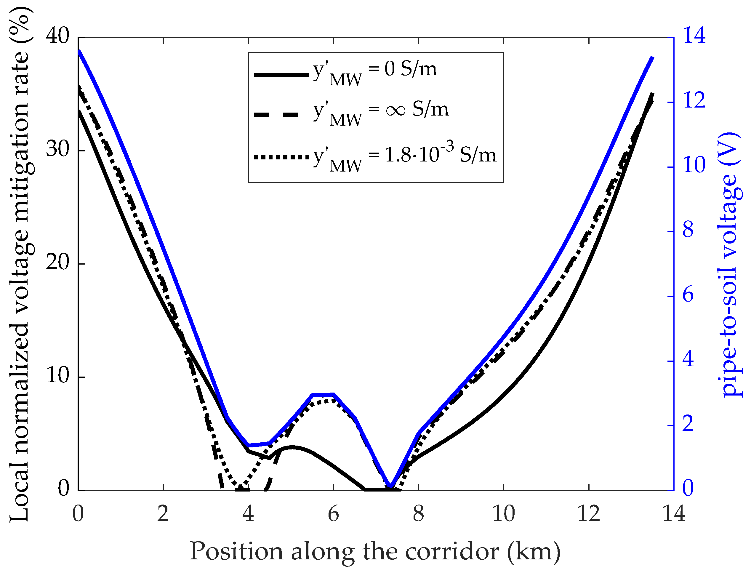
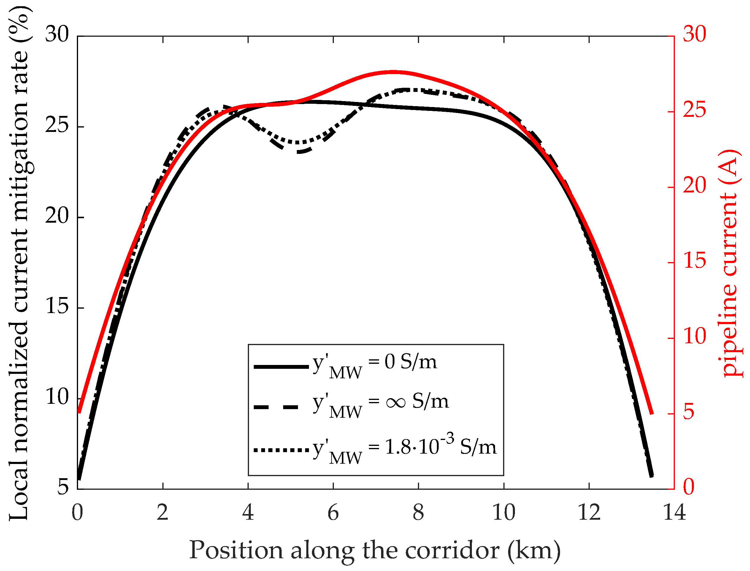
4.5. Local Mitigation Rate Assessment

Finally, Figure 9 and Figure 10 depict the local normalized voltage and current mitigation rates along the corridor when cylindrical mitigation wires are employed, respectively. The mitigation rate in Equation (4) is referred to the section of the corridor corresponding to the maximum unmitigated voltage or current, whereas the local mitigation rate is defined as:

$$M{R}_{V,local}=\left(1-\frac{V_{p-s}}{V_{pipe,0}}\right)·100.$$

(5)

Equation (5) expresses the local voltage mitigation rate; the definition of the local current mitigation rate is analogous:

$$M{R}_{I,local}=\left(1-\frac{I_{pipe}}{I_{pipe,0}}\right)·100.$$

(6)

A normalized local mitigation rate is defined as follows, for the induced voltage and current, respectively:

$$M{R}_{V,local,norm}=\frac{V_{p-s}}{max\left(V_{p-s}\right)}\left(1-\frac{V_{p-s}}{V_{p-s,0}}\right)·100.$$

(7)

$$M{R}_{I,local,norm}=\frac{I_{p-s}}{max\left(I_{p-s}\right)}\left(1-\frac{I_{pipe}}{I_{pipe,0}}\right)·100.$$

(8)

The unmitigated voltage-to-soil and current are shown in the right axis of Figure 9 and Figure 10, for reference.

5. Conclusions

The results show that screening conductors can be an effective and practical way to reduce the voltage and current induced in a buried metallic pipeline by induced coupling. The mitigation rates obtained with cylindrical and square cross-section wires are similar. This result can be explained by the fact that in both cases the skin depth is larger than the wire characteristic size, then making the current density distribution approximately uniform on the wire cross-section.

The obtained results highlight that the ratio between the mitigation rates yielded by the different admittances to earth is not constant over the whole corridor. Nevertheless, the marked variations of $M{R}_V$ that are visible in the middle part of the corridor in Figure 9 are not particularly significant, due to the low local value of induced voltage (depicted in blue). Conversely, significant variations of the obtained mitigation efficacy are visible in Figure 10 in the middle part of the corridor, when the mitigation wires are assumed to be perfectly insulated from the soil.

In both cases, also taking into account the results in Table 3 and Table 4, it can be noticed that different values for ${\underline{y}}_{MW-s}^{\prime }$ yield non negligible differences in the computed mitigation efficacies.

In particular, the assumption of ${\underline{y}}_{MW-s}^{\prime }=0$ leads to an underestimation of the mitigation rate, both for $M{R}_V$ and $M{R}_I$. Conversely, assuming that ${\underline{y}}_{MW-s}^{\prime }=\infty$ leads to results that are considerably closer to the practical value of ${\underline{y}}_{MW-s}^{\prime }=1.8\times {10}^{-3}\mathrm{S}/\mathrm{m}$. Nevertheless, if ${\underline{y}}_{MW-s}^{\prime }$ is of difficult estimation, the choice of ${\underline{y}}_{MW-s}^{\prime }=0$ represents a safe guess.

References

1. IEEE Guide for Evaluating AC Interference on Linear Facilities Co-Located Near Transmission Lines. IEEE Std. 2020, 1–49. [CrossRef]
2. Lucca, G. AC interference from a faulty power line on nearby buried pipelines: Influence of the surface layer soil. IET Sci. Meas. Technol. 2020, 14, 225–232. [Google Scholar] [CrossRef]
3. Ding, H.; Zhang, Y.; Gole, A.; Woodford, D.; Han, M.; Xiao, X. Analysis of coupling effects on overhead VSC-HVDC transmission lines from AC lines with shared right of way. IEEE Trans. Power Deliv. 2010, 25, 2976–2986. [Google Scholar] [CrossRef]
4. CIGRE. Guide on the Influence of High Voltage AC Power Systems on Metallic Pipelines; Technical Report; Cigré Working Group 36.02: Paris, France, 1995; pp. 1–135. [Google Scholar]
5. Dabkowski, J. How to predict and mitigate A. C. voltages on buried pipelines. Pipeline Gas J. 1979, 206, 19–21. [Google Scholar]
6. Adedeji, K.; Ponnle, A.; Abe, B.; Jimoh, A.; Abu-Mahfouz, A.; Hamam, Y. A review of the effect of ac/dc interference on corrosion and cathodic protection potentials of pipelines. Int. Rev. Electr. Eng. 2018, 13, 495–508. [Google Scholar] [CrossRef] [Green Version]
7. Mariscotti, A. Induced Voltage Calculation in Electric Traction Systems: Simplified Methods, Screening Factors, and Accuracy. IEEE Trans. Intell. Transp. Syst. 2011, 12, 201–210. [Google Scholar] [CrossRef]
8. Barthold, L.; Finney, W.; Lambert, E.; Skelton, H.; Schlomann, R.; Zaffanella, L.; Williams, P.; Clark, C.; Hubbard, D.; Delaplace, L. Electromagnetic effects of overhead transmission lines practical problems, safeguards, and methods of calculation. IEEE Trans. Power Appar. Syst. 1974, PAS-93, 892–904. [Google Scholar] [CrossRef]
9. Dushimimana, G.; Simiyu, P.; Ndayishimiye, V.; Niringiyimana, E.; Bikorimana, S. Induced electromagnetic field on underground metal pipelines running parallel to nearby high voltage AC power lines. E3S Web Conf. 2019, 107, 02004. [Google Scholar] [CrossRef]
10. Lucca, G. AC interference from faulty power cables on buried pipelines: A two-step approach. IET Sci. Meas. Technol. 2021, 15, 25–34. [Google Scholar] [CrossRef]
11. Tleis, N. Power Systems Modelling and Fault Analysis; Elsevier Ltd.: Amsterdam, The Netherlands, 2008. [Google Scholar]
12. Dawalibi, F.P.; Southey, R.D. Analysis of electrical interference from power lines to gas pipelines. I. Computation methods. IEEE Trans. Power Deliv. 1989, 4, 1840–1846. [Google Scholar] [CrossRef]
13. Chrysostomou, D.; Dimitriou, A.; Kokkinos, N.; Charalambous, C. Short-term electromagnetic interference on a buried gas pipeline caused by critical fault events of a wind park: A realistic case study. IEEE Trans. Ind. Appl. 2020, 56, 1162–1170. [Google Scholar] [CrossRef]
14. Kopsidas, K.; Cotton, I. Induced voltages on long aerial and buried pipelines due to transmission line transients. IEEE Trans. Power Deliv. 2008, 23, 1535–1543. [Google Scholar] [CrossRef]
15. Micu, D.D.; Christoforidis, G.C.; Czumbil, L. AC interference on pipelines due to double circuit power lines: A detailed study. Electr. Power Syst. Res. 2013, 103, 1–8. [Google Scholar] [CrossRef]
16. Christoforidis, G.C.; Labridis, D.P.; Dokopoulos, P.S. Inductive interference on pipelines buried in multilayer soil due to magnetic fields from nearby faulted power lines. IEEE Trans. Electromagn. Compat. 2005, 47, 254–262. [Google Scholar] [CrossRef]
17. Zhu, M.; Yuan, Y.; Yin, S.; Yu, G.; Guo, S.; Huang, Y.; Du, C. Corrosion behavior of pipeline steel with different microstructures under AC interference in acid soil simulation solution. J. Mater. Eng. Perform. 2019, 28, 1698–1706. [Google Scholar] [CrossRef]
18. Luo, Y.; Lin, N.; Zhou, S.; Li, S.; Wang, H. Effects of electromagnetic interference and crevice on corrosion of natural gas pipelines. IOP Conference Series: Earth and Environmental Science. IOP Publ. 2021, 675, 012061. [Google Scholar]
19. Chen, L.; Du, Y.; Liang, Y.; Li, J. Research on corrosion behaviour of X65 pipeline steel under dynamic AC interference. Corros. Eng. Sci. Technol. 2021, 56, 219–229. [Google Scholar] [CrossRef]
20. Gouda, O.; Dein, A.; El-Gabalawy, M. Effect of electromagnetic field of overhead transmission lines on the metallic gas pipe-lines. Electr. Power Syst. Res. 2013, 103, 129–136. [Google Scholar] [CrossRef]
21. CIGRE. AC Corrosion on Metallic Pipelines Due to Interference from AC Power Lines—Phenomenon, Modelling and Countermeasures; Technical Report; Cigré Working Group C4.2.02: Paris, France, 2006; pp. 1–110. [Google Scholar]
22. Chuco Paucar, B.; Roel Ortiz, J.L.; Pereira Pinto, J.O.; Koltermann, P.I. Induced voltage on gas pipeline with angle between a transmission line. In Proceedings of the 2007 IEEE Lausanne POWERTECH, Lausanne, Switzerland, 1–5 July 2007; pp. 796–800. [Google Scholar]
23. Popoli, A.; Sandrolini, L.; Cristofolini, A. Inductive coupling on metallic pipelines: Effects of a nonuniform soil resistivity along a pipeline-power line corridor. Electr. Power Syst. Res. 2020, 189, 106621. [Google Scholar] [CrossRef]
24. Popoli, A.; Sandrolini, L.; Cristofolini, A. Comparison of Screening Configurations for the Mitigation of Voltages and Currents Induced on Pipelines by HVAC Power Lines. Energies 2021, 14, 3855. [Google Scholar] [CrossRef]
25. Popoli, A.; Cristofolini, A.; Sandrolini, L. A numerical model for the calculation of electromagnetic interference from power lines on nonparallel underground pipelines. Math. Comput. Simul. 2021, 183, 221–233. [Google Scholar] [CrossRef]
26. Popoli, A.; Sandrolini, L.; Cristofolini, A. A quasi-3D approach for the assessment of induced AC interference on buried metallic pipelines. Int. J. Electr. Power Energy Syst. 2019, 106, 538–545. [Google Scholar] [CrossRef]
27. Steele, C.W. Numerical Computation of Electric and Magnetic Fields; Springer Science & Business Media: Berlin/Heidelberg, Germany, 2012. [Google Scholar]
28. Popoli, A.; Sandrolini, L.; Cristofolini, A. Finite Element Analysis of Mitigation Measures for AC Interference on Buried Pipelines. In Proceedings of the 2019 IEEE International Conference on Environment and Electrical Engineering and 2019 IEEE Industrial and Commercial Power Systems Europe (EEEIC/I&CPS Europe), Genova, Italy, 11–14 June 2019; pp. 1–5. [Google Scholar] [CrossRef]
29. Hayashi, T.; Mizuno, Y.; Naito, K. Study on Transmission-Line Arresters for Tower with High Footing Resistance. IEEE Trans. Power Deliv. 2008, 23, 2456–2460. [Google Scholar] [CrossRef]
30. Yadee, P.; Premrudeepreechacharn, S. Analysis of Tower Footing Resistance Effected Back Flashover Across Insulator in a Transmission System. In Proceedings of the International Conference on Power Systems, Lyon, France, 4–7 June 2007. [Google Scholar]
31. Theethayi, N.; Thottappillil, R.; Paolone, M.; Nucci, C.A.; Rachidi, F. External impedance and admittance of buried horizontal wires for transient studies using transmission line analysis. IEEE Trans. Dielectr. Electr. Insul. 2007, 14, 751–761. [Google Scholar] [CrossRef]
32. ITU-T. CCITT Directives Volume {III}: Calculating Induced Voltages and Currents in Pratical Cases; Technical Report; ITU-T: Geneva, Switzerland, 1989. [Google Scholar]
33. Cristofolini, A.; Popoli, A.; Sandrolini, L. Numerical Modelling of Interference from AC Power Lines on Buried Metallic Pipelines in Presence of Mitigation Wires. In Proceedings of the 2018 IEEE International Conference on Environment and Electrical Engineering and 2018 IEEE Industrial and Commercial Power Systems Europe (EEEIC/I&CPS Europe), Palermo, Italy, 12–15 June 2018; pp. 1–6. [Google Scholar] [CrossRef]
Figure 1. Pipeline horizontal position with respect to the HVAC power line along the length of the corridor (routing).
Electricity 02 00019 g001
Figure 2. Geometric characteristics of the considered power line, pipeline and mitigation wires.
Electricity 02 00019 g002
Figure 3. Magnitude of the induced pipe-to-soil voltage and longitudinal pipe current along the corridor, when no mitigations measures are put in place.
Electricity 02 00019 g003
Figure 4. Magnitude of induced pipe-to-soil voltage and longitudinal pipe current along the corridor, when 4 equispaced cylindrical mitigation wires are employed.
Electricity 02 00019 g004
Figure 5. Magnitude of induced pipe-to-soil voltage and longitudinal pipe current along the corridor, when 4 equispaced square mitigation wires are employed.
Electricity 02 00019 g005
Figure 6. Magnitude of induced pipe-to-soil voltage and longitudinal pipe current along the corridor, when a single conductive sheet is buried above the pipeline.
Electricity 02 00019 g006
Figure 7. Current density magnitude distribution in a square mitigation wire.
Electricity 02 00019 g007
Figure 8. Current density magnitude distribution yielded by the FEM analysis when a single conductive sheet is buried above the pipeline.
Electricity 02 00019 g008
Figure 9. Normalized local mitigation rate along the corridor for three different values of p.u.l admittance to earth of the four (cylindrical) mitigation wires (left axis); unmitigated pipe-to-soil voltage (right axis).
Electricity 02 00019 g009
Figure 10. Normalized local current mitigation rate along the corridor for three different values of p.u.l. admittance to earth of the four (cylindrical) mitigation wires (left axis); unmitigated pipeline current (right axis).
Electricity 02 00019 g010