Abstract
This paper presents a study and proposes a new methodology to analyze, evaluate and reduce the overall uncertainty of instrumentations for EMC measurements. For the scope of this work, the front end of a commercial EMI receiver is chosen and variations due to tolerances, temperature and frequency response of the system are evaluated. This paper illustrates in detail how to treat each block composing the model by analyzing each discrete component, and how to evaluate their influence on the measurand. Since a model can have hundreds or even thousands of parameters, the probability distribution functions (PDFs) of some variable might be unknown. So, a method that allows to obtain in a fast and easy way the uncertainty of the measurement despite having so many variables, to then being able to evaluate the influence of each component on the measurand, is necessary for a correct design. In this way, it will be possible to indicate which discrete components have the most influence on the measurand and thus set the maximum tolerances allowed and being able to design a cost-effective solution. Furthermore, this works presents a methodology which can easily be extended and applied to estimate and compute the uncertainty for electromagnetic interferences, energy storage systems (ESS), energy production, electric machines, electric transports and power plants in general.
1. Introduction
It is well known how different parameters can affect electrical components, affecting not only their nominal value, but also increasing their degradation over time and consequently reducing their estimated lifetime [1,2,3,4]. Furthermore, frequency has a strong impact on electrical components and parasitic components can give rise to problems that were not considered in the design phase [5,6,7,8,9,10,11].
The need to define the measurement uncertainty comes from the fact that every component which constitutes any kind of system shows a nominal value which is not fixed, but rather changes according to different probability distribution functions (PDFs) [11,12,13,14,15].
Having an accurate way to assess the uncertainty value of the measurand, especially if this value is the result of a combination of various parameters along the measurement chain is fundamental [16,17,18,19]. This information becomes fundamental when, for instance, the measurement is published in official product specifications or national standards.
To evaluate the uncertainty propagation The Guide to expression of Uncertainty in Measurement (GUM) is nowadays considered the reference standard.
The GUM offers different approaches to obtain the PDF of the final measurand. The last introduced approach is the Monte Carlo Method (MCM), based on the concept of associating a PDF to each input variable to obtain the PDF of the final measurand [11,12,13,14].
It is important to underline that these methods are based on a linear approximation of the model, so MCM results will be approximate and never exact, but still they are considered a reference model to evaluate uncertainty propagation [11,12,13,14,15].
The measurement uncertainty evaluated for electromagnetic compatibility (EMC) is a critical factor because a product can comply or not with the applicable standards depending on the result and associated uncertainty obtained [20].
Especially in EMC testing, different conditions, test sites and external factors can have an impact on the measurement uncertainty and reproducibility. For instance, the uncertainty of conducted emissions measurements can be affected by the lengths of the cables [21], the position of the device under test (DUT), straight capacitances and height, while radiated emissions could be influenced by several set-up conditions like the material of the table where the DUT is posed, rotating table position, etc. [22,23].
The standards which regulate conducted and radiated emissions measurement uncertainty, CISPR 32:2015 [24] CISPR 16-4-2 [25], do not specifically define how RF cables shall be placed and the table material, therefore the uncertainty associated with the measurement is higher than expected.
Consequently, these days EMC measurement uncertainties have not been studied enough and there is the need of further study and research to have a homogeneous characterization. This is the major reason of why mixed and combined uncertainties are still not known and why a more in deep knowledge of uncertainty in EMC measurements must be reached [11].
In this paper, a new methodology to evaluate the measurement uncertainty and determine which discrete component, or groups of components, have the most influence on the measurand is proposed. This method consists of different steps: first the uncertainty of the measurand is evaluated by means of Monte Carlo simulations and then, the influence of each parameter due to tolerance variations and other external factors on the final measurand is calculated. Then a methodology to evaluate and choose the optimum parameters to limit the influence on the measurand uncertainty is presented. This method is finally applied on a commercial EMC receiver as a test case.
The approach proposed in this paper can also be applicable, in a general way, to other instruments, parameters, models and external factors that influence the measurand uncertainty. Different applications can also be faced by using the methodology proposed. For instance, calculating the uncertainty for renewable energy sources (RES), provide an estimation of uncertainty of power flowing in overhead and underground power line and electromagnetic pollution and its associated uncertainty is feasible with the approach presented in this paper.
The paper is organized as follows: Section 2 provides an overview of the existing studies and works on how to evaluate the influence on the measurand of external factors and method commonly used [1,2,3,4,6,7,8,9,10,11]. Section 3 is dedicated at describing the proposed methodology and the instrument used for its verification. In Section 4 the results arising from a real case scenario are presented and discussed to verify the effectiveness and the advantages proposed by the presented method. Finally, Section 5 summarizes a final discussion on the work.
2. Factors of Influence Evaluation
It is necessary to understand how the metrological behavior of an instrument is affected by all the external factors that it can be subjected to. Any electrical component is affected by changes in temperature, humidity, geometry and the applied electrical field [1,2,3,4]. Depending on the operating conditions and the design chosen, each of the aforementioned quantities can have a stronger impact than others [8,9]. Since the instrument analyzed in this paper is an EMI receiver for measurements of conducted emission, its operating condition is not affected by geometry or environmental conditions since once designed its geometry cannot change and it is intended for use in environments, for example laboratories, where humidity is under control. Focus is therefore posed on the temperature variation which can arise due to overheating of FPGAs, amplifiers or any other active components, the tolerances and the frequency response of the model.
2.1. Temperature Effect on Electrical Components
Each electrical component is subject to variation of its nominal values and performances when temperature changes. For instance, every manufacturer must publish in their datasheet information about ppm/°C and the temperature coefficient resistance (TCR). The TCR, measured in ppm/°C, shows the relative change of resistance per degree of temperature change:
where R1 is the resistance at room temperature, R2 is the resistance at the operating temperature, T1 is the room temperature while T2 is the operating temperature. The reference, or room temperature, is usually set at +25 °C [9].
Every manufacturer sets their own method to evaluate and define the TCR. Most of the times the lack of information about how this was done does not allow end users to calculate and predict the measurement uncertainty due to temperature changes. This issue becomes more important when high precision resistors and final uncertainty propagation are fundamental parameters.
2.2. Thermal Aging
It is well known how temperature has an effect not only on the parameter’s values but also on the lifespan itself [1,2,3,4]. Several examples are proposed in [1], where a complete analysis of exponential and inverse power model is presented [1,2].
Regarding thermal aging, the model widely accepted is the Arrhenius one:
where: K is Boltzmann constant, L′ is the life for θ = ∞, θ the absolute temperature and Ae the activation energy of the degradation process. When θ0 is assume as a reference, a number that can be chosen within the specification provided by the manufacturer, and the thermal aging is neglected for T = θ0 then the following expression holds:
Then it is possible to obtain:
where L0 is the estimated life at θ0.
When Equation (4) is plotted in a log graph Lt vs. T, it gives a straight line, where − indicates its slope. Equation (4) is also found in the IEC Standard 216 [10].
2.3. Variations Due to Parasitic Components
Due to manufacturing procedures and imperfections, the frequency response of inductors, capacitors and resistors is never ideal [5,6]. To take into consideration this effect, the equivalent series inductance (ESL) and the equivalent series resistance (ESR) have been introduced. ESR is used to calculate actual losses in capacitors and inductors, which are proportional to the R value while the ESL is important to consider the combination of Ls and Cs of various resonant circuits [4,5]. It has been practically demonstrated that capacitors ranging from 0.5 pF to 330 pF the ESL do not usually exceed 1 nH [4]. Another important parameter to consider is the Q factor. This parameter represents the energy dissipated in thermal losses inside the capacitor.
The Q factor must be considered in the design phase since it can affect how temperature dissipates around the instrument. Nowadays integrated circuits tend to be smaller and smaller, so the dimensions of and space between different components is extremely reduced. This must be considered during engineering simulations or when practically measuring the temperature that can be reached inside an equipment because it has severe impact on how to design the dissipation system [7].
where f is the frequency, C the nominal value of capacitor and R the equivalent series resistance.
2.4. The GUM Supplement 1
The GUM defines measurement uncertainty as a “parameter, associated with the result of a measurement, that characterizes the dispersion of the values that could reasonably be attributed to the measurand”. Basically, it defines how the standard uncertainty u(y) is associated with the result y of a measurement for the quantity Y as the parameter above mentioned. depends on different input quantities x1 … xn [11]:
With its associated standard uncertainty as:
where xi and xj are the estimate of Xi and Xj.
According to the GUM, the calculation of the measurand uncertainty has to be based on the law of the propagation of the error and the central limit theorem [14]. The GUM Supplement 1 states that in cases where it is difficult to assess whether or not the GUM framework is valid, Monte Carlo simulations provide a wide-accepted method to evaluate uncertainty propagation [12,13,14]. In practice, different PDFs can be assigned to the input variables of a model. The most common ones, and the ones that will be used in the simulations, are described here:
- ▪
- Rectangular Distribution:
This PDF reflects the principle of the maximum entropy, typically it is applied to parameters that present at least one of the following characteristics:
- ○
- There is no way to establish which value the parameter will assume within the proposed interval [a; b].
- ○
- All the values inside the aforementioned interval have the same probability.
- ○
- The parameter can assume a non-null value only in this finite interval, and is 0 elsewhere:
Its mean value is defined as follows:
While its variance, defined as the square of the standard deviation is:
The standard deviation can be obtained evaluating the standard uncertainty associated with the estimation of .
The rectangular PDF represented in Figure 1 is assigned to parameters that are known to vary within a fixed interval, but no information on the probability to have a certain value is known. Usually, manufacturers of components assign this PDF to their components in their datasheet, stating that the actual value of the parameter will vary from its nominal value in a specified interval, but no additional information is provided on the probability to assume a certain value [15,16].
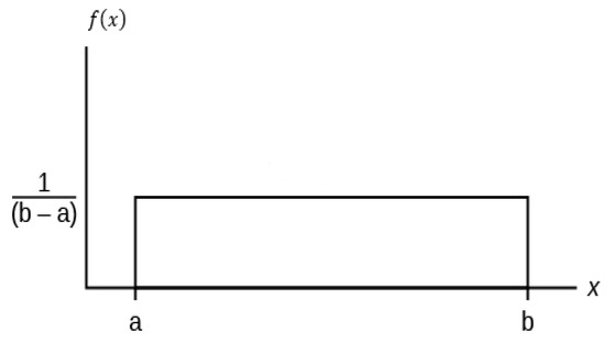
Figure 1.
Probability density function of a rectangular distribution.
- ▪
- Triangular Distribution
This PDF is used with parameters that present the following features:
- ○
- They have a finite value different from 0 in a finite interval [b; a].
- ○
- They have the highest probability to assume a value c, which is part of the interval [b; a].
- ○
- The probability from b to c and c to a change linearly.
- ○
- The relationship between different variables is known, but collecting more data is too complicated.
The term f(x) assumes the following values:
- ○
- 0 for x < a and b < x
- ○
- for c = x.
The mean value of f(x) is:
While its variance, defined as the square of the standard deviation is:
This distribution, represented in Figure 2, is based on a guess of the modal value of the parameter and it is usually used when data are limited and the relationship between different variables is known but collecting more data is too complicated. It is also called “lack of knowledge “distribution.
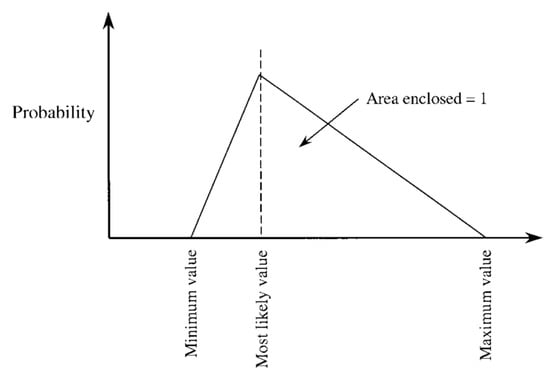
Figure 2.
Probability density function of a triangular distribution.
- ▪
- Gaussian Distribution
This PDF is applied to a quantity who is continuously fluctuating. This is the commonly used distribution to model statistic properties of physical quantities and its distribution is shown in Figure 3.
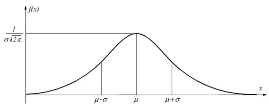
Figure 3.
Probability density function of a Gaussian, or normal, distribution.
f(x) is unimodal, symmetric, and characterized by:
- µ: mean value;
- σ: standard deviation.
Independently from the number n of input variables, the uncertainty propagation with MCMs simulation can be generally carried out considering Equation (6). The number of input variables represented in Figure 4 serves only an illustrative purpose [11,12].
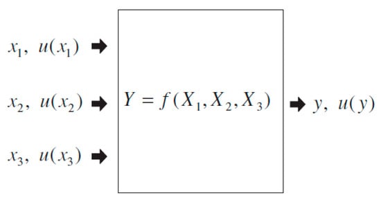
Figure 4.
Propagation of uncertainties for 3 input quantities.
According to the GUM, the uncertainty propagation can be calculated using Equations (6) and (7) where x1, x2 and x3 are the input quantities and u(x1), u(x2) and u(x3) are the respective uncertainties and y and u(y) are the measurand with its uncertainty.
Any PDF can be assigned to the input quantities, depending on various assumption that have been explained in the previous section. For instance, in Figure 5 the input quantities , and are described by their PDF, in this case are Gaussian, triangular and again Gaussian, still Figure 4 and Figure 5 are used as a representative example.

Figure 5.
Illustration of the propagation of distributions for N = 3 independent input quantities.
3. Proposed Methodology
When designing the measurement chain of an instrument and evaluating its uncertainty propagation and trying to reduce it, the components that have the most impact on the overall uncertainty must be identified. The methodology presented in the following sections proposes a simple way to analyze each discrete component of the model of the DUT and allows to determine the ones which have more influence on the measurand. By identifying the components which bring more contribution to the overall uncertainty, whether it is due to tolerances variations or influences of external factors, it is possible to set the maximum tolerances allowed and technical performances required.
To this end, different PDFs will be assigned to input variables the evaluate how the overall uncertainty of the measurand for real case scenarios. Rectangular PDFs are typically the most used ones because they reflect the principle of maximum entropy and assume the worst-case scenario, but not all parameters are subjected to the same temperature gradient and their distribution also depends on manufacturing process, geometry, and ventilation [15,16]. This is the reason why an approach that considers different PDFs will be used.
3.1. Analysis of the Measurand Uncertainty
To make sure that the uncertainty is kept within a determined range it is fundamental to know which parameters have the most influence on the final measurand. According to [18,19] it is possible to evaluate the parameter influence in different ways. In this paper the following approach has been used:
where PI is the parameter influence, Vexpected is the expected mean value, Vout_res is the value obtained when the model is computed and only 1 parameter is changed at a time and h = max(Vout_res − Vexpected) is the maximum value obtained by evaluating the model when one parameter changes, according to its PDF, at a time. Equation (15) is iterated for all the components of the model.
3.2. Process Steps
The whole process is summarized here:
- (1)
- The overall measurement uncertainty is determined by performing Monte Carlo simulations (MCMs).
According to the datasheet and manufacturer information, different PDFs are assigned to each parameter composing the measurement chain. Not all parameters have the same PDFs, nor they are subjected to the same temperature gradients. Furthermore, each component presents a different behavior, so a combination of rectangular and triangular PDFs has been chosen to provide a full overview of the results that can be obtained whether using data provided by manufacturers or by assuming another type of PDF to overcome the lack of information. A triangular distribution has been assigned to components, especially the ones distant from ADCs or amplifiers, which are not subject to a wide range of temperature variation, and it is safe to assume that their deviation from nominal value is lower than others.
- (2)
- A sensitivity analysis is performed. Equation (15) is evaluated, and PI is determined for each component of the model.
Other studies on uncertainty evaluations which can be found in literature, like the ones proposed in [6,11,12,13,14], do not include a sensitivity analysis, so no information on which parameters affect the overall uncertainty is provided. This is useful only if the objective is to evaluate, but not to minimize, the uncertainty.
- (3)
- The parameters of the model of Figure 6 are grouped depending on their influence. For instance, the following classification has been used:
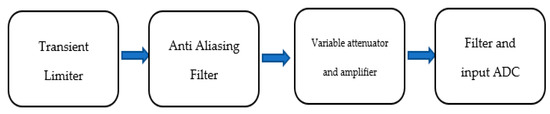 Figure 6. Block diagram of the input part of the considered receiver.Group A: Includes parameters that strongly affect the measurand, PI > 0.4.Group B: Includes parameters that slightly affect the measurand, 0.1 < PI < 0.4.Group C: Includes parameters that do not affect the measurand, PI < 0.1.
 - (4)
- MCMs simulations can be performed again. The number N remains unchanged. This time, to consider the worst-case scenario, only rectangular PDFs are considered. The result obtained is compared with the previous one obtained in Step 1 and the difference must be acceptable by manufacturer. This step is recommended to increase the reliability of the proposed methodology, but it is not mandatory if small variation from results obtained in Point 1 are not critical for the instrument.
- (5)
- A second sensitivity analysis to consider variation due to temperature gradient is performed. Components which have the most influence on the measurand are now identified. The following classification has been used:Group A′: Includes parameters that strongly affect the output measurand, PI > 0.4.Group B′: Includes parameters that slightly affect the output measurand, 0.1 < PI < 0.4.Group C′: Includes parameters that do not affect the output measurand, PI < 0.1.
- (6)
- The two set of groups are analyzed in the following way:
- -
- If a parameter belongs to group A and A′, it is fundamental to choose one to have the best performances and the most reliable.
- -
- If a parameter belongs to group A-B′ then it is fundamental that its tolerance is as low as possible, but it is less important its exposure to temperature variation.
- -
- On the contrary, if a parameter is identified to be in group C-A′, it is not important its tolerance, but it is important that the temperature variation is controlled and kept as low as possible.
For sake of simplicity, the presented methodology is hereafter represented in a flowchart shown in Figure 7.
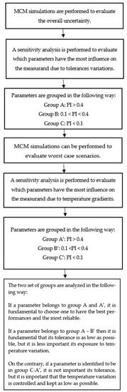
Figure 7.
Flowchart of the presented methodology.
3.3. Description of the Analog Front End of the Receiver Used to Evaluate the Proposed Method
The method proposed in the previous section has been applied to evaluate the input stage of the EMSCOPE, a commercial double channel EMI receiver for measurements of conducted emissions up to 110 MHz, manufactured by EMZER Technological Solutions SL (Barcelona, Spain). The block diagram is shown in Figure 6, while the instrument is shown in Figure 8.
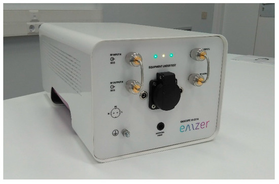
Figure 8.
Picture of the commercial EMI Receiver for conducted emissions analysed.
Each of the blocks is composed of variables and parameters that propose a fully internal characterization of the instrument. In detail:
- -
- Transient limiter: the transient protects the sensitive input of the receiver from unwanted signals coming though the line impedance stabilization network (LISN). This block is composed by a high pass filter (HPF) and a pulse limiter with 10 dB attenuation.
- -
- Anti-aliasing filter: Includes filtering components, basically capacitors and inductors, which filters frequency which are not in the wanted frequency range.
- -
- Variable attenuators and amplifiers: the input signal is changed to an amplitude level to be correctly measured.
- -
- Filter and input ADC: part where analog to digital conversion and additional filtering is performed.
The blocks represented in Figure 6 are in cascade. There is no direct interaction among them. Basically, the uncertainty coming from one is the direct input of the following one. Every variation, uncertainty contribution and unwanted anomaly introduced in each of these blocks will increase overall uncertainty of the instrument. Table 1 summarizes the symbols and characteristics of each discrete component composing the blocks of the analyzed Figure 6.

Table 1.
Description of the components of the model.
To model in Simulink environment the blocks represented in Figure 6, the following procedure has been used:
- (A)
- Each discrete component has been created and modeled in a Simulink environment.
- (B)
- The final output, the measurand, has been chosen.
- (C)
- The variables that affect the measurand have been defined and their effects modeled.
- (D)
- Different PDFs have been assigned to each variable according to the data furnished by the manufacturers and the principle explained in the previous sections.
- (E)
- The uncertainties have been propagated thought the model and the final PDF of the measurand has been obtained and evaluated.
- (F)
- Step E has been replicated throughout the whole frequency range.
4. Results
The methodology proposed in Section 3.2 has been applied to the EMI receiver described in Section 3.3.
The results have been obtained considering the following scenario:
The expected mean value of the block chain attenuation is obtained by fixing the gain of the variable attenuators and amplifiers shown in Figure 6 to 0 dB, so that the whole chain offers an expected attenuation of 10 dB. A temperature variation of ± 20 °C from the standard reference temperature of ±25 °C has been considered.
Table 2 shows the results obtained when MCMs simulations are performed. The number N of iteration has been set at 6.000 and a combination of PDFs has been assigned to the input variables according to Point 1 and 4 described in Section 3.2.
Table 2.
Results obtained with combination of PDFs according to Point 1 and 4 of Section 3.2.
As it can be seen in Figure 9, the measurand has a normal distribution, with the mean value centered in 10 dB and the standard deviation ranging from 0.09 to 0.13, depending on the PDFs assigned.
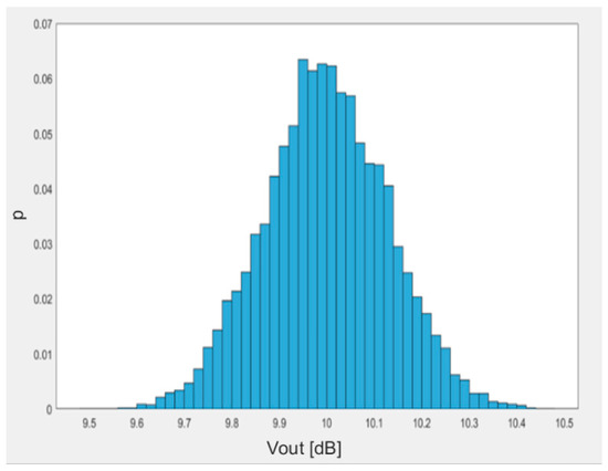
Figure 9.
Distribution of the output voltage obtained with mixed PDFs.
Figure 10 shows the frequency response of the attenuator block and its variation from nominal value when mixed PDFs are implemented to consider the tolerances of the components, the temperature is now kept at reference value so only the uncertainty coming from components tolerances is evaluated. As it can be seen, the mean value is maintained throughout the whole frequency span and the maximum variation is kept within 10 dB ± 0.3.
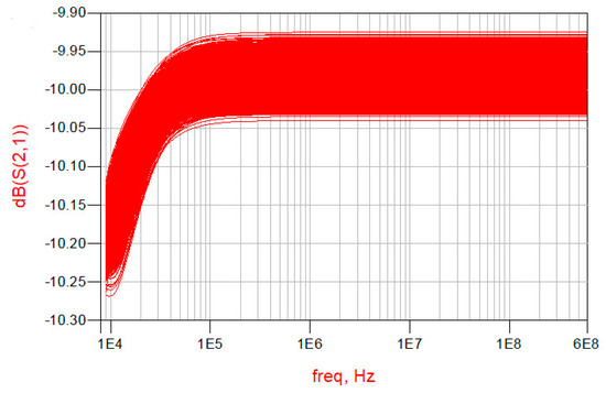
Figure 10.
Frequency vs. Vout [dB].
4.1. Evaluation of the Parameter Influence on the Measurand and Proposed Design Techniques
The scope of this paper is to propose a methodology for to evaluate how variations due to temperatures and tolerances affect the overall uncertainty and frequency response of the system and how to reduce it. To this end, steps 3 and 5 of Section 3.2 have been computed. The components of the model shown in Figure 6 are named using a letter R, which stands for resistor, C for capacitor and L for inductor and a number. Figure 11 shows the results obtained when the influence of the parameters on the measurand is computed according to Equation (15). In this case, the tolerances have been considered as influence factors.
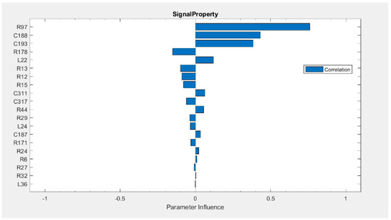
Figure 11.
Parameters influence on the measurand.
Considering the block chain described in Figure 6 and the results shown in Figure 11, the following components have been found to be in the level of influence A, B and in the level of influence C. In concrete the following groups are identified:
- Group A: R97, C188, C193.
- Group B: R178, L22, R13, R12, R15, C311,C317, R44.
- Group C: R29,L24,C187, R171, R24, R6, R27, R32, L36.
4.2. System Design According to the Proposed Methodology
The overall uncertainty of a system is minimized when the correct components are chosen. Extreme care should be taken because the choices made in this stage will have an impact on the overall uncertainty of the instrument.
If a decision is based only in the first set of simulations, according to Figure 11, the parameters belonging to group A will be the chosen in the most accurate way and, most likely, they will be more expensive. This choice would give good results in case external factors were not present at all, which is extremely unlikely in real case scenarios.
According to Point 6 of Section 3.2, another series of sensitivity analysis has been carried out to evaluate the effect of external factors. In this case a temperature variation of ±20 °C from the standard reference temperature of ±25 °C has been computed to evaluate the effect of temperature gradients on the measurand.
Thanks to the new methodology proposed in this paper, new results are obtained and shown in Figure 12, new groups are identified according to step 7, and are compared with the ones identified according to step 3. According to Point 6 of Section 3.2, another series of sensitivity analysis has been carried out to evaluate the effect of external factors. In this case a temperature variation of ±20 °C from the standard reference temperature of ±25 °C has been computed to evaluate the effect of temperature gradients on the measurand.
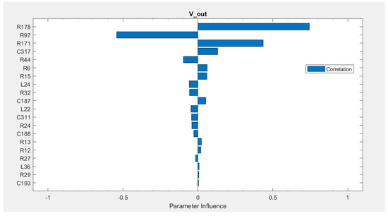
Figure 12.
Parameters influence on the measurand.
According to the results shown in Figure 12, the following components have been found to be in the level of influence A′, B′ and in the level of influence C′. In concrete the following groups are identified:
- Group A′: R178, R97, R171,
- Group B′: C317, R44, R6, R15, L24 R32, C187, L22,
- Group C′: C311, R24,C188, R13, R12, R27, L36, R29, C193.
In this particular case, it is possible to notice that parameter R171 belongs to group C and A′. This means that the temperature has a strong impact on this component and must be monitored closely.
The precautions that shall be taken are:
- (1)
- Choosing resistance with a low temperature coefficient.
- (2)
- Make sure the ventilation system, if available, or the heat sink are properly designed so that the temperature is kept as constant as possible.
Thanks to the results obtained, the manufacturer of the instrument has the necessary information to determine which components contribute more to the overall uncertainty. By simply acting only on these components, the uncertainty associated with the measurement can be reduced.
The authors would like to highlight that the methodology proposed is applied to a particular case scenario, but it remains a general method which can be applied in different fields and situations, it does not lose sense of generality. For instance, engineers who are involved in the design of a new instrument could use the methodology proposed to:
- (a)
- Evaluate the overall uncertainty propagation.
- (b)
- Identify which discrete components bring more contribution to the overall uncertainty and being able to reduce it.
5. Conclusions
This paper presents and validates, both from a mathematical and experimental point of view, a simple and new methodology which allows one to understand how to evaluate and properly chose components of the front end of an EMI receiver depending on their influence on the measurand.
This approach offers a simplified analysis to improve the overall uncertainty of any instrument for EMC testing or system, which may also include but not limited to estimating the uncertainty for electromagnetic pollution, electric vehicle (EV) charging stations, electric machines, energy storage systems (ESS), and power plants in general starting from the very first decision of which components to implement, a task often underestimated in the design phase.
The presented paper introduces a new methodology to evaluate the overall uncertainty of an EMI receiver for conducted emission measurements in an easier way than the one proposed in the standards, which can be used both in the design phase or later on, to ensure a stable overall uncertainty and a correct design technique is achieved.
Engineers dealing with choices which include, but are not limited to, selecting correct tolerance values of components while considering its PDFs, cost analysis depending on choosing components instead of others and their effect on the final accuracy of the whole instrument, appears to be the beneficiary of the methodology presented in the paper for their research works.
Author Contributions
Conceptualization, M.B.; supervision, L.P.; visualization, L.P.; writing—original draft, M.B.; writing—review & editing, A.-M.S. and F.J.P. All authors have read and agreed to the published version of the manuscript.
Funding
This research received no external funding.
Institutional Review Board Statement
Not applicable.
Informed Consent Statement
Not applicable.
Data Availability Statement
The data presented in the study are available in the article.
Conflicts of Interest
The authors declare no conflict of interest.
References
- Montanari, G.; Simoni, L. Aging Phenomenology and Modeling. IEEE Trans. Electr. Insul. 1993, 28, 755–776. [Google Scholar] [CrossRef]
- Douzi, S.; Tlig, M.; Slama, J.B.H. Experimental investigation on the evolution of a conducted-EMI buck converter after thermal aging tests of the MOSFET. Microelectron. Reliab. 2015, 55, 1391–1394. [Google Scholar] [CrossRef]
- Pennettaa, C.; Reggianib, L.; Kissc, L.B. Thermal effects on the electrical degradation of thin film resistors. Phys. A 1999, 266, 214–217. [Google Scholar] [CrossRef]
- Gurov, E.V.; Uvaysov, S.U.; Uvaysova, A.S. Analysis of the parasitic parameters influence on the analog filters frequency response. In Proceedings of the 2019 International Seminar on Electron Devices Design and Production (SED), Prague, Czech Republic, 23–24 April 2019. [Google Scholar]
- Campos, A.C.; Cardoso, K.R.; Cruz, V.P.; Fortes, M.Z. Frequency response of capacitive voltage dividers for evaluation of harmonic components. In Proceedings of the 2019 IEEE PES Innovative Smart Grid Technologies Conference—Latin America, Gramado, Brazil, 15–18 September 2019. [Google Scholar] [CrossRef]
- Mingotti, A.; Costa, F.; Pasini, G.; Peretto, L.; Tinarelli, R. Modeling capacitive low-power voltage transformer behavior over temperature and frequency. Sensors 2021, 21, 1719. [Google Scholar] [CrossRef] [PubMed]
- Yang, L.; Odendaal, W.G.H. Measurement-based method to characterize parasitic parameters of the integrated power electronics modules. IEEE Trans. Power Electron. 2007, 22, 54–62. [Google Scholar] [CrossRef]
- Morgan, V.T. Effects of frequency temperature, compression, and air pressure on the dielectric properties of a multilayer stack of dry kraft paper. IEEE Trans. Dielectr. Electr. Insul. 1998, 5, 125–131. [Google Scholar] [CrossRef]
- Azzumar, M.; Khairiyati, L.; Faisal, A. Determination of the standard resistor temperature coefficients and their uncertainties. J. Stand. 2019, 21, 219–228. [Google Scholar] [CrossRef]
- International Electrotechnical Commission. Guide for the determination of thermal endurance properties of electrical insulating materials. In IEC 216-1 Part 1: General Guidelines for Aging Procedures and Evaluation of Test Results; International Electrotechnical Commission: London, UK, 1990. [Google Scholar]
- Kovačević, A.; Brkić, D.; Osmokrović, P. Evaluation of measurement uncertainty using mixed distribution for conducted emission measurements. Measurement 2011, 44, 692–701. [Google Scholar] [CrossRef]
- Cox, M.G.; Siebert, B.R.L. The use of a Monte Carlo method for evaluating uncertainty and expanded uncertainty. Metrologia 2006, 43, 178–188. [Google Scholar] [CrossRef]
- International Organization for Standardization. Guide to the Expression of Uncertainty in Measurement; International Organization for Standardization: Geneva, Switzerland, 1993. [Google Scholar]
- JCGM. Evaluation of Measurement Data—Supplement 1 to the ‘Guide to the Expression of Uncertainty in Measurement’—Propagation of Distributions Using a Monte Carlo Method; International Organisation for Standardisation: Geneva, Switzerland, 2008. [Google Scholar]
- Azpúrua, M.; Tremola, C.; Paéz, E. Comparison of the GUM and MonteCarlo methods for the uncertainty estimation in electromagnetic compatibility testing. Prog. Electromagn. Res. B 2011, 34, 125–144. [Google Scholar] [CrossRef]
- Wubbeler, G.; Krystek, M.; Elster, C. Evaluation of measurement uncertainty and its numerical calculation by a Monte Carlo method. Meas. Sci. Technol. 2008, 19, 084009. [Google Scholar] [CrossRef]
- Mingotti, A.; Peretto, L.; Tinarelli, R.; Yiğit, K. Simplified approach to evaluate the combined uncertainty in measurement instruments for power systems. IEEE Trans. Instrum. Meas. 2017, 66, 2258–2265. [Google Scholar] [CrossRef]
- Gu, J.; Zhang, S.; Wang, B. Monte Carlo analysis for significant parameters ranking in RLV flight evaluation. Procedia Eng. 2015, 99, 1082–1088. [Google Scholar] [CrossRef][Green Version]
- Pendrill, L.R. Using measurement uncertainty in decision making and conformity assessment. Metrologia 2014, 51, S206. [Google Scholar] [CrossRef]
- Mariscotti, A. Measurement procedures and uncertainty evaluation for electromagnetic radiated emissions from large-power electrical machinery. IEEE Trans. Instrum. Meas. 2007, 56, 2452–2463. [Google Scholar] [CrossRef]
- Cacciato, M.; Cavallaro, C.; Scarcella, G.; Testa, A. Effects of connection cable length on conducted EMI in electric drives. In Proceedings of the IEEE International Electric Machines and Drives Conference (IEMD’99), Seattle, WA, USA, 9–12 May 1999; pp. 428–430. [Google Scholar]
- Beeckman, P.A. The influence of positioning tables on the results of radiated EMC measurements. In Proceedings of the International Symposium on Electromagnetic Compatibility (EMC 2001), Montreal, QC, Canada, 13–17 August 2001; Volume 1, pp. 475–480. [Google Scholar]
- Zombolas, C. The effects of table material on radiated field strength measurement reproducibility at open area test sites. In Proceedings of the International Symposium on Electromagnetic Compatibility (EMC 2001), Montreal, QC, Canada, 13–17 August 2001; Volume 1, pp. 260–264. [Google Scholar]
- International Electrotechnical Commission. CISPR 32:2015, Electromagnetic Compatibility of Multimedia Equipment—Emission Requirements; International Electrotechnical Commission: London, UK, 2015. [Google Scholar]
- International Electrotechnical Commission. CISPR 16-4-2 Ed.2: Specification for Radio Disturbance and Immunity Measuring Apparatus and Methods, Part 4-2: Uncertainties, Statistics and Limit Modelling–Measurement Instrumentation Uncertainty; International Electrotechnical Commission: London, UK, 2018. [Google Scholar]
Publisher’s Note: MDPI stays neutral with regard to jurisdictional claims in published maps and institutional affiliations. |
© 2021 by the authors. Licensee MDPI, Basel, Switzerland. This article is an open access article distributed under the terms and conditions of the Creative Commons Attribution (CC BY) license (https://creativecommons.org/licenses/by/4.0/).