1. Introduction
Microgrids are currently an extensive topic of discussion since such a concept presents a viable solution to allow the integration of distributed energy resources near loads without disturbing or contributing to the stability of the main grid. Those microgrids can operate either when connected to the main grid or disconnected (island mode). During island mode operation, the inertia provided from the main grid is no longer available, and the local grid becomes very sensitive to power changes (weak grid). To guarantee the adequate operation of the connected power converters, one of the key aspects is to ensure synchronization under the mentioned conditions.
The power converters control loop is normally fully or partially performed as in the synchronous reference frame (SRF), where voltage estimation becomes even more critical as the phase estimation errors are propagated to the synchronous voltage and current measurements through the Park transform. Additionally, methods such as droop control or the virtual synchronous generator demand stable frequency measurement/estimation to achieve robust and proper power-sharing. The phase-locked loop (PLL) is designed primarily to estimate the phase of the voltage fundamental frequency positive sequence, but it also allows to obtain a stable voltage amplitude and frequency as discussed in this paper. The importance of the phase angle estimation is addressed in [
1], where it is studied the dynamic impact of phase jumps in synchronous generators and power converters, which may be caused by the estimation error during the connection with the grid.
There are currently several techniques to achieve grid synchronization, though it is not possible to point to a single synchronization algorithm that can simultaneously be the most accurate, fastest, most robust and lightest for every grid condition. Therefore, it is naturally necessary to establish a compromise between different goal objectives or grid conditions before choosing a particular synchronization algorithm.
In accordance with [
2], there are two main methods to achieve grid synchronization: open-loop or closed-loop. In an open-loop approach, the phase angle is directly estimated from a filtered signal. In the closed-loop, there may exist a filtering stage but angle estimation is obtained through a closed-loop structure.
An open-loop and simple technique for grid synchronization is zero cross-detection, which allows synchronizing with the grid at every instant that the grid voltage crosses a reference zero. The synchronization is achieved through the detection of the zero-cross events and the generation of a rectangular waveform, accordingly. The resulting waveform allows to estimate the phase and frequency but only during the zero-cross instants; for that reason, it presents phase tracking slow dynamics and it is susceptible to external interference, leading to phase tracking errors [
3,
4]. With such a technique, synchronization is achieved for a single-phase system, twice per cycle. Additionally, voltage harmonics or measurement noise may lead to undesired zero-crossing detection if no filters are added. Another open-loop approach is the use of filters in the
frame and prior angle calculation through a trigonometric relationship. Some of those filters include the Butterworth low-pass filter, space vector filter, adaptive notch filter,
etc. As an alternative to digital filters, there can be found methods that suggest the use of discrete Fourier transform, Kalman filters, least mean square [
5], or sliding mode control [
6].
Another method, and the most common synchronization technique in grid-tied power converters, is the closed-loop approach known as the synchronous reference frame phase-locked loop (SRF-PLL). The SRF-PLL presents fast dynamics with a very low steady-state error when no low order harmonics exist and balanced conditions are considered [
7]. Such assumptions are unrealistic in most real cases, especially when considering weak grids. Hence, most of the advanced PLL algorithms consist of the application of techniques to extract the fundamental frequency positive sequence (FFPS) of the grid voltage and further phase tracking through the SRF-PLL [
8,
9,
10].
To extract the FFPS, the authors in [
11] suggest the application of a double synchronous reference frame: one rotating with the positive frequency and another in the opposite direction (negative sequence). A decoupling network is presented that allows the extraction of the positive sequence from the double SRF. Furthermore, a second-order low pass filter is applied at the output to reduce harmonics interference in the positive sequence synchronous voltage estimation.
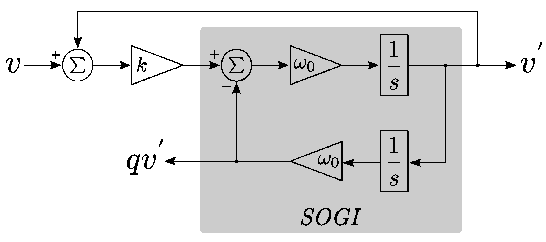
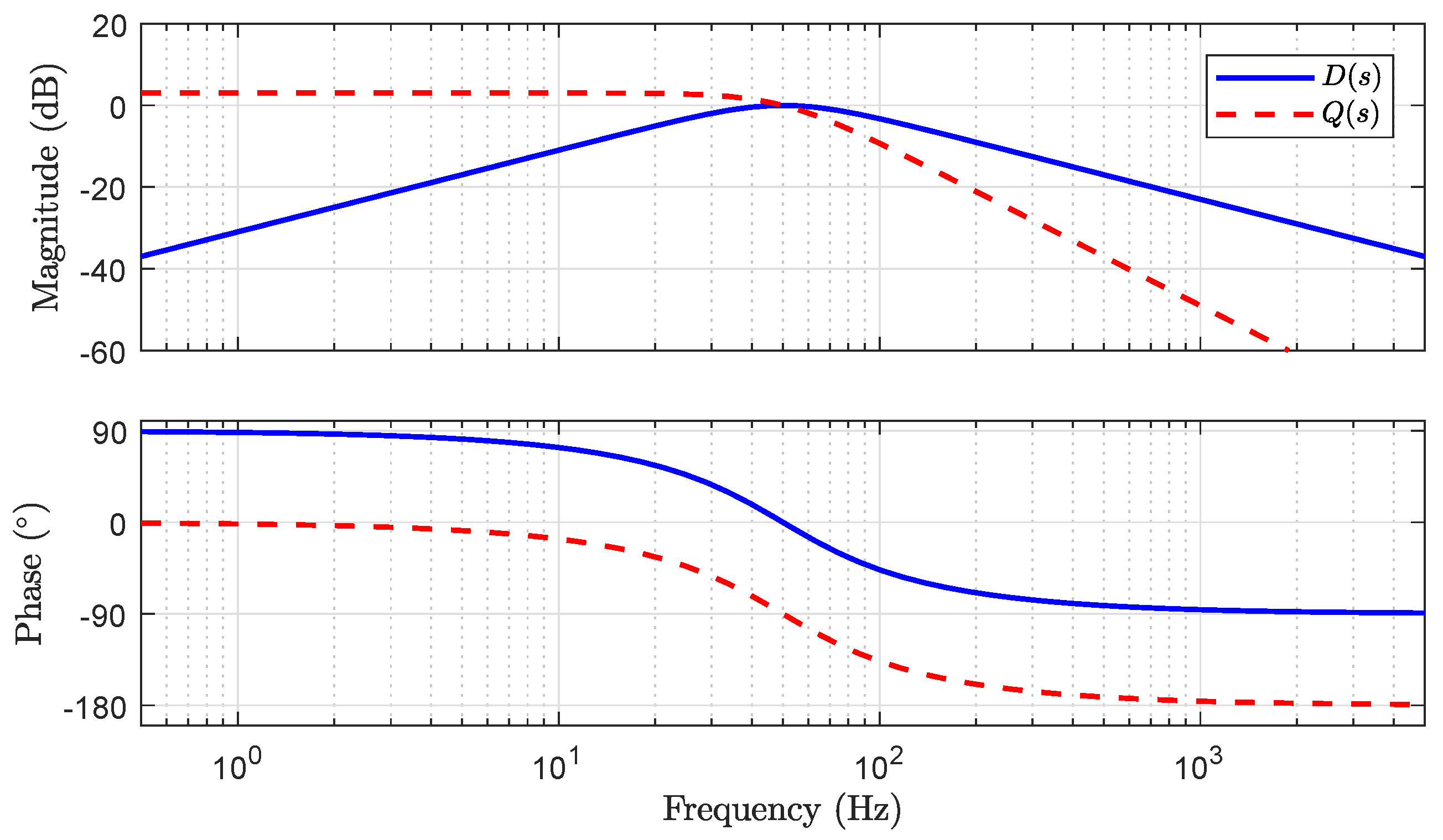
Another method is based on the single-phase enhanced PLL (EPLL). In this method, it is applied a quadrature signal generator based on the second-order generalized integrator (SOGI-QSG) to obtain a lagging 90 degrees phase shift of the input signal, offering simultaneously a filtering capability at frequencies beyond the filter central frequency [
12]. An extension of this method [
13] consists of considering a double SOGI-QSG (DSOGI-QSG), i.e., two SOGI-QSG are used to obtain the direct and quadrature signals of the alpha and beta components, respectively, for further positive sequence calculation. This method allows obtaining the positive sequence with intrinsic filtering capability. Since the DSOGI-QSG central frequency is adjusted accordingly with the PLL frequency, the DSOGI is a frequency-adaptive filter. Additionally, in [
10], it is shown that the DSOGI-PLL is equivalent to the DSRF-PLL under certain conditions; therefore, the analysis on this paper disregards the second. The DSOGI-QSG can be applied with phase tracking (PLL) or frequency tracking, becoming a frequency-locked loop (FLL).
In [
10,
14,
15,
16,
17,
18] different PLL methods, including the DSOGI-based PLL, are compared and qualified where the DSOGI is highlighted as one of the most performant. Though it does not discriminate the performance of different DSOGI-based methods and in most of the tests, it lacks numerical performance quantification.
The paper is separated into eight sections. In
Section 2 it is introduced the basic principle of work of the closed-loop PLLs, based on the synchronous reference frame (SRF-PLL). The generation of the quadrature signal, its extension to form the double second-order generalized integrator, and the extraction of the positive and negative phases sequence are presented in
Section 3. In
Section 4, it is presented the complete structure of the PLLs for synchronization with the grid-positive sequence and in
Section 5, synchronization through the frequency-locked loop (FLL).
Section 6 presents the simulation and experimental results and the respective discussion. Finally, in
Section 7, it is discussed the main chapter conclusions and the PLL implementation chosen for the thesis is justified.
2. Synchronous Reference Frame Phase-Locked Loop
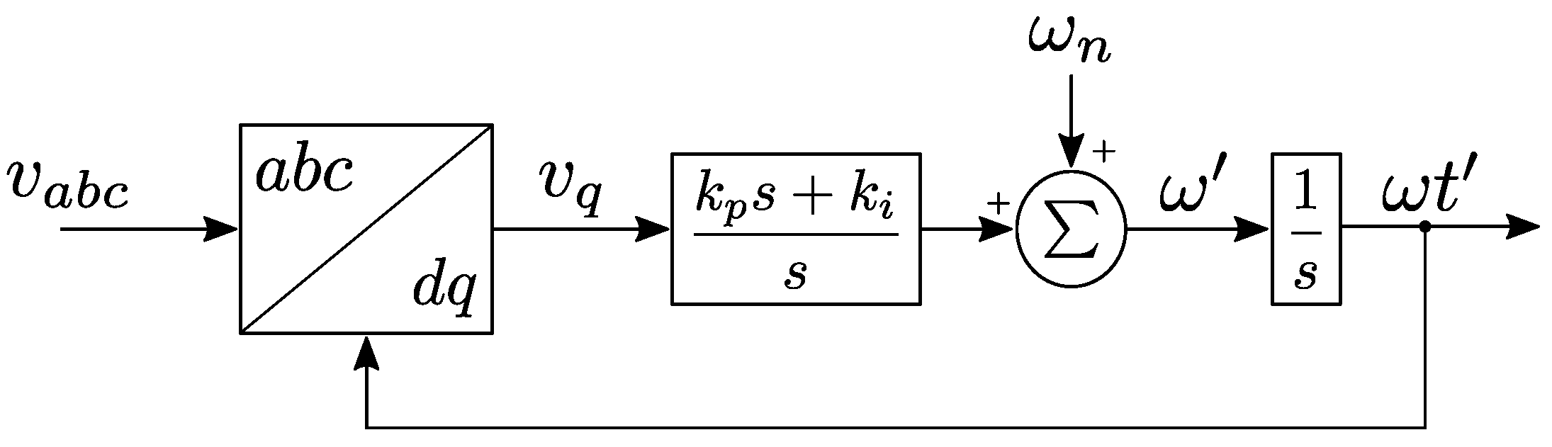
The SRF-PLL is based on the
dq0 frame, and it is illustrated in
Figure 1. The principle of operation consists of orienting the voltage vector in the
dq0 frame to be aligned with a reference phase of the three-phase voltage system. To achieve this, the quadrature component of the voltage in the
dq0 frame is controlled to zero, typically through a proportional-integral (PI) controller. It is important to notice that in the synchronous frame (
dq0 frame), all vectors rotating at synchronous speed are represented in a steady state by a constant, direct and quadrature component. The output of the PI is further integrated to obtain the phase angle that is used as feedback for the calculation of the
dq0 transformation matrix. In the steady state, the PI output and the forward compensation represent the grid frequency
.
The Clarke and Park (
1) transformation matrix, presented in
Figure 1, are in the power invariant form and aligned with the cosine of phase
. Notably, the zero component is disregarded since it does not influence the synchronization loop. Additionally, the PI gains
and
are tuned in accordance with [
3] and synthesized in Equation (
2), where
represents the filter natural (or controller) frequency,
the damping, and
the grid peak voltage amplitude.
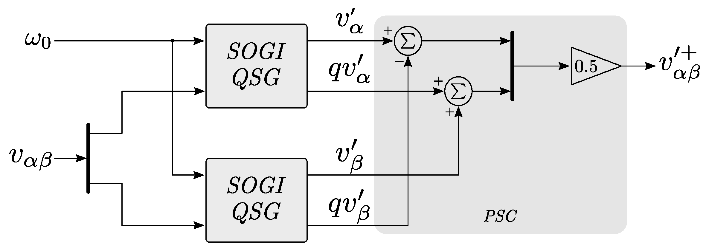
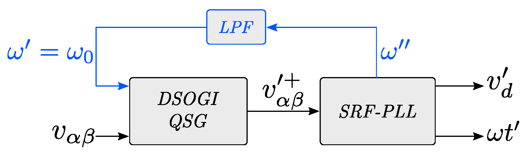
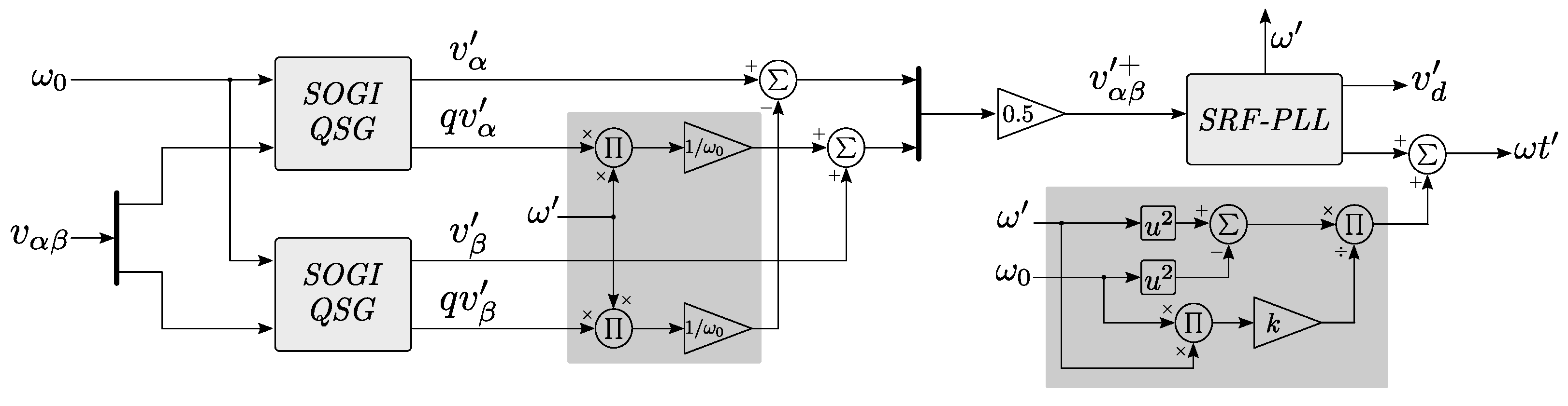
5. DSOGI Based Frequency-Locked Loop
Another approach to adapt the DSOGI-QSG center frequency
, is proposed and well described in [
22]. The author suggests an extension of the EPLL frequency adaptive structure to be applied in the SOGI-QSG. Such modifications result in the block diagram presented in
Figure 8, where
is the nominal grid frequency, and the grey area represents the gain normalization
(
9). The input error
is given by (
8), considering the SOGI-QSG nomenclature shown in
Figure 2). To highlight that the
is negative for
, zero for
and positive for
. Hence, it is possible to obtain zero steady-state errors (
) with an error integral and gain
.
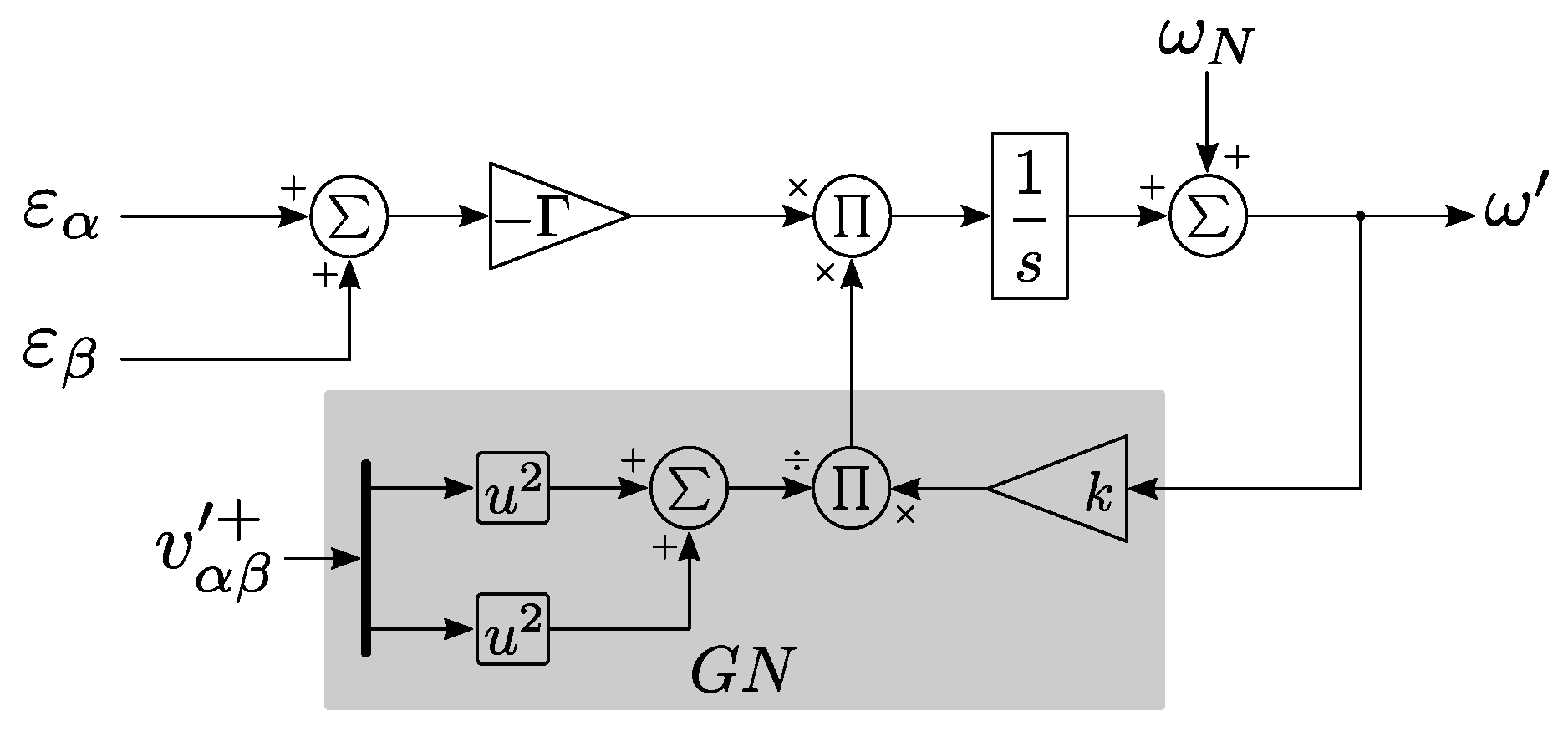
Taking into account the FLL block diagram of
Figure 8, it can be noticed that the FLL has only one tuning parameter,
, since
k is the DSOGI-QSG filter quality factor and
is a known constant. Furthermore, it is shown in [
22] that with the gain normalization, the FLL presents a first-order transfer function (
10), which allows tuning
in accordance with the desired system response settling time
.
In [
23], it is presented an improved frequency locked-loop (IFLL) that differs from the previous FLL, in a slight change on how the gain is normalized. Instead of considering only the positive sequence, the negative sequence is also considered (
11). Such modification only improves the method, when the negative sequence becomes significant compared to the positive sequence (very high unbalancing). Another method variation is presented in [
24], where a third-order generalized integrator (TOGI) is combined with an FLL for the elimination of the DC component. Such an approach is suited for single-phase systems, where the DC component is not eliminated by the Clarke transform. Additionally, any SOGI referred on this work can be turned into a TOGI for further implementation in a single-phase system.
The DSOGI-FLL (or the DSOGI-IFLL) has only two tunable parameters: the DSOGI-QSG damping
k and the FLL gain
.
To compare the synchronization of both PLL and FLL, it is suggested to add a phase estimation stage to the previously discussed FLL scheme. To achieve so, it is suggested to use the FFPS () filtered by the DSOGI-FLL to estimate the phase angle. Three different approaches are considered: zero-cross detection, SRF-PLL, and the arc-tangent function. Notice that, contrary to the PLL schemes, in the FLL, both the frequency and phase are tracked independently, despite the phase tracking accuracy being dependent on the FLL performance.
5.1. DSOGI-FLL with Zero-Cross Detection
The zero-cross detection method employed here consists of integrating the frequency estimated by the FLL, but with an angle reset at every zero-cross detected, i.e., when
or
crosses zero, the frequency integral is reset to the known angle. This way, it is possible to correct the estimated phase four times per period. Every time a zero-cross occurs, a flag is triggered (
or
) and feeds into a lookup table (LUT) to obtain the respective reset angle value accordingly with
Table 1. Though it only allows synchronizing during four instants per wave period, this method is simple with a low processing demand, though it may lead to significant phase deviations during transients. This method does not add tunable parameters to the DSOGI-FLL.
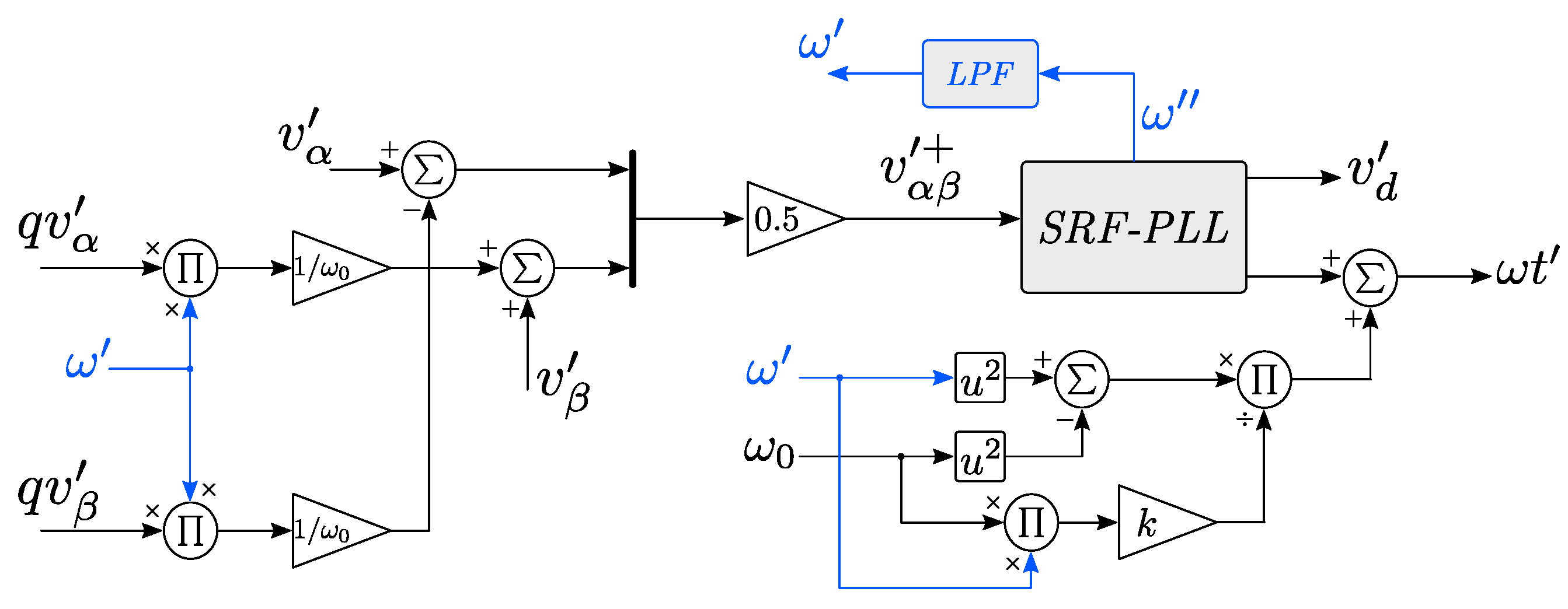
5.2. DSOGI-FLL with SRF-PLL
The SRF-PLL can be added to the DSOGI-FLL to further estimate the phase frequency. Different from the PLL methods, in the FLL, the PI dynamics of the SRF-PLL do not influence the positive sequence extraction since the center frequency feedback of the DSOGI-FLL does not depend on the PI but on the FLL block diagram instead.
This scheme is here called the DSOGI frequency and phase-locked loop (DSOGI-FPLL). The method adds two tunable parameters to the original DSOGI-FLL ( and ), resulting in a total of four tunable parameters.
5.3. DSOGI-FLL with Atan2
The last considered method consists of calculating the arc-tangent of
to obtain the respective angle at any time instant. To reduce the processing burden associated with the typical arc-tangent methods, the fast arc-tangent suggested in [
25] is employed. The proposed function is implemented through a LUT (or array) with limited angle representation, i.e.,
or
. To extend its operation for the four quadrants, the functional properties (
12) and (
13) are considered.
6. Results and Discussion
To compare the different SOGI-based PLL performance under severe grid conditions of a weak grid, several simulations are performed in Matlab/Simulink. Furthermore, all aforementioned methods were implemented in the discrete-time domain with a sampling rate of 10 kHz to emulate the micro-controller behavior. Discretization was performed considering the forward Euler integration method.
The performed tests are divided into three different subgroups: unbalancing and harmonics (test
), frequency and phase jumps (test
), and voltage sags (test
). However, in the last two, harmonics and unbalancing are also considered but with a smaller impact. In
Table 2, it is shown the harmonic content considered in the different tests as a percentage of the FFPS voltage.
The grid voltage is generated directly from pre-defined positive and negative sequences, while harmonics are posteriorly added. Hence, at any instant, it is possible to know the exact frequency, phase, and magnitude of the fundamental positive (and negative) sequence and the harmonics magnitude.
Additionally, it is considered that the PLL is locked when the estimated frequency reaches a steady state. Therefore, if both the FLL and PLL dynamic responses present the same frequency settling time, it is possible to carry a fair comparison between the methods. Hence, PI was tuned (
2) considering
rad/s and
, while the FLL gain was tuned (
10) with
. The SOGI damping, in all different methods, was set as
. The tuned gains are summarized in
Table 3.
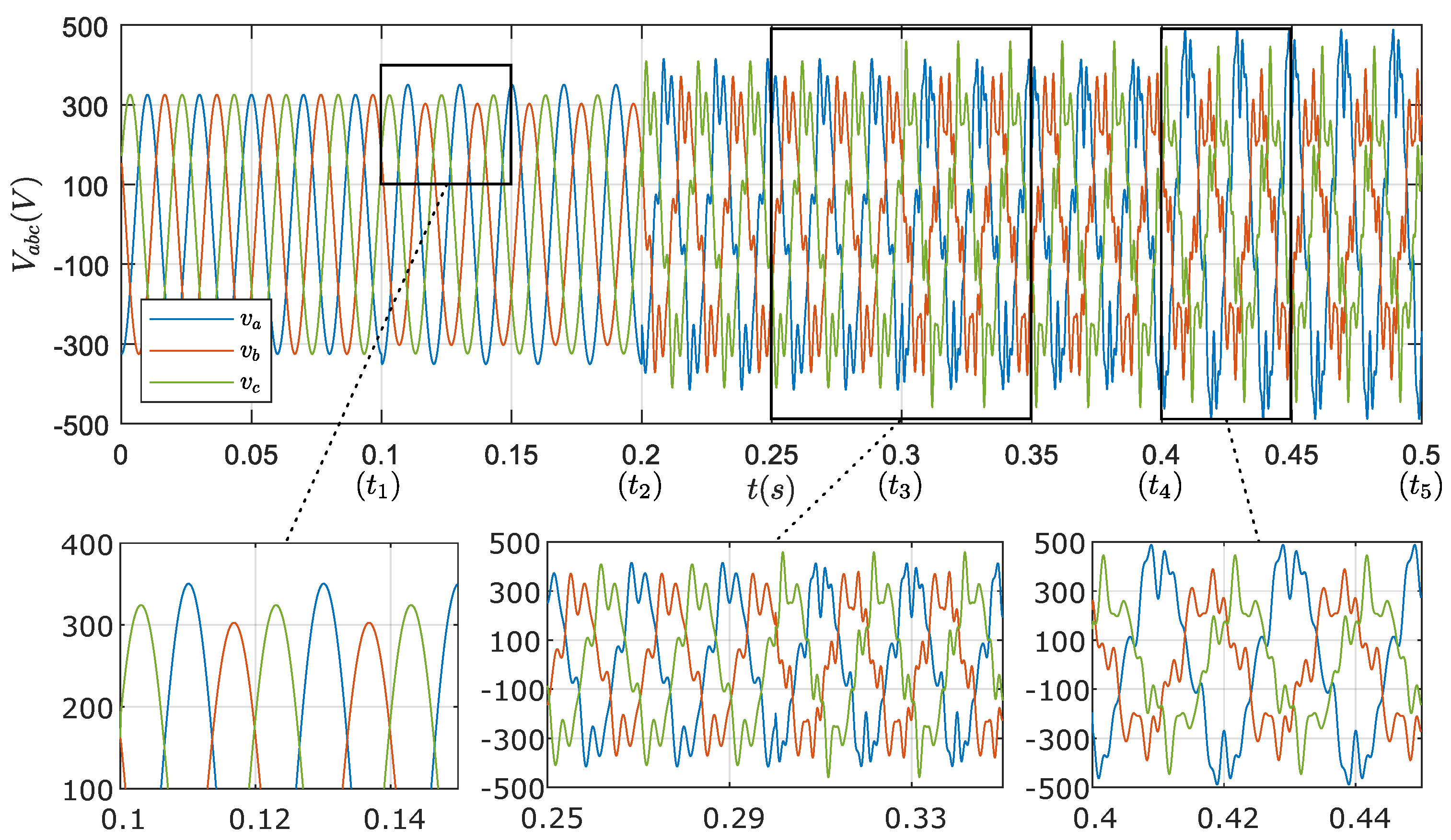
6.1. Test —Unbalancing and Harmonics
This test considers balanced three phases (positive sequence only) at 50 Hz, with all the methods already in a steady state at the simulation start. Unbalancing is achieved by injecting a negative sequence component, followed by harmonics with an amplitude, as presented in
Table 2. Moreover, for the phase estimation, the results in this test are first applied to the FLL (DSOGI-IFLL) and further compared with the PLL (DSOGI-PLL and FFDSOGI-PLL).
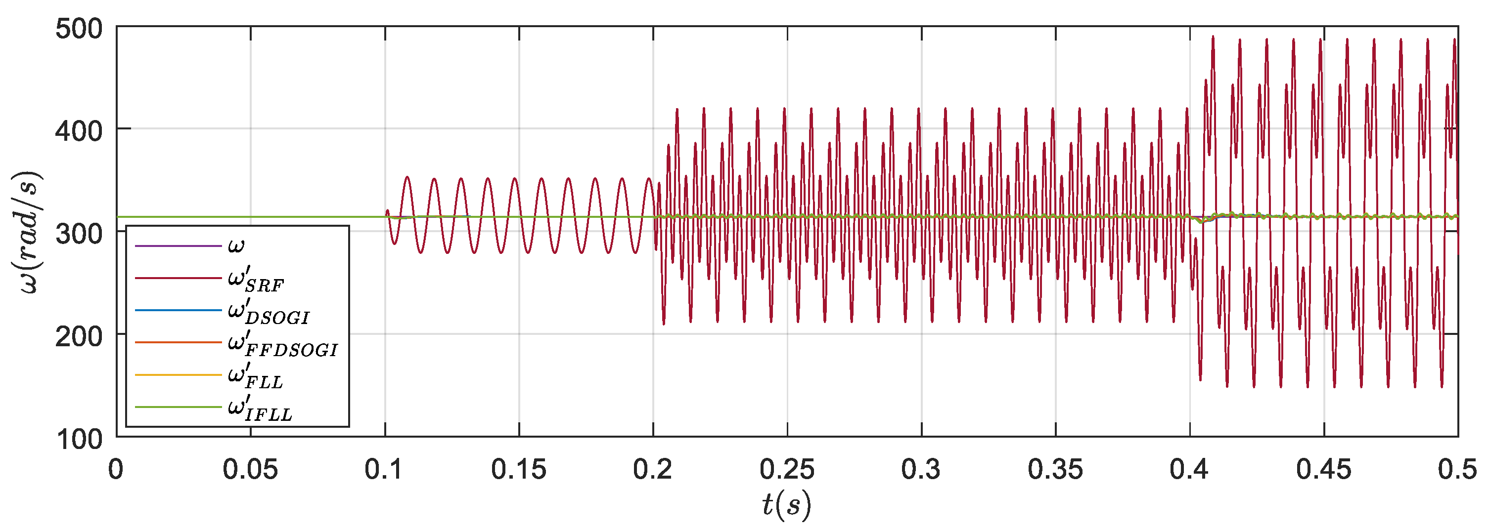
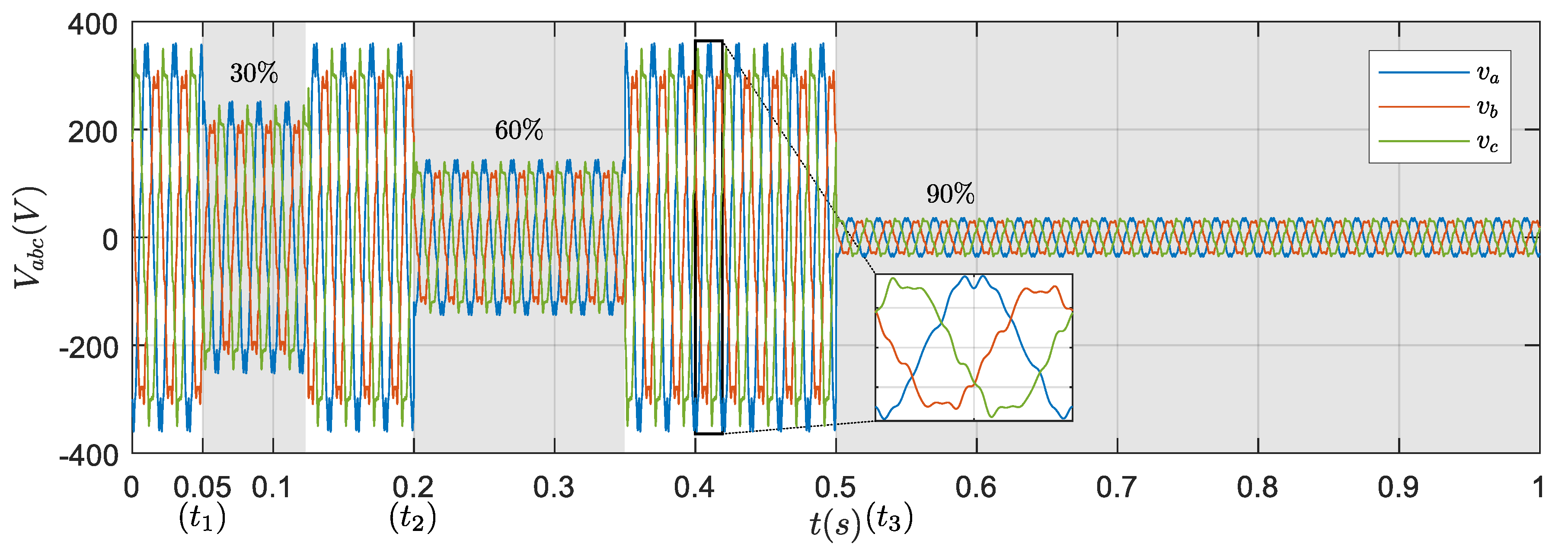
The analysis of the three-phase voltages are illustrated in
Figure 9, where
to
are the time instants that mark the added changes to the subsequent conditions listed in
Table 4. The estimated frequency
and the respective errors (
) are illustrated in
Figure 10 and
Figure 11, respectively. In
Figure 10, it can be noticed that all methods remain near the nominal frequency with the exception of the SRF-PLL. Its performance is significantly poor when facing unbalanced conditions and further deteriorates when high low-order harmonics are present in the three-phase voltage. For these reasons, the following analysis disregards the SRF-PLL and justifies the need for methods capable of extracting the FFPS.
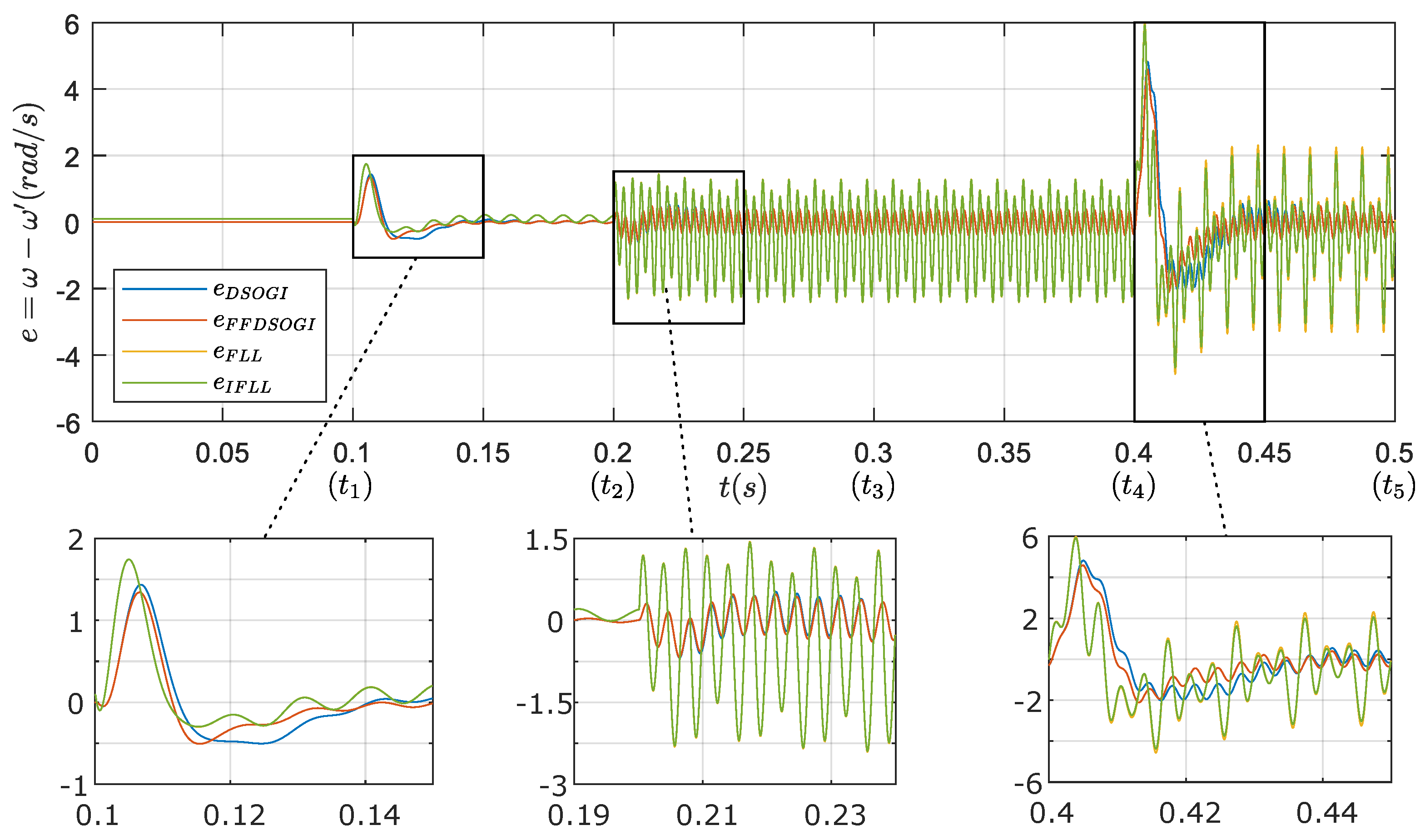
In
Figure 11 it is noticeable that the DSOGI and FFDSOGI (PLL) presents similar behavior, both with lower estimated frequency steady-state oscillations when compared with the FLL methods. Furthermore, both FLL and IFLL perform very similarly, mostly until
, where the negative sequence is reduced. After
, unbalancing is more noticeable and the IFLL presents lower oscillations than the FLL, though such a difference may be neglected. To allow a quantification analysis of the results, in
Table 5, it is presented the root mean square error (RMSE) as a measure of the error oscillations, and the mean error (ME) as its DC value during steady-state stages. In
Table 5,
and refers to the FFPS voltage waveform time period.
Analyzing data from
Table 5, it can be noticed that under ideal conditions
the FLL and IFLL present a higher steady-state error (ME) when compared with the DSOGI-based PLL structures, though under such conditions, all methods perform very well. With the introduction of the three-phase unbalancing and harmonics, oscillations are more noticeable in the FLL methods than in the PLL. An interesting behavior of the FLL methods is in the change of the steady-state frequency ME with the changes in grid conditions. Observing the integral error of the FLL, it is concluded that the integral error gain is high enough to guarantee zero steady-state error, which indicates that the small ME is caused by the FLL structure, particularly in the way that the error
is generated for adapting the frequency.
Since both the FLL and IFLL performance are similar, only the IFLL is considered in the following performance evaluation.
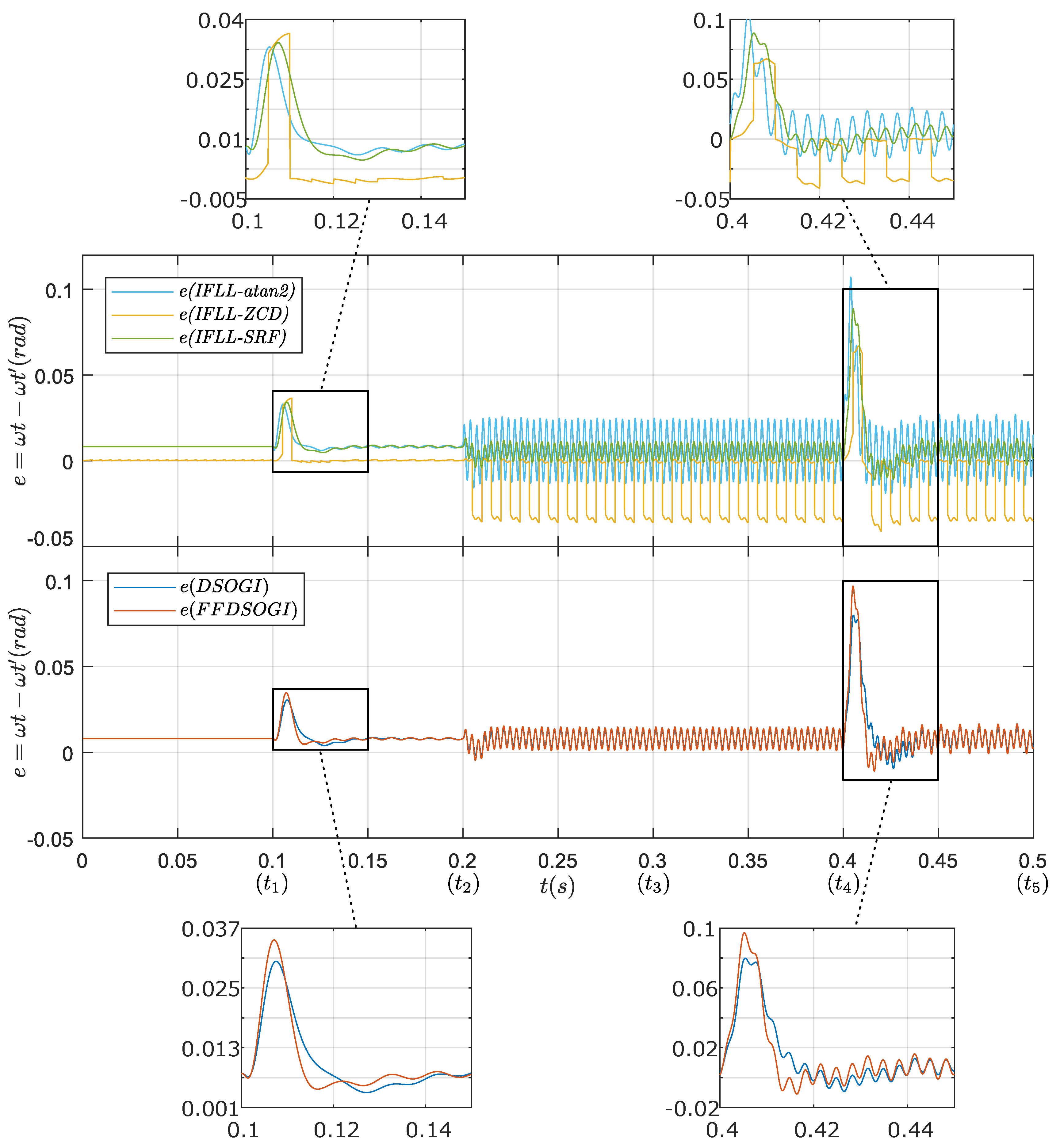
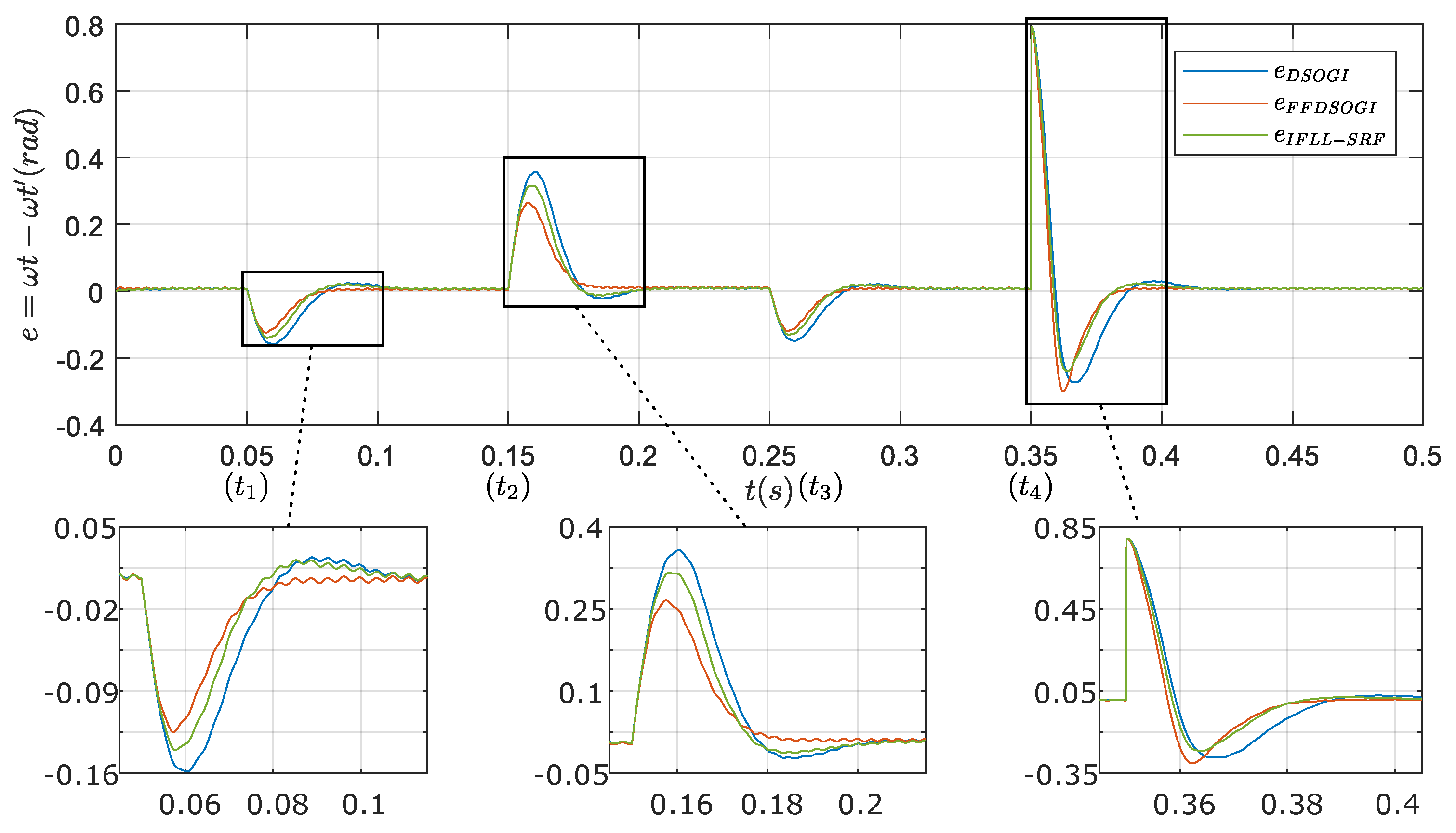
In
Figure 12, it is presented the errors obtained for the phase estimation
. Note that the different methods presented in
Section 5 for phase estimation are applied to the IFLL (FLL is not shown since it presents similar results). Furthermore, the RMSE and ME were obtained under steady-state conditions for the same intervals of
Table 5 and are shown in
Table 6.
Through analysis of
Figure 12, it is clear that the IFLL-SRF results in the most stable angle estimation when compared with the IFLL-atan2 and IFLL-ZCD. Hence, the non-linearity on phase reset at every grid period quarter (IFLL-ZCD) and the high oscillations in the IFLL-atan2 indicate that the
components resulting from the DSOGI-FLL are not strictly sinusoidal nor do they present a phase difference of exactly
. Such distortions are introduced mostly by the low order harmonics as already concluded before in the frequency analysis. In [
7,
23], it is suggested to add multiple DSOGIs tuned at different harmonic frequencies for the elimination of the respective low order harmonics; however, such an extension is not explored in this paper.
The PLL methods perform very similarly as expected, though the DSOGI-PLL outperforms all the other methods in terms of overall performance as it can be concluded by analyzing the RMSE during steady states, presented in
Table 6.
For the test conditions, it can be concluded that the performance of both PLL methods is superior to the FLL. Where the FFDSOGI presents the best results in frequency estimation and the DSOGI in the phase angle, both perform very similarly in both estimations. Despite the differences, as far as harmonics and unbalancing conditions are considered, all methods based in the SOGI-QSG show great performance under unbalancing conditions and good harmonics filtering capability.
To qualify the obtained results for the different methods during test , it is considered only the steady-state oscillations (RMSE). During test , the ME remains practically constant for both frequency and phase estimations, making it more meaningful to analyze the ME with the results obtained during test . Furthermore, the RMSE is applied to the frequency estimation since in the case of the phase angle estimation, the differences can be disregarded. The final classification is shown later in Table 12, where the mark is defined by the averaged ratio of the method RMSE by the minimum RMSE obtained for the different grid distortion intervals.
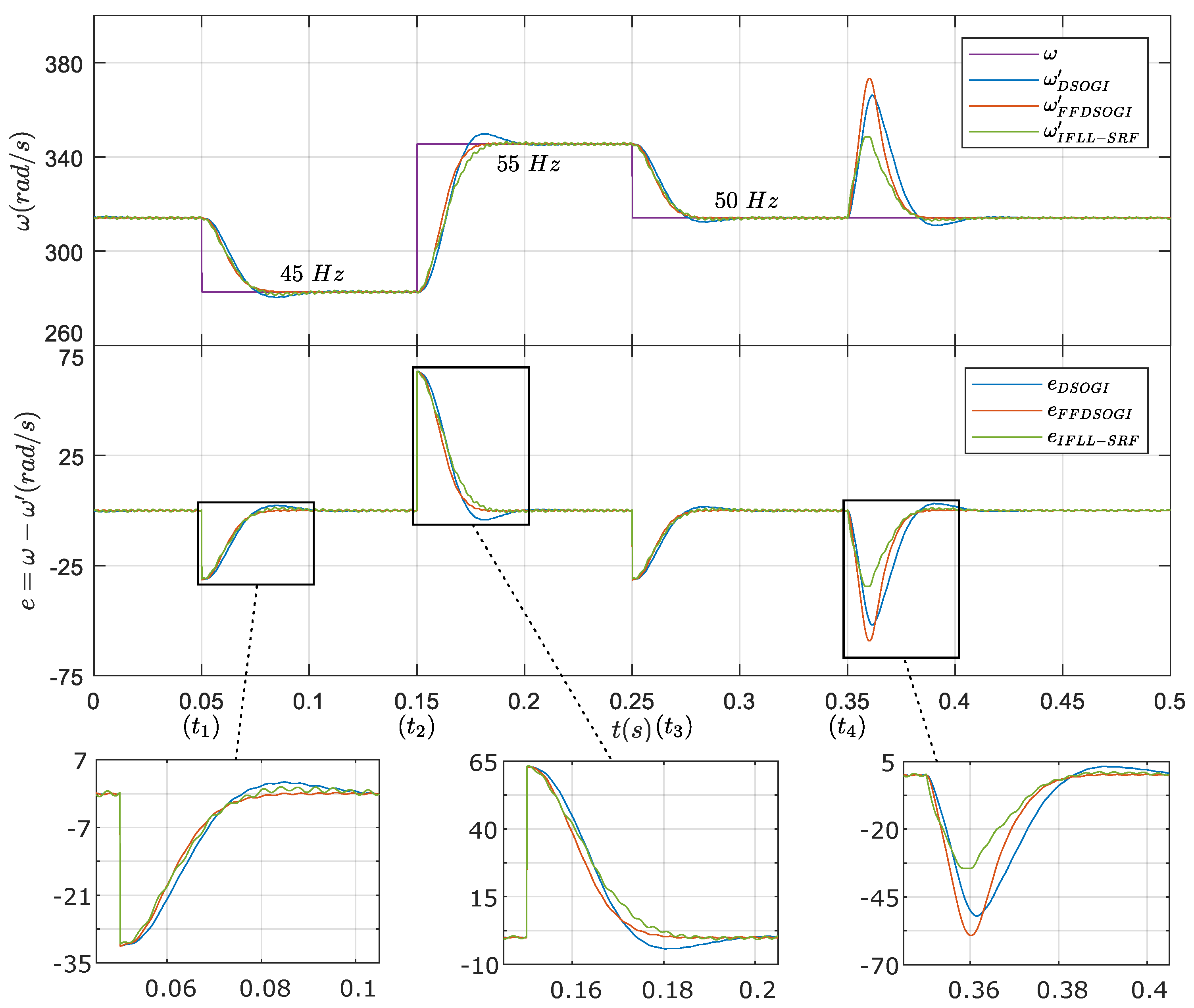
6.2. Test —Frequency Steps and Phase Jump
Test
consists of applying frequency steps followed by a phase jump. The test, as already stated before, also considers unbalancing and low-order harmonics in accordance with
Table 2. The frequency and phase profile is equally applied to the three phases and is summarized in
Table 7.
The results obtained for the estimated frequency and respective frequency errors during test
are shown in
Figure 13.
In
Figure 13, the steady state of the different methods is coherent with the results obtained during test
, and, therefore, it is not analyzed again. The frequency steps at
and
are the same (
), and it can be seen that the transient response of the FFDSOGI and IFLL are very similar, both in terms of overshoot and settling time. During this step, the DSOGI takes almost
more to reach the steady state. At
occurs the biggest frequency step (
) and during this transient, the FFDSOGI presents a slightly faster response. Finally, at
occurs the
phase shift, and the results, in terms of the response time, follow the same behavior as during
. Nevertheless, the IFLL presents significantly less overshoot than other methods, which indicates that the FLL scheme is less sensitive to phase jumps when compared with the PLL.
To evaluate the performance in terms of phase estimation, the results in
Figure 14 are presented. In terms of phase estimation, during frequency step changes, the differences are more obvious, where the FFDSOGI performance is better than the others, both in terms of overshoot and settling time. The FFDSOGI reaches its steady state in
s, with the following taking
s more. Still, during the phase jump, the FLL presents less overshoot and takes the same time to reach the steady state, which corroborates the estimated frequency results.
In
Table 8 and
Table 9, the results are summarized for the methods that presented the best performance during test
. In
Table 8,
is the overshoot and
the settling time. In
Table 9, it is shown the ME for estimation of the steady-state frequency and phase at different grid frequencies.
Based on the results summarized in
Table 8 and
Table 9, the final classification is presented later in Table 12. The classification is based in the average ratio of each evaluated value with the minimum value obtained during that test for the different conditions. Hence, the best result corresponds to the smaller classification value
.
6.3. Test —Voltage Sags
During test
the grid frequency is kept constant (nominal value), while harmonics and unbalancing are the same as those applied in test
(
Table 2 and
Table 4). Hence, the changes applied during the present test focus on the voltage amplitude, i.e., the sags are applied to the symmetrical voltage components and also the harmonics.
The voltage sags periods and amplitudes are summarized in
Table 10 and the resulting grid voltage waveforms are shown in
Figure 15.
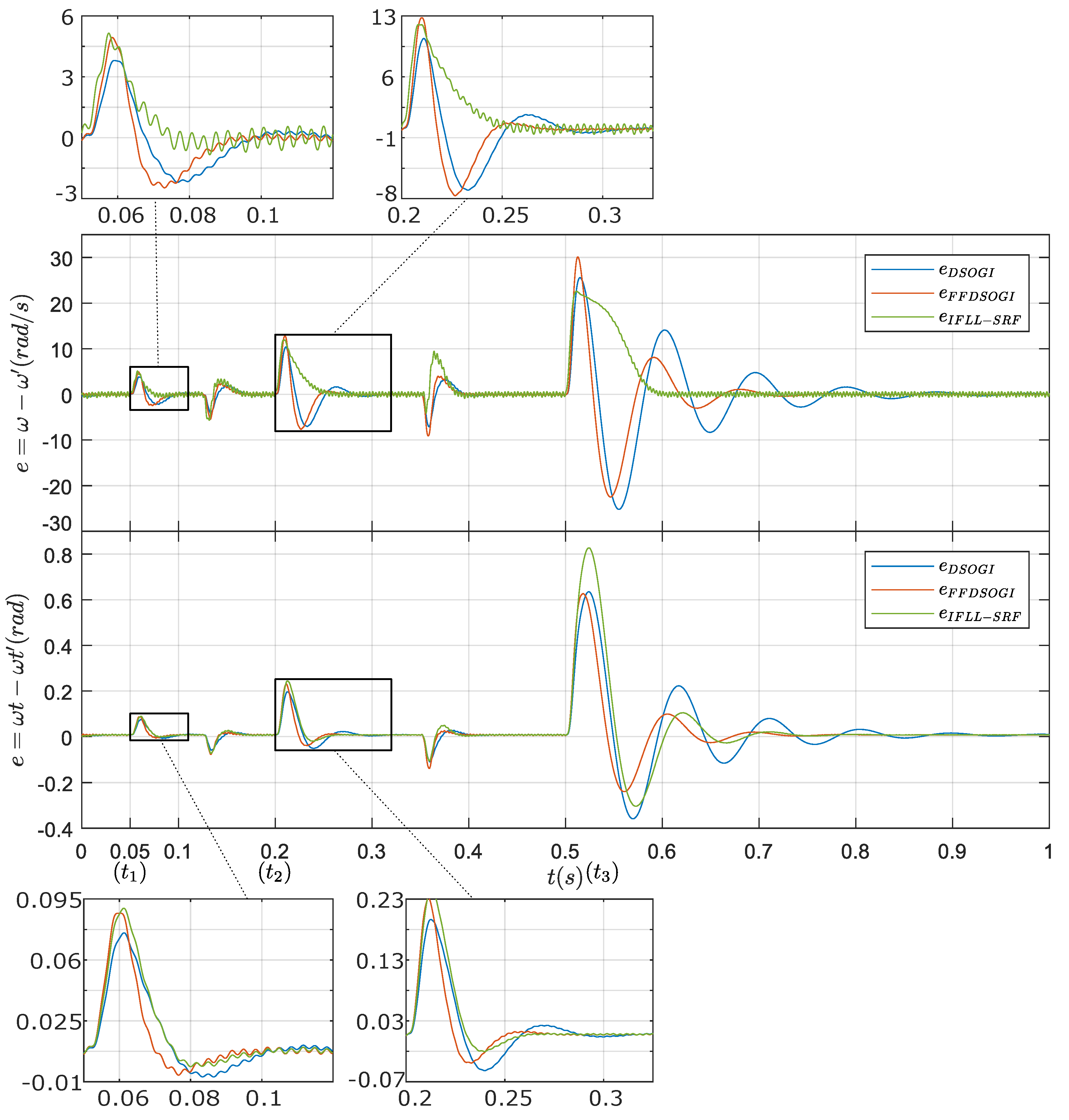
The errors associated with frequency and phase estimations, obtained during test
, are shown in
Figure 16, where the top plots refer to the frequency and the bottom ones to the phase.
Analyzing the frequency dynamic response of
Figure 16 allows concluding that all methods respond very similarly to the
voltage sag (
). During the
voltage sag (at
), both FFDSOGI and IFLL-SRF also perform with the same settling time, despite the first response with larger oscillations. In the same interval, it is noticeable the weaker performance of the DSOGI, which takes ≈20 ms more to reach a steady state. The
voltage sag is the perturbation with a higher impact of all the analyzed tests, where it can be seen the long settling time of both FFDSOGI and DSOGI, with both taking, respectively, 200 ms and 350 ms to reach a steady state. On the other hand, the IFLL-SRF presents a significantly faster response time, taking 100 ms to reach the steady state.
In terms of phase dynamic response, the results are coherent with the aforementioned comments for the estimated frequency. The only exception is during (), where the IFLL-SRF presents a phase response, similar to the FFDSOGI, of ≈200 ms.
The summary of the voltage sag results is presented in
Table 11, where the steady-state ME is not shown since it remains approximately constant for all methods.
6.4. Tests Benchmark
Taking into account
Table 5,
Table 8,
Table 9 and
Table 11, classification
Table 12 is presented. For classification purposes, the marks were calculated by considering the ratio of the averaged registered values (per method of each test transition) by the minimum average obtained from all tests for each test transition. Therefore, the best result (minimum value) for each test/transition is
and the choice of the suitable method should be based on the minimum classification value obtained. The table classifications are divided into two categories (frequency and phase), where for each category, the methods are classified in terms of the steady-state performance
SS (RMSE or ME), dynamic response to frequency step changes
, phase jumps (
), and voltage sags
(evaluating both the overshoot and settling time). It can be noticed that the steady state is based only on the average of the RMSE for the frequency and the average of the ME for the phase angle estimations (both from test
). The choice of the steady-state error indicators was based on its significance, i.e., the RMSE in the case of the frequency, and ME in the phase estimation.
For the grid-following operation with the main grid (strong grid) sudden changes are not expected, such as voltage sags or frequency steps, since the grid voltage transients are slow and smooth when compared with the converter and PLL dynamics. Hence, in this case, it is recommended to consider the steady-state phase and frequency estimation (RMSE and ME) and the MCU burden as the selection criteria. In such conditions, the DSOGI-PLL is the best choice by a marginal difference when compared with the FFDSOGI (selection based on the method simplicity and MCU execution time of Figure 23). The IFLL is only recommended if fast-tracking of frequency is important during voltage sags or phase jumps, where mostly because of its gain normalization, a smoother and faster response is achieved when compared with the other methods but at the cost of a higher MCU burden. Such a requirement can be considered in power converters operating with reactive power compensation in inductive weak grids. The FFDSOGI outperforms the other methods in the overall results of the test, making it the most suitable choice when uncertain conditions are expected. The only constraint with high impact in its selection is related to the grid frequency variation, which must be small ().
Through the presented classification table, it is possible to apply weights to the different marks and select the best method based on the minimum value obtained.
As an example, in this paper, the choice of a PLL to be applied on a power converter control loop is considered, operating in a low-voltage microgrid as described in [
27]. In such conditions, the grid can be either weak (island) or strong (grid connected). In the grid connected (strong grid) condition, the most important requirements are as discussed in the previous paragraph. When operating in island mode (weak grid), the lack of inertia may result in the occurrence of any of the earlier mentioned perturbations. Since the phase angle estimation is the crucial variable of interest, in the operation of the power converter, the following weights (applied to each component in parenthesis) are suggested:
Phase angle steady-state estimation is of high importance since controllers are designed to operate in the SRF ();
Frequency should be according to EN 50438, i.e., deviance inside the limit ;
Phase jumps may occur during re-connection with the main grid ();
Voltage sags may occur during overload conditions or heavy-load connection ();
Low MCU processor burden ().
Following the marks and listed criteria in
Table 12, the best choice is FFDSOGI-PLL (
pts), followed by DSOGI (
pts), and IFLL (
pts).
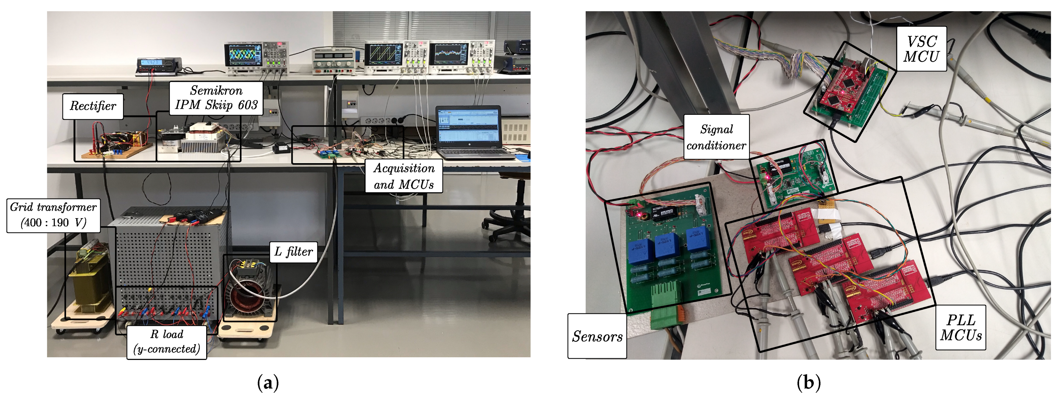
6.5. Experimental Results
To evaluate and confirm the synchronistic performance of the methods discussed in the previous section, a voltage source converter (VSC) is configured to generate a local grid voltage (instead of a DAC board) so that the switching EMI can be present in the measurements. The VSC operates in an open-loop as a programmable voltage source with a filter inductance supplying a resistive load that is y-connected. Hence, it is possible to generate any three-phase voltage through VSC modulation signal manipulation.
Additionally, voltage measurements are taken at filter output; therefore, the modulation phase angle leads the measured phase voltage, due to the load angle. As a consequence, the estimated phase angle presents a DC error resulting from the load angle when the modulation phase angle is taken as reference. The resulting setup is presented in
Figure 17. The harmonics injected in the modulation are also adjusted so that the voltage, measured at inductance output, contains the harmonics as indicated in
Table 2.
For evaluation of the methods, three identical MCUs (Infineon XMC 4500) were programmed, each with a different method. The sensed three-phase voltage was fed into each of the MCU boards and the two DACs available per board were tuned for further evaluation of the results. The PLL MCU DACs generated signals according to the estimated frequency and phase angle of each method and were compared with the VSC MCU modulation frequency and phase. The generated voltages were limited below , though MCU readings were amplified by a factor of 3 so that the measured voltage approached near nominal grid conditions. Notably, the presented setup does not allow to apply steps as applied during the simulation, due to the time constant.
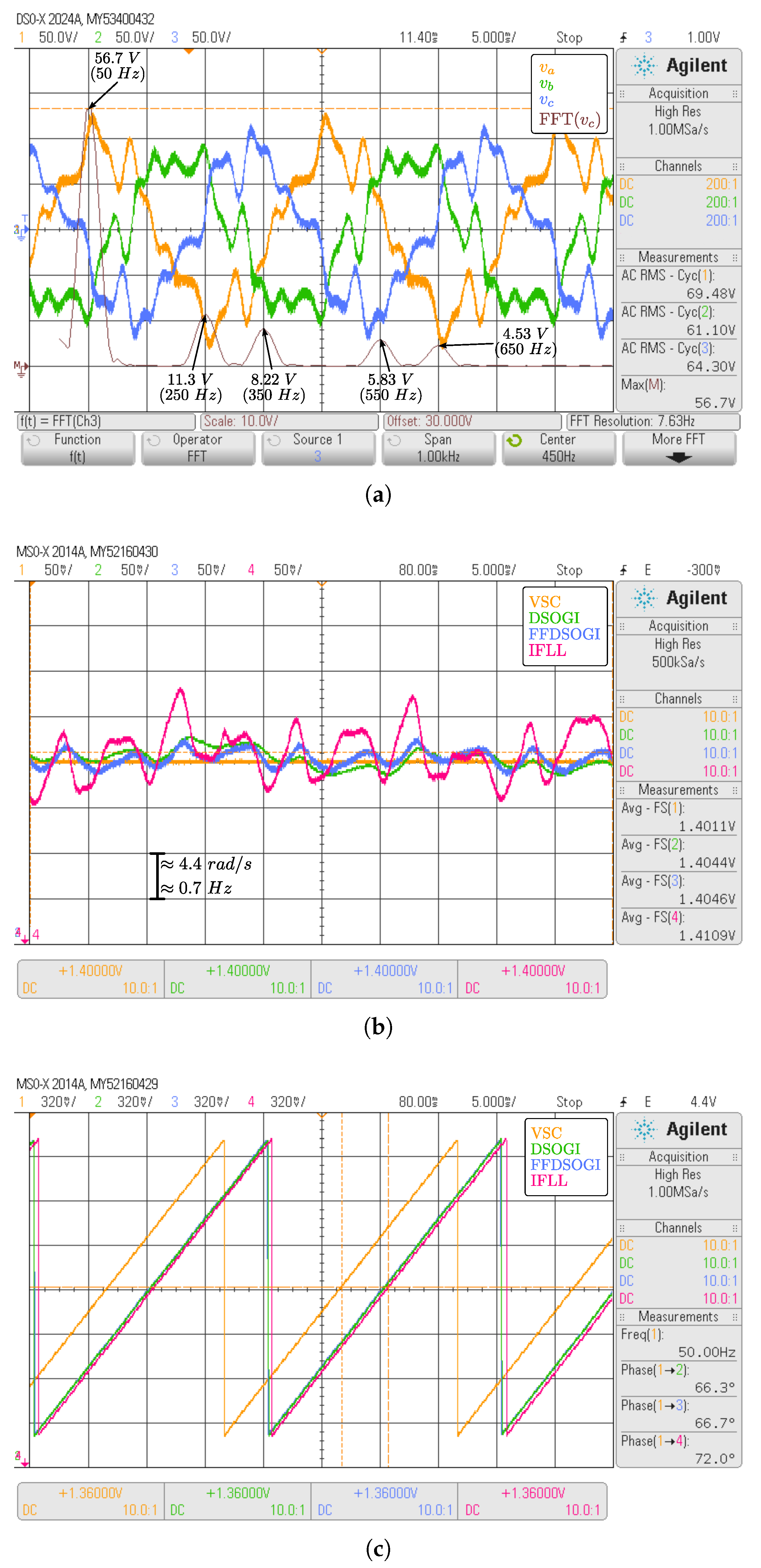
In
Figure 18 are shown the results obtained for test
considering conditions similar to
of
Table 4. In the figure, it is shown the voltage waveforms at filter inductance output with unbalanced phase voltages and harmonic content, measured through the oscilloscope FFT function.
Analysis of the results obtained for test
allows concluding that, as discussed in
Section 6.1, the DSOGI and FFDSOGI methods perform very similarly in terms of frequency estimation. The IFLL presents higher oscillations than the other two, though such differences are not as noticeable in practice as the ones obtained during simulation. The phase estimation of the IFLL presents a higher ME (DC error) than the other methods, as also discussed in
Section 6.1. Despite not being noticeable in
Figure 18, the steady-state phase estimation oscillations are identical in all three methods. Such a fact was concluded by monitoring the PI outputs of all methods.
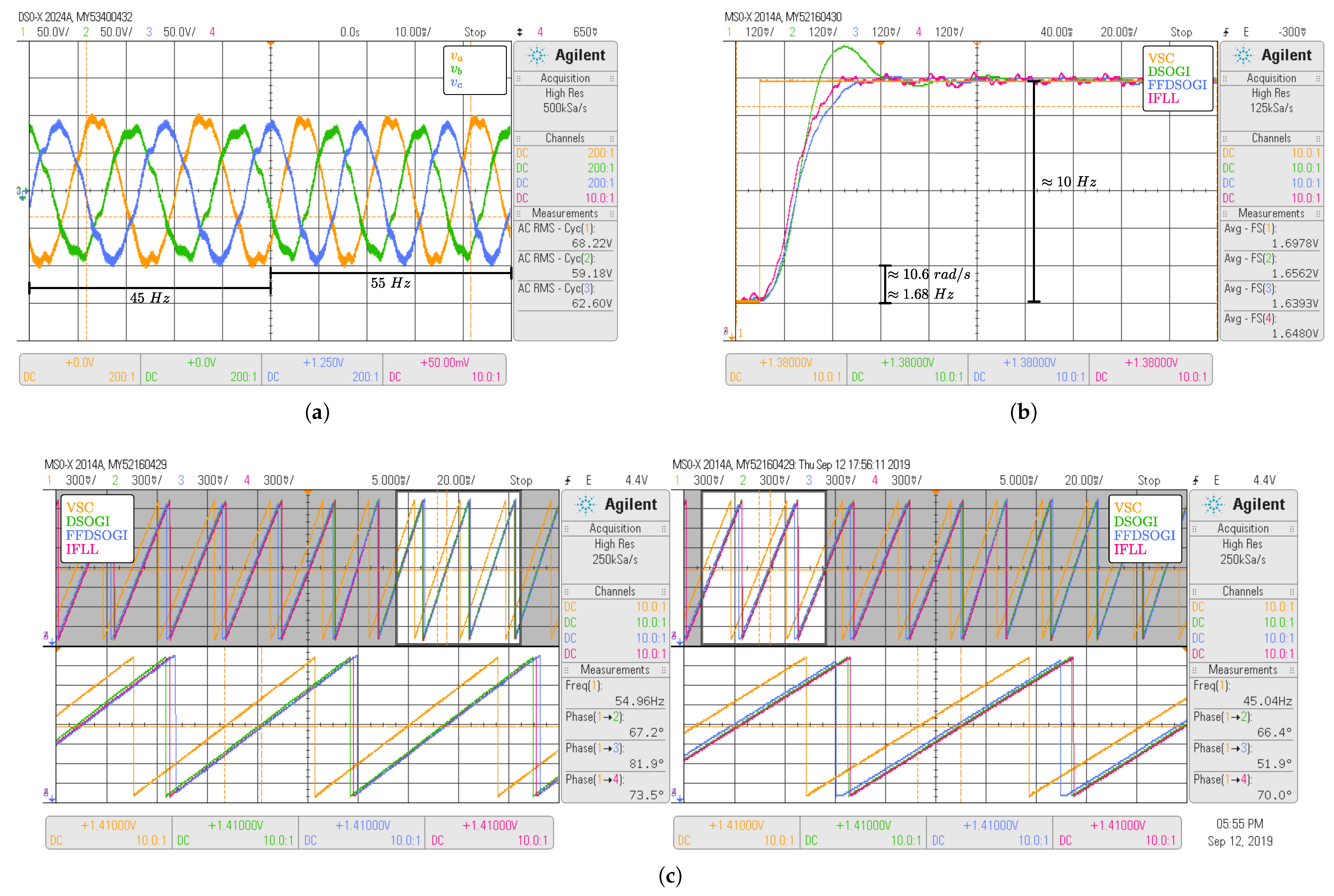
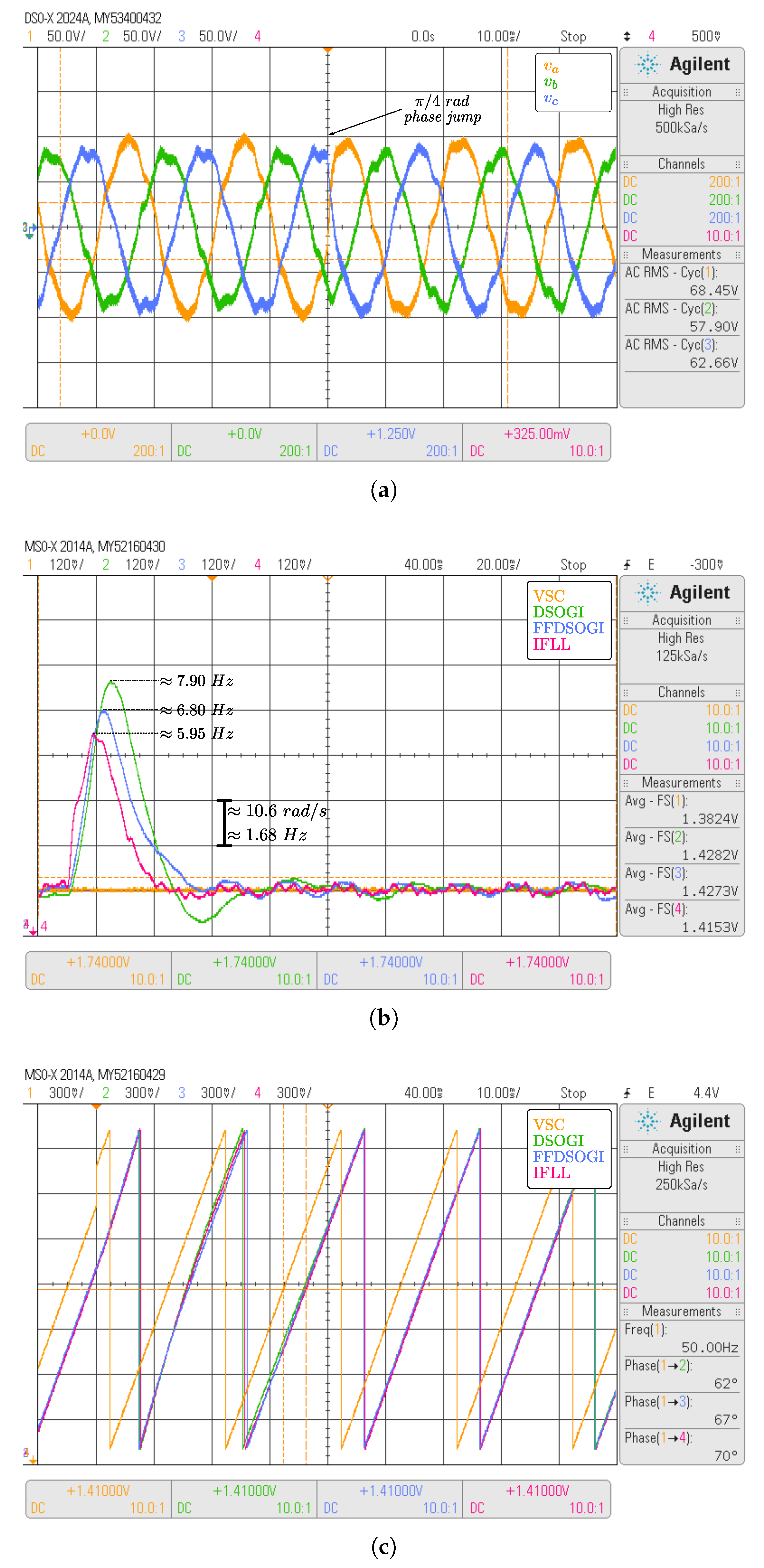
For test
, it was applied a frequency step (
), as shown in
Figure 19, and a phase jump of
at nominal frequency (
Figure 20). Additionally it is shown in
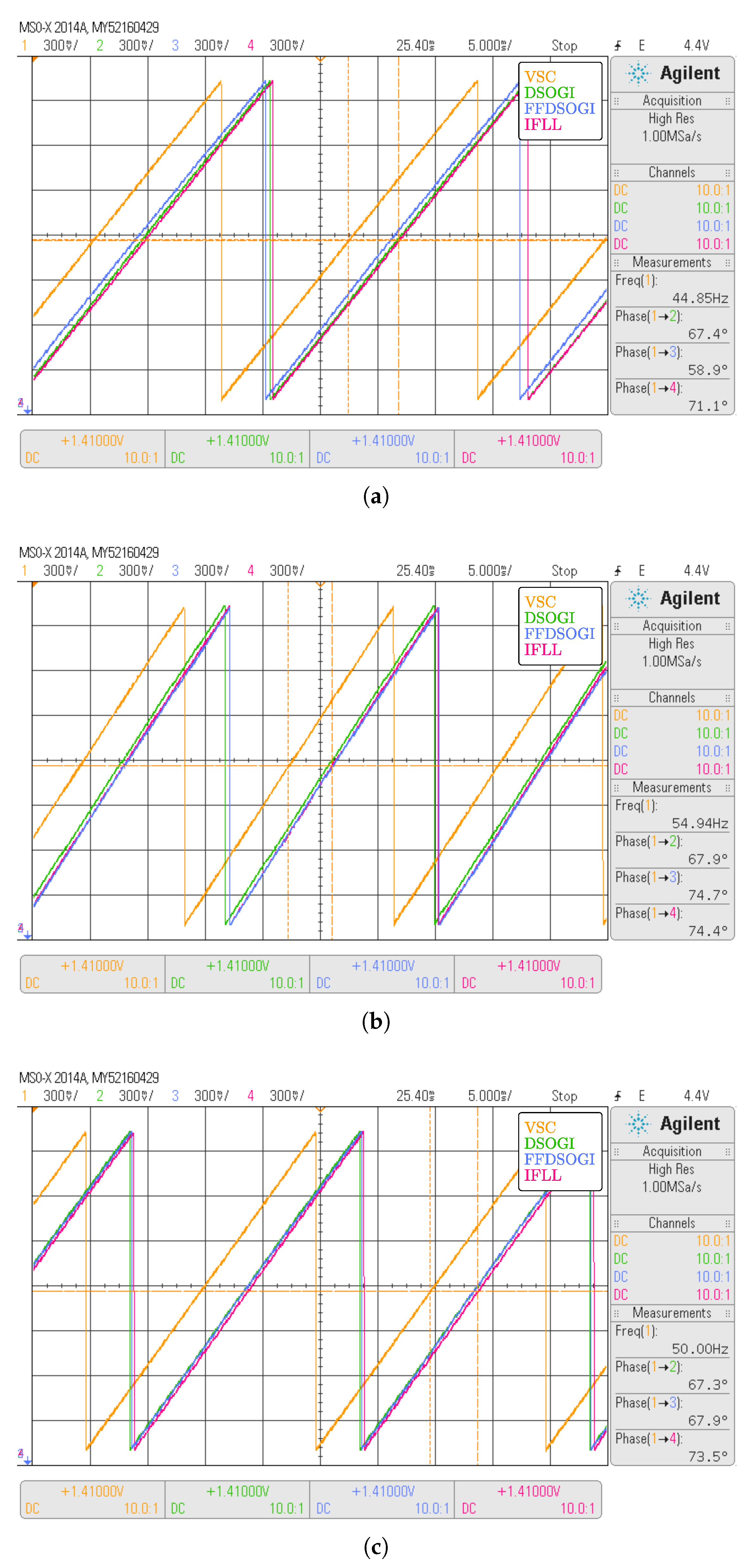
Figure 21 the estimated angle in a steady state for both limit frequencies.
The obtained results agree with the discussion in
Section 6.2. The estimated frequency of both tests (
Figure 19 and
Figure 20) follows the results already discussed. The only exception is for the phase estimation by the FFDSOGI during limit frequencies, i.e., there is a DC error of the phase estimation that changes depending on the frequency. Such behavior is justified by the method linearization for the phase estimation and can be visualized in
Figure 21 by checking the change in the phase difference between the modulation phase angle (VSC) and the FFDSOGI.
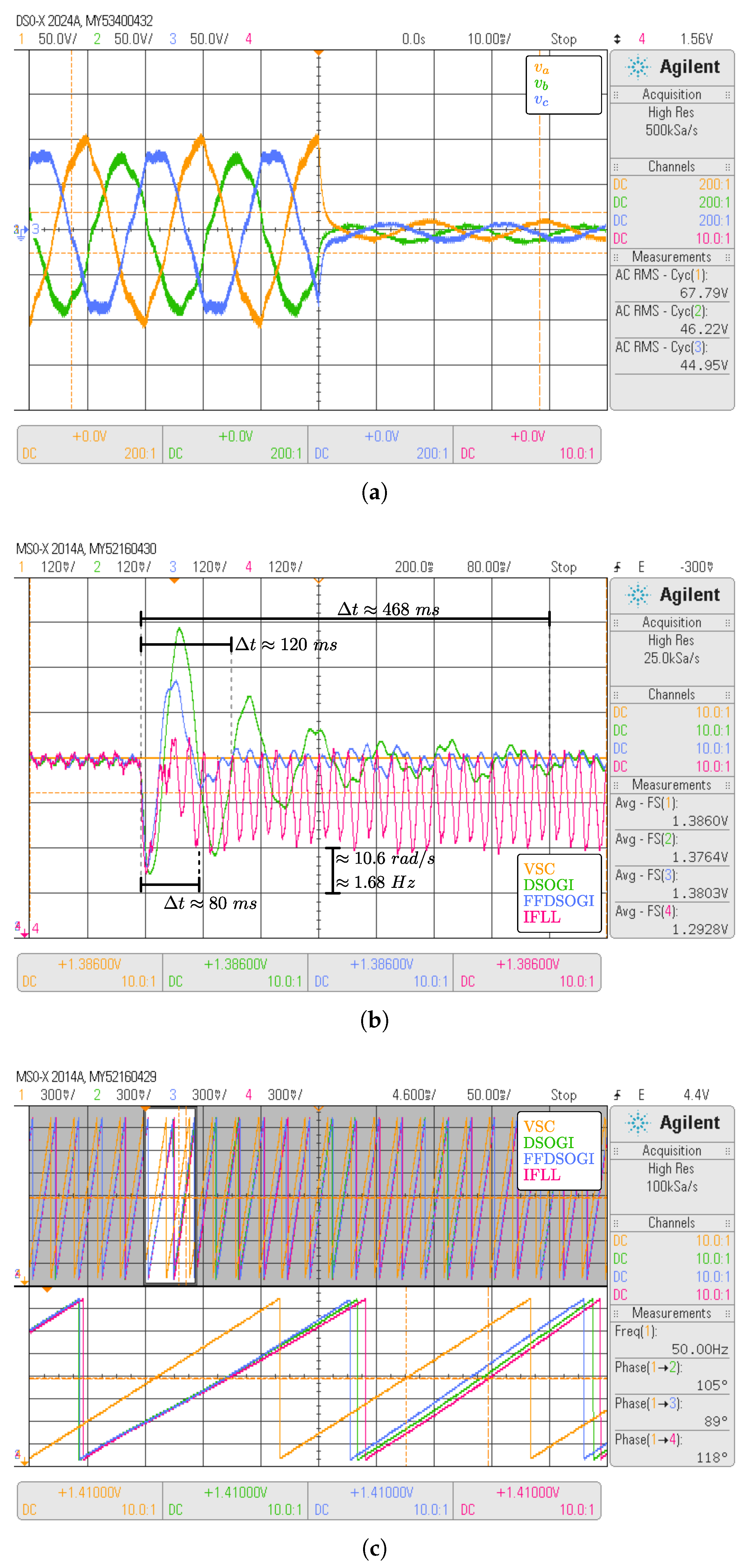
For the voltage sag of test
, a
sag is applied since it corresponds to the simulated worst case, and the respective obtained results are presented in
Figure 22.
From
Figure 22, it can be noticed that the IFLL is the method that responds faster, although it presents significantly higher steady-state oscillations and a change in the average frequency estimation value. The FFDSOGI takes
more than the IFLL to reach a steady state, though it presents significantly fewer oscillations and the steady-state average error can be neglected. The DSOGI behavior follows the FFDSOGI one with the difference of taking longer, by
, to reach a steady state.
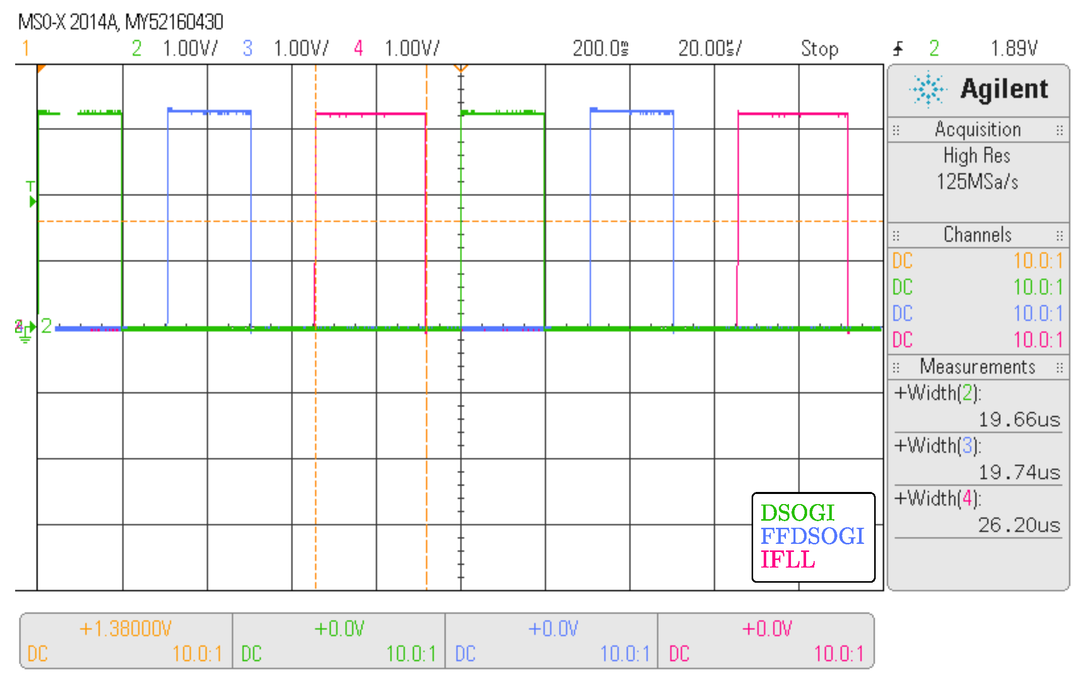
The last test is related to the MCU processing times and it is shown in
Figure 23. In the figure, it is shown the execution times of each method, i.e., the pulse width of each square wave represents the execution time of the algorithm, including the ADCs acquisition time.
7. Conclusions
In the paper, different DSOGI PLL implementations for grid synchronization in weak grids were analyzed. Based on the obtained simulation and experimental results it is possible to conclude that all the DSOGI-based PLL allow to track the three-phase voltage amplitude, frequency, and phase, but show different dynamic and steady-state responses. Based on such results, a benchmark table is presented.
The benchmark table aims to ease the DSOGI-based PLL selection, considering the performance of each implementation for different grid conditions, or events such as low-order harmonics, unbalanced phases, voltage sags, and frequency or phase-step changes. Through the selection of expected individual expected disturbances, it was possible to identify particular scenarios that would result in the choice of each method. The DSOGI is suitable for connection with strong grids, the IFLL in applications where it is required a fast-tracking of the grid frequency during voltage sags or phase jumps, and the FFDSOGI is the most suitable when the phase and/or frequency estimation is required and any of the disturbances can be expected, as far as the grid frequency variations are within the interval of .
Criteria based on expected weak-grid disturbances were applied, resulting in the choice of a suitable DSOGI implementation. Therefore, the FFDSOGI-PLL is adopted as the most performant, according to the requirements within the scope of a weak grid.


