Abstract
This paper describes the recent attempts to apply the zonal model of thermal radiation in numerical simulations of pulverized coal-fired furnaces. Three methods are described: temporary correction of the total exchange areas (TCTEA), repeated run of the numerical simulation (RRNS), and current correction of the total exchange areas (CCTEA). The TCTEA and RRNS methods are based on successive runs of the numerical simulation. The CCTEA method is proof that the zonal model can be used in numerical simulations by the correction of the total exchange areas on the basis of current and initialized surface zone emissivity.
1. Introduction
The process inside pulverized coal-fired furnaces of utility scale boilers is known as a two-phase (gas—particle) turbulent process with chemical reactions and radiative heat exchange. Numerical simulations of such processes are often applied to find the rates of formation and destruction of polluting species (NOx, SOx) [1,2,3] and heat transfer between the flame and surrounding walls [4,5,6]. Numerical simulations provide detailed insights into the processes inside the furnace through the values of physical quantities like velocities, temperatures, combustion, species concentrations, heat flux over the waterwalls, and so on.
Numerical simulations are based on the solution of partial differential equations, which describe processes in the furnace. In the k-ε turbulence model, a time-averaged transport equation of physical quantities is used with the Boussinesq formulation of the relation between Reynolds stresses and mean rates of deformation [7]. A closed form-solution is not possible, and the only possible way is a numerical solution through the iterative procedure of calculation. As the equations are of an elliptic type, every variable is assigned an initial value (at every control volume) at the beginning of the calculation. The variables of the gas phase are solved in the Eulerian frame of reference, while the solid particle phase is solved in the Lagrangian frame of reference.
The numerical solution begins with the adoption of the numerical grid, i.e. the division of the furnace volume into a great number of control volumes and of the furnace walls into surface zones, where the surface zone is actually a boundary surface between the control volume adjacent to the wall and the wall itself. The values of the physical quantities are calculated for the nodes of the control volumes. Differential equations are discretized and linearized, and are solved as a set of linear equations. In this way, the physical quantities of the gas phase (velocity, temperature, species concentration, particle concentration, radiative intensity or flux, turbulent kinetic energy, and decay of the turbulent kinetic energy) are solved. The latter two are the physical quantities of the k-ε turbulent model, and they are determined only if that turbulent model is used.
Solid particles are solved in the Lagrangian frame of reference. Particle velocities, temperatures, and mass are solved along trajectories which represent a group of particles of the same size injected into the furnace at the same location. They are solved by a different method of solution than the gas-phase equations. It is actually a solution of a non-steady condition. The connection between the gas phase and particle phase is conducted by different methods, the most popular of which is the PSI CELL method [8], according to which the solid particles serve as source terms in the corresponding gas-phase equations.
The role of the radiation model in numerical simulations is to provide the radiative source in the enthalpy equation of the gas phase. It also provides a wall flux, which is actually a wall variable but also an important input for the gas-phase equation. Radiation intensity, as the basic physical quantity of radiation heat transfer, depends on the five independent variables: three variables for the location and two angles that represent the direction. In one point, there is an infinite number of radiation intensities, as the number of directions is infinite. The change in radiation intensity along the selected direction is described by the radiation transfer equation (RTE) [9,10]. In numerical simulations, the radiative heat exchange is solved by flux or zonal models. In flux models, the radiative intensity, flux, or a similar quantity is calculated. The most common radiative models are the discrete ordinates model (DOM), the spherical harmonics model (or P1 as the most popular and simplest of these models), the discrete transfer model (DTM), and the six-flux model [7,11,12]. In the DOM, angular discretization is used, and for every division of the whole solid angle (4π sr), the variable (the intensity in that direction) is formed. That variable is the radiation intensity inside that part of the solid angle, that is, the radiation intensity in the corresponding direction. The spatial distribution of every intensity is solved by the finite volume method. A version of the DOM is the finite volume method for radiation, in which the integration is conducted over the control volume and over the division of the solid angle. This results in a somewhat different equation from the one in the DOM. In the spherical harmonics model, the angular dependence of the intensity is approximated by a series of spherical harmonics. P1 is obtained by retaining only the first spherical harmonic. The RTE is transformed into one equation which solves the incident radiation: the integral of the radiation intensity over the solid angles. The DTM is actually a ray—tracing model. Every ray is emitted from the bounding wall and tracked to the point where it hits the opposite wall. The intensity is determined along the path from the corresponding recurrence relation. In the six-flux model, the radiation fluxes are solved along the coordinate axes. In the 3-D model, there are six first-order equations of the fluxes, which are combined into three second-order equations. Flux models easily accommodate the changes in physical quantities needed for the solution, such as the surface emissivity and radiation properties of the medium, i.e. the flame, such as the total extinction coefficient (the sum of the absorption and scattering coefficients) and the scattering albedo. Flux models are easily incorporated into numerical simulations.
The zonal models are the Monte Carlo and Hottel zonal model. They solve the radiative heat exchange on the basis of auxiliary physical quantities. The Monte Carlo method is based on tracking the energy bundles, in which the location of emission, direction, absorption, and so on is determined by a random number. The result of the calculation are exchange factors, which are used to find the radiative exchange. The same exchange factors are found in the Hottel zonal model from the balance of radiative energy. The volume of the furnace (or any other enclosure) is divided into volume zones, and the walls are divided into surface zones. The net radiative exchange of every volume (and surface) zone is the difference between the absorbed and emitted energy. Zonal models are considered more accurate than flux models, but the difficulty with their application is that the exchange factors are solved for one set of radiative properties of the walls and flame, which cannot be changed during the iterative calculation of the numerical simulations. The objective of the investigations described in this paper was to find a way to apply zonal models in numerical investigations.
So far, zonal models have been applied to an inhomogeneous medium in the case of black-walled systems [13,14,15,16,17]. The heat exchange was solved by using DEAs. Modest [10] suggested an application of TEAs for a non-scattering medium. The calculation of DEAs was based on the average absorption coefficient between two zones. These methods were developed for predefined radiative properties, which makes them inapplicable in numerical simulations because of the change in radiative properties from one iteration to the next.
Pulverized coal-fired furnaces are enclosures with gray walls. Pulverized coal flames absorb, emit, and scatter radiation. Furnaces are enclosures that contain several thousands of volume and surface zones. In this paper, recent methods of application of zonal models—TCTEA, RRNS, and CCTEA—in numerical simulations of a pulverized coal-fired furnace are described. These methods were developed for investigations when the end radiative properties (wall emissivities, in this case) were not known. TCTEA and RRNS are not much different from the conventional applications of zonal models. They are based on successive runs of the numerical simulation. The third method, CCTEA, was developed to provide the result with a single run of the numerical investigation. In this method, no radiative properties are determined in advance. In the beginning of the numerical simulation, all variables, including the surface emissivities, start from their initialized values. In the following section, all three methods are described. In these applications, the medium is homogeneous, and the only correction is made for the surface emissivities.
2. Zonal Model
For this study, a 210 MW (electrical output) utility boiler was selected. The schematic layout of the boiler is shown in Figure 1. The boiler is a Π-shaped subcritical natural circulation-boiler with a balanced draft scheme. Feedwater is heated in the economizer before entering the steam drum. The steam is superheated in a series of superheaters. The first-stage (convective) superheater is located in the vertical gas path of the boiler. The second-, third-, and fourth-stage superheaters are located at the top of the furnace and horizontal gas path. After expansion in a high-pressure turbine, the steam is reheated in a two-staged reheater. The boiler produces 180.56 kg s−1 of primary steam (13.7 MPa, 813.0 K) at nominal-load condition.
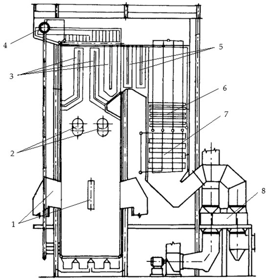
Figure 1.
The layout of the boiler. 1—burner; 2—recirculation opening; 3—radiant steam superheater; 4—steam drum; 5—reheater; 6—convection superheater; 7—economizer; 8—air heater.
The dry-bottom furnace of the boiler is tangentially fired by pulverized coal. The furnace dimensions, the location of the burners, and the location and dimensions of recirculation openings are shown in Figure 2. The furnace is equipped with six burner assemblies (B1–B6), each of which is connected to one fan mill and one recirculation opening (R1–R6). Each burner assembly contains four tiers (one air—dust duct with two ducts of secondary air around it) of the straight-flow burners. The dimensions and arrangement of the burner are shown in Figure 2. Each burner is composed of four stages, each of which contains a coal nozzle and two nozzles for secondary air injection. The pulverized coal—primary air mixture enters the furnace through the coal nozzle at 438.0 K. Secondary air is heated up to 543.0 K. At nominal-load operating conditions, five burners are in operation (B6 and R6 are stand-by).
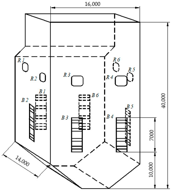
Figure 2.
The model of the furnace used in the numerical simulations.
The furnace is fired by Kolubara lignite. The coal consumption is 73.61 kg s−1. The proximate analysis (as received, wt %) results are as follows: moisture 52.67%, ash 11.23%, volatile 21.46%, fixed carbon 14.64%, lower heating value, as received: 7816.0 kJ kg−1. The ultimate analysis (as received, wt %) results are as follows: carbon 22.70%, hydrogen 2.13%, oxygen 10.39%, nitrogen 0.50%, sulfur 0.39%. The moisture content of the coal during the process in the coal mill is reduced to 14.0% [18]. The particle size distribution of the pulverized coal is given by four fractions (weight percentages): 45.0%, 0–90 μm; 31.0%, 90–200 μm; 22.0%, 200–1000 μm; and 2.0%, particles bigger than 1000 μm. The particle size fractions were formed on the basis of the sieving analysis.
The shape and dimensions of the furnace were slightly modified for application in the numerical simulations. The radiant superheaters were removed from the upper part of the furnace, and the outlet of the furnace was made vertical instead of horizontal. Those modifications were made for reasons of the convergence of the calculation procedure. For the furnace itself, it means that the results obtained for the contraction (above the recirculation openings) are reliable.
The zonal model (or the Hottel zonal model) starts with the division of the furnace volume into volume zones and of the furnace walls into surface zones [19]. For every pair of zones, the direct exchange areas, which represent the heat exchange between the zones in the black-walled system, are found. For a furnace with a great number of zones, the Yamauti principle is used to find the DEAs for all pairs of zones. The Yamauti principle, which states that the DEA of all pairs of zones in the same geometrical relation is the same, can only be used for the homogeneous radiative properties of the medium inside the furnace. DEAs are kept in the matrices and three types of matrices are used: gg, of order M M; sg, of order N M; and ss, of order N N. M is the total number of the volume zones and N is the total number of surface zones. Matrix gg contains all pairs of the volume—volume DEAs, matrix sg contains all pairs of the surface—volume DEAs, and matrix ss contains all pairs of the surface—surface DEAs:
The summation principle for DEAs states that for every surface and volume zone:
The DEAs of the close zones can be calculated in several ways: using the correlations given by Rhine and Tucker [20], using the values given by Siddal [21], or by the numerical method. The DEAs of the distant zones can be calculated using only the distance between their centers. Corrections of DEAs are possible, so that the summation principle can be satisfied within a small defined error.
For the real system enclosure, where surface zones are not black but gray, the total exchange areas (TEAs) must be used. In the method of the original emitters of radiation [19], all zones are cold (their temperature is 0.0 K), except one zone (the original emitter), whose temperature is such that its black emissive power Eb = σT4 = 1.0 W m−2. The balance of radiative energy is formed, and a system of linear equations is obtained in the form a = Bc, where a is the known column matrix of order (M + N) 1, c is the unknown column matrix of order (M + N) 1, and B is the square matrix of coefficients of order (M + N) (M + N). All elements of the known column matrix are zero, except for the zone that is not cold. In total, there are M + N known column matrices a. The elements of vector c, obtained as a solution of the equation, are used to find the TEAs. That equation is solved by the method of decomposition to lower and upper triangular matrices (LU decomposition) with pivoting [22]. TEAs are kept in the matrices:
The summation principle of TEAs states that:
The summation principle provides the exact values of the sum of all TEAs connected with a certain surface or volume zone. It enables corrections of the TEAs (calculated by any method) in order to provide zero radiative heat exchange in the isothermal system within a small defined error.
TEAs are found for the homogeneous radiative properties of the medium, defined for each volume zone. The emissivities of the surface zones do not have to have the same values; they just have to be defined. In the conventional application of the zonal model, all results are obtained for the unchanged radiative properties of the flame and furnace walls. In that or a similar way, the zonal model was used in numerical simulations of pulverized coal-fired and other furnaces [23,24,25,26,27,28,29,30,31]. The radiative property of the gas-phase (absorption coefficient) could be determined by the simple gray gas model or by the weighted sum of the gray gases model. The scattering of radiation is a consequence of the presence of fly ash particles.
The TCTEA method is based on the successive run of the numerical simulation [32]. In the first run, all variables start from the initial values, and the radiative properties of the flame and furnace walls are also homogeneous. At the end of the numerical simulation, the values of all variables are written into the files. The emissivities of the surface zones are written into the files and a new set of TEAs is determined. In the next run of the numerical simulation, all variables start from the values obtained at the end of the previous simulation. Again, at the end of the numerical simulation, the emissivities of the surface zones are written into the files, and a new set of TEAs is found for the use in the next numerical simulation.
The RRNS method is similar to the TCTEA method, with the difference that the variables in every simulation start from the initial values, except for the surface emissivities [32]. At the end of the numerical simulation, the emissivities of the surface zones are written into the files, and a new set of TEAs is found for the next numerical simulation. Several simulations (three or four) are needed to reach the convergent solution.
In the CCTEA method [33], the results are obtained after one run of the numerical simulation. Corrections of the surface emissivities are made on the basis of the surface zone temperature and the dependence of the surface emissivities on temperature. Corrections of the TEAs are made after every iteration, in accordance with the new values of the surface emissivities and summation principle. In the ith iteration, the surface emissivity of all surface zones is different from the initial values. When the surface zone si is analyzed, the elements of the SS matrix in the ith row are changed according to the emissivities of the surface zones. Then, the ith row of the SG matrix is modified in order to satisfy the new sum of surface zone si. Simultaneously, the new sums of the columns of the SG matrix are obtained. Finally, the elements of the GG matrix are modified to satisfy the sum of the volume zones. For the corrected values of the TEAs, the new radiative source terms and net wall fluxes needed for the current iteration are found.
3. Mathematical Model
The numerical simulation in these investigations is based on the solution of the mathematical model of the RANS type. The process inside the furnace is a two-phase turbulent (gas—particle) reacting flow with radiative heat exchange. The model based on the time-averaged physical quantities of the gas phase was used [34]. The numerical simulation contains three algorithms: the first one for the solution of the gas-phase equations, the second one for the solution of the dispersed phase, and the third one for the solution of the radiative heat exchange. The numerical simulation is based on in-house developed software.
The gas phase is described by the time-averaged differential equations in the Eulerian reference frame:
where ρ (kg m−3) is the gas-phase density, U (m s−1) is the velocity vector, Φ is the general gas-phase variable, ΓΦ (kg m−1 s−1) is the turbulent diffusivity, SΦ (W m−3) is the source term, and SΦ,p (W m−3) is the source term due to particles. Equation (1) was used for the solution of the gas-phase velocities, temperature, component concentrations, turbulent kinetic energy, the rate of turbulent kinetic energy dissipation, and number concentration of particles. The gas-phase density was determined from the equation of state. The system of equations was closed by the k-ε model of turbulence. The pressure field was solved by the SIMPLE algorithm, which combines the momentum and continuity equations to find the pressure corrections. A staggered grid was used to find the velocity and pressure field.
The enthalpy equation from which the flame temperature is solved is:
where cf (J kg−1 K−1) is the specific heat of the flame, ΓH (kg m−1 s−1) is the turbulent diffusivity for enthalpy, P (N m−2) is the pressure, SH,com (W m−3) is the source term due to combustion, and (W m−3) is the radiative source term. The enthalpy equation is solved for the thermal equilibrium between the gas and dispersed phases [34].
The objective of the radiation model in the numerical simulation is to find the radiative source term of the control volumes and wall fluxes of the surface zones. The radiative source term is the difference between the absorbed and lost radiation energy:
where (m2) is the volume—volume total exchange area, (m2) is the surface—volume total exchange area, M is the total number of the volume zones, N is the total number of the surface zones, V (m3) is the volume, Kt (m−1) is the total extinction coefficient, and ω (-) is the scattering albedo. The total extinction coefficient Kt = Ks + Ka, where Ks (m−1) is the scattering coefficient and Ka (m−1) is the absorption coefficient. The term represent the absorption coefficient of the medium, since . (In the case of a pulverized coal flame, the absorption coefficient of the flame is the sum of the absorption coefficients of the gas phase and the dispersed phase. The scattering coefficient of the flame is that of the dispersed phase. The total extinction coefficient of the flame is the sum of all radiative coefficients).
The wall flux of the surface zone si is also the difference between the absorbed and lost radiation energy:
where (m2) is the surface—surface total exchange area, ϵw (-) is the wall emissivity, A (m2) is the surface area, and (W) is the heat transfer rate. The total exchanged heat Qtot (W) was obtained by summing all the heat transfer rates for the surface zones that are the solid walls: .
The heat transfer rates through the furnace waterwalls were determined for a two-layer wall composed of a 4.0 mm thick metal wall and an ash deposit layer, whose thickness was adopted. Along one side of the two-layer wall, there is a flow of a two-phase steam of boiling water, and there is hot furnace medium along the other side. The water—steam mixture temperature is determined in accordance with the boiling pressure, Tb = 615.0 K. For the given wall flux, the temperature of the inner surface of the metal wall is determined using the convective heat transfer between the metal wall and the water—steam mixture, whereas the temperatures of the outer surface of the metal wall are determined using the one-dimensional steady-state heat conduction equation. The thermal conductivity of the metal wall can be found in [35,36].
The wall temperature is determined using the formula for one-dimensional steady-state heat conduction:
where h (W m−2 K−1) is the convection heat transfer coefficient, Km (W m−1 K−1) is the thermal conductivity of the metal wall, lm (mm) is the thickness of the metal wall, Kef (W m−1 K−1) is the effective thermal conductivity of the deposit layer, and ld (mm) is the thickness of the deposit layer.
The functional dependence of effective thermal conductivity and surface emissivity on temperature must be continuous for this investigation. The dependence of the effective thermal conductivity was adopted from the work of Boow and Goard [37] for a coal ash sample whose silica ratio was 62. It is an increasing function of temperature. At a low temperature range, from 673.0 to 1173.0 K, the effective thermal conductivity increases very slowly with temperature. At 873.0 K, its value is approximately 0.20 W m−1 K−1. At a medium temperature interval, from 1173.0 to 1373.0 K, sintering occurs, and the increase in effective thermal conductivity with temperature becomes steeper. At a high temperature interval, above 1373.0 K, fusion begins, and the dependence of the effective thermal conductivity on temperature becomes steeper than at the medium temperature interval. At 1573.0 K, every sample is completely fused, and the effective thermal conductivity of every sample is higher than 1.88 W m−1 K−1. Upon cooling, the effective thermal conductivity is greater than that during the heating for the same temperature, as the physical structure of the sample is changed. The dependence of the effective thermal conductivity on temperature was determined in the polynomial form:
The values of the coefficients aj can be found in [38]. The dependence of surface emissivity on temperature was also adopted for the same sample of coal ash. The dependence of surface emissivity on temperature was at a minimum. The surface emissivity is 0.85 at 560.0 K. Upon heating, it decreases to 0.58 at 1300.0 K and increases with further heating. At 1400.0 K, the surface emissivity is 0.7.
The dispersed phase is described by differential equations of motion and change in mass and energy in the Lagrangian reference frame. The motion of the particles is tracked along trajectories with a constant number of particles. Particle velocity is the sum of the convective and diffusion components. Convective velocity is obtained by tracking the particles along the trajectories, while the diffusion component is obtained from the particle number concentration. The phases are connected by the PSI CELL method, in which the presence of particles is taken into account by additional sources in the transport equations of the gas phase. The influences of the particles on turbulent kinetic energy and its rate of dissipation (i.e. turbulent modulation) are also taken into account through additional source terms in the gas-phase equations. Particle collisions are neglected, while particle-to-wall collisions are considered with a certain degree of elasticity. More details about the modeling of the dispersed phase can be found in [39].
Heterogeneous reactions of coal combustion are modeled in the kinetic diffusion regime. The change in particle mass with time is described by the following formula:
where (kg) is the mass of the particle, t (s) is time, (m2) is the particle surface area, (kg mol−1) is the particle molar mass, (kmol m−3) is the oxidant molar concentration, (m s−1) is the reaction rate in the kinetic regime, and (m s−1) is the oxidizer mass transfer diffusion parameter. In the kinetic diffusion regime, the reaction rates and are approximately equal. Details of the combustion model can be found in [40].
Boundary conditions at the inlet are defined by the nature of the problem and those at the outlet by the continuity condition. Conditions near the wall are described by wall functions. The wall temperature, determined by Equation (5), is not constant.
The thermophysical properties of the gas phase were determined from the equation of state, tabulated values, and empirical relations. Discretization of the gas-phase equations was achieved by the finite volume method (a version of the finite difference method) and a hybrid differencing scheme. The stability of the iterative procedure was provided by the under-relaxation method [7]. Using this method, the value of the variable determined in the ith iteration is partly the value of the ith and previous iteration.
4. Results and Discussion
Radiative heat exchange was solved on a coarse numerical grid composed of cubical volume zones with an edge dimension of 1.0 m. The furnace volume was divided into 7956 volume zones and the furnace walls were divided into 2712 surface zones. Flow field was solved on a fine numerical grid which was obtained by dividing every volume zone into 64 control volumes. The total number of control volumes (the numerical grid used for calculation of the fluid flow) was 620,136. The agreement with the experimental data and a grid independence study are shown in [34]. The direct exchange areas of the close zones were determined using correlations [20]. Total exchange areas were calculated by the method of original emitters of radiation [19]. Improvements in the values of total exchange areas were accomplished using generalized Lawson’s smoothing method [14].
Heat flux , wall temperature , and wall emissivity were determined for the resolution of the surface zones. The only gas-phase variable used in this comparison was flame temperature , determined for the resolution of control volumes. The absolute relative difference (ARD) values of the selected variables were determined by formula (14):
where η designates the selected variable. The ARDs were determined using the difference between the results obtained by the CCTEA and RRNS methods, as it was determined that the differences between the RRNS and TCTEA methods were small, and the RRNS method was selected as it was easier to apply [32]. The differences in the results were found using the mean absolute relative difference (MARD):
where n is the population size. For the wall variables, the population size is the total number of the surface zones that represent the solid wall. (The wall that represents the furnace bottom was also excluded from the analysis.) For the flame temperature, the population size is the total number of control volumes for which the variable value is determined.
The MARD values for the initial values of surface emissivity, total extinction coefficient, and ash deposit layer thicknesses are shown in Figure 3a–c. In all diagrams, the MARD is the smallest for surface emissivity, then wall temperature, flame temperature, and wall fluxes. The highest MARD slightly exceeds 2.0%. The MARD was approximately constant for the various initial surface emissivities and total extinction coefficients. With the increase in deposit thickness, the MARD decreases for wall flux and flame temperature and increases for wall temperature and wall emissivity.
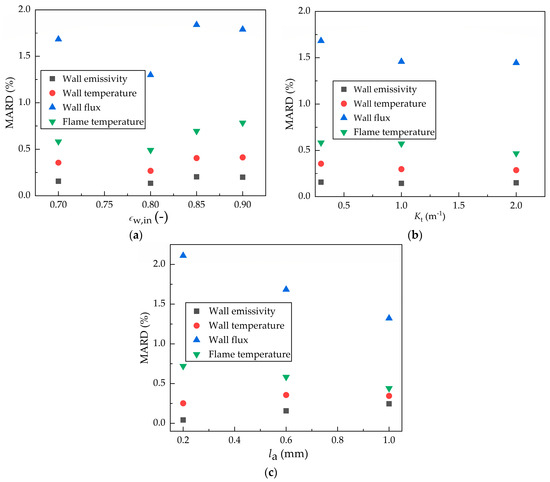
Figure 3.
MARD: (a) Kt = 0.3 m−1, la = 0.6 mm; (b) = 0.70, la = 0.6 mm; (c) Kt = 0.3 m−1, = 0.70.
The values of the wall flux obtained by the CCTEA method and its ARDs are shown in Figure 4a,b for the front wall. The biggest values of wall fluxes were obtained in the area close to the burners, according to the expectations. The ARD values are the highest in the area where the wall fluxes are the lowest. In addition, some of the ARDs are positive and some are negative, so that the differences in the mean wall flux are smaller than the MARD for the wall flux. For example, for Kt = 0.3 m−1, = 0.70, and la = 0.6 mm, the difference in the mean wall flux is 0.83%, which is approximately half of the values obtained for the MARD.
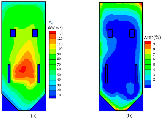
Figure 4.
Wall flux, front wall, Kt = 0.3 m−1, = 0.70, la = 0.6 mm: (a) values of wall flux; (b) ARD.
The wall temperature values of the front wall and the corresponding ARDs are shown in Figure 5a,b. The wall temperature is the highest in the area where the wall flux is the highest, according to Equation (11). Similarly to the wall fluxes, the ARDs are highest in the parts where the wall temperatures are the lowest.
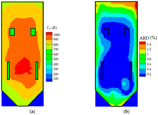
Figure 5.
Wall temperature, front wall, Kt = 0.3 m−1, = 0.70, la = 0.6 mm: (a) values of the wall temperature; (b) ARD.
The wall emissivity and the corresponding ARDs for the same wall are shown in Figure 6a,b. The wall emissivities are the lowest in the areas where the wall fluxes are the highest, according to the dependence of emissivity on temperature. The values of the ARDs are lower than those for wall fluxes and temperatures, in accordance with the smallest values of the MARD, shown in Figure 3.
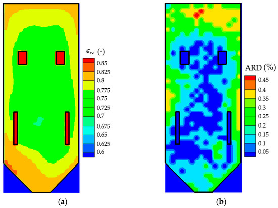
Figure 6.
Wall emissivity, front wall, Kt = 0.3 m−1, = 0.70, la = 0.6 mm: (a) values of the wall emissivity; (b) ARD.
The flame temperature and its ARDs are shown in Figure 7a,b. The flame temperature is the highest near the burners, because of the rapid heat release from combustion. In the other parts of the furnace, the flame temperature decreases because of the radiative heat exchange with the furnace walls. The values of the ARDs are also lowest in the parts of the furnace where the temperature levels are not the highest.
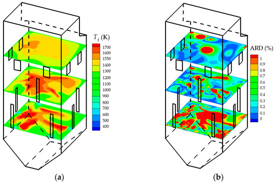
Figure 7.
Furnace temperature, Kt = 0.3 m−1, = 0.70, la = 0.6 mm: (a) values of the furnace temperature; (b) ARD.
The obtained results show that the CCTEA method provides acceptable results of the numerical simulations. The CCTEA method was derived for application in the numerical simulations. As it can be seen from the figures, there are no sudden and abrupt changes in the surface emissivities. This version of the method is based on the change in the surface emissivity of the ash deposits. The accuracy of the method certainly depends on the interval of the values of surface emissivities.
The CCTEA method is simple and no new terms other than those defined by the zonal model are needed. A problem of the CCTEA method could be the negative values of the TEAs, which could happen because of the method of calculation. No negative values of the TEAs were recorded. So far, the method has been derived for the homogeneous radiative properties of the flame. The application of the method for non-homogeneous radiative properties of the flame will be solved in the following investigations on the method. Also, confirmation of the method in comparison with other radiation models should be conducted.
5. Conclusions
Three methods for the application of the zonal model of radiative heat exchange in numerical simulations of pulverized coal-fired furnaces were described. The methods allowed for the corrections of surface zone emissivities. At the end of the numerical simulation, new values of surface zone emissivities were determined, stored in the files, and used for the calculation of a new set of TEAs. In the TCTEA method, all variables (including surface emissivities) start from the values obtained by the previous numerical simulation. In the RRNS method, all variables start from the initial values except for the surface emissivities. Both methods provide similar results, and the RRNS method was adopted for further work as its application is easier. For both methods, the numerical simulation should be run three or four times to reach the convergent solution.
The CCTEA method provides the results by a single run of the numerical simulation. The method is based on the correction of surface emissivity during the calculation and on the correction of TEAs based on the summation principle. A comparison of the results showed a small difference in the results obtained by the CCTEA and RRNS methods. The next task would be to develop the CCTEA method to include the non-homogeneous radiative properties of the flame.
Funding
The research was funded by the Ministry of Science, Technological Development and Innovation of the Republic of Serbia (Contract Annex: 451-03-136/2025-03/200017).
Institutional Review Board Statement
Not applicable.
Informed Consent Statement
Not applicable.
Data Availability Statement
Data is contained within the article.
Conflicts of Interest
The author declare no conflict of interest.
References
- Belošević, S.; Tomanović, I.D.; Crnomarković, N.Đ.; Milićević, A.; Tucaković, D.R. Numerical study of pulverized coal-fired utility boiler over a wide range of operating conditions for in-furnace SO2/NOx reduction. Appl. Therm. Eng. 2016, 94, 657–669. [Google Scholar] [CrossRef]
- Askarova, A.; Georgiev, A.; Bolegenova, S.; Beketayeva, M.; Maximov, V.; Bolegenova, S. Computational modeling of pollutants in furnaces of pulverized coal boilers of the republic of Kazakhstan. Energy 2022, 258, 124826. [Google Scholar] [CrossRef]
- Tomanović, I.; Belošević, S.; Crnomarković, N.; Milićević, A.; Tucaković, D. Numerical modeling of in-furnace sulfur removal by sorbent injection during pulverized lignite combustion. Int. J. Heat Mass Transf. 2019, 128, 98–114. [Google Scholar] [CrossRef]
- Chudnovsky, B.; Talanker, A. Effect of bituminous coal properties on heat transfer characteristic in the boiler furnaces. In Proceedings of the IMECE2004, 2004 ASME International Mechanical Engineering Conference, Anaheim, CA, USA, 13–19 November 2004. [Google Scholar] [CrossRef]
- Ma, Z.; Iman, F.; Lu, P.; Sears, R.; Kong, L.; Rokanuzzaman, A.S.; McCollor, D.P.; Benson, S.A. A comprehensive slagging and fouling prediction tool for coal-fired boilers and its validation/application. Fuel Process. Technol. 2007, 88, 1035–1043. [Google Scholar] [CrossRef]
- Modlinski, N.J. Computational modelling of a tangentially fired boiler with deposit formation phenomena. Chem. and Process Eng. 2014, 35, 361–368. [Google Scholar] [CrossRef]
- Versteeg, H.K.; Malalasekera, W. An Introduction to Computational Fluid Dynamics, 2nd ed.; Pearson Education: Harlow, UK, 2007; pp. 417–444. [Google Scholar]
- Crowe, C.T.; Sharma, M.P.; Stock, D.E. The particle-source-in cell (PSI-CELL) model for gas-droplet flows. J. Fluids Eng. 1977, 99, 325–332. [Google Scholar] [CrossRef]
- Howell, J.R.; Siegel, R.; Menguc, M.P. Thermal Radiation Heat Transfer, 5th ed.; CRC Press: Boca Raton, FL, USA, 2010; pp. 493–534. [Google Scholar]
- Modest, M.F. Radiative Heat Transfer, 3rd ed.; Academic Press: New York, NY, USA, 2013; pp. 279–302. [Google Scholar]
- Viskanta, R. Radiative Transfer in Combustion Systems; Begell House: New York, NY, USA, 2005; pp. 251–283. [Google Scholar]
- Oran, E.S.; Boris, J.P. Numerical Simulation of Reactive Flow; Cambridge University Press: New York, NY, USA, 2001; pp. 488–519. [Google Scholar]
- Pieri, G.; Sarofim, A.F.; Hottel, H.C. Radiant heat transfer in enclosures: Extension of Hottel-Cohen zone method to allow for concentration gradients. J. Inst. Fuel 1973, 46, 321–330. [Google Scholar]
- Mechi, R.; Farhat, H.; Guedri, K.; Halouani, K.; Said, R. Extension of the zonal method to inhomogeneous non-grey semi-transparent medium. Energy 2010, 35, 1–15. [Google Scholar] [CrossRef]
- Bordbar, M.H.; Hyppanen, T. The correlation based zonal method and its application to the back pass channel of oxy/air-fired CFB boiler. Appl. Therm. Eng. 2015, 78, 351–363. [Google Scholar] [CrossRef]
- Yuen, W.W.; Takara, E.E. The zonal method: A practical solution method for radiative transfer in nonisothermal inhomogeneous media. Annu. Rev. Heat Transf. 1997, 8, 153–215. [Google Scholar] [CrossRef]
- Yuen, W.W. The multiple absorption coefficient zonal method (MACZM), an efficient computational approach for the analysis of radiative heat transfer in multidimensional inhomogeneous nongray media. Numer. Heat Transf. Part B 2006, 49, 89–103. [Google Scholar] [CrossRef][Green Version]
- Pavlovic, P.; Riznic, J. Results of Thermal Measurements in Furnace of Nikola Tesla Power Plant Boiler No. 2; Report No.: IBK-LTFT-104; Institute of Nuclear Sciences Boris Kidric: Belgrade, Yugoslavia, 1977; pp. 3–4. [Google Scholar]
- Hottel, H.C.; Sarofim, A.F. Radiative Transfer; McGraw-Hill: New York, NY, USA, 1967; pp. 408–437. [Google Scholar]
- Rhine, J.M.; Tucker, R.J. Modeling of Gas-Fired Furnaces and Boilers; McGraw-Hill: New York, NY, USA, 1991; pp. 411–424. [Google Scholar]
- Siddal, R.G. Accurate evaluation of radiative direct-exchange areas for rectangular geometries. In Proceedings of the Eight International Heat Transfer Conference, San Francisco, CA, USA, 17–22 July 1986. [Google Scholar]
- Press, W.H.; Flannery, B.P.; Teukolsky, S.A.; Vetterling, W.T. Numerical Recipes, The Art of Scientific Computing; Cambridge University Press: New York, NY, USA, 1986; pp. 19–76. [Google Scholar]
- Niu, Z.; Wong, K.F.V. Adaptive simulation of boiler unit performance. Energy Convers. Manag. 1998, 39, 1383–1394. [Google Scholar] [CrossRef]
- Marakis, J.G.; Papapavlou, C.H.; Kakaras, E. A parametric study of radiative heat transfer in pulverised coal furnaces. Int. J. Heat Mass Transf. 2000, 43, 2961–2971. [Google Scholar] [CrossRef]
- Batu, A.; Selcuk, N. Modeling of radiative heat transfer in the freeboard of a fluidized bed combustor using the zone method of analysis. Turk. J. Eng. Environ. Sci. 2002, 26, 49–58. [Google Scholar]
- Chudnovsky, B.; Talanker, A.; Kogan, B.; Daniliuc, M.; Lev, S.; Frega, L. Combination of Advanced Supervision System FURNACE With Continues Visual Monitoring ORFEUS for Proper On-Line Performance Analysis of the Furnace Firing Coal in Large Utility Boilers. In Proceedings of the ASME Power Conference, Albuquerque, NM, USA, 21–23 July 2009. [Google Scholar] [CrossRef]
- Mechi, R.; Radhouani, M.S.; Farhat, H.; Halouani, K. Radiative transfer modeling in an incinerator of polluting wood pyrolysis emissions. Int. J. Therm. Sci. 2004, 43, 697–708. [Google Scholar] [CrossRef]
- Bordbar, M.H.; Hyppänen, T. Modeling of radiation heat transfer in a boiler furnace. Adv. Stud. in Theor. Phys. 2007, 1, 571–584. [Google Scholar]
- Diez, L.I.; Cortes, C.; Campo, A. Modelling of pulverized coal boilers: Review and validation of on-line simulation techniques. Appl. Therm. Eng. 2005, 25, 1516–1533. [Google Scholar] [CrossRef]
- Silva, C.V.; Franca, F.H.R.; Vielmo, H.A. Analysis of the turbulent, non-premixed combustion of natural gas in a cylindrical chamber with and without thermal radiation. Combust. Sci. Technol. 2007, 179, 1605–1630. [Google Scholar] [CrossRef]
- Tan, C.-K.; Jenkins, J.; Ward, J.; Broughton, J.; Heeley, A. Zone modelling of the thermal performances of a large-scale bloom reheating furnace. Appl. Therm. Eng. 2013, 50, 1111–1118. [Google Scholar] [CrossRef]
- Crnomarkovic, N.; Belosevic, S.; Tomanovic, I.; Milicevic, A. Determination of the wall variables within the zonal model of radiation inside a pulverized coal-fired furnace. Facta Univ. Ser. Mech. Eng. 2018, 16, 219–232. [Google Scholar] [CrossRef]
- Crnomarković, N.; Belošević, S.; Tomanović, I.; Milićević, A. New application method of the zonal model for simulations of pulverized coal-fired furnaces based on correction of total exchange areas. Int. J. Heat Mass Transf. 2020, 149, 119192. [Google Scholar] [CrossRef]
- Crnomarkovic, N.; Sijercic, M.; Belosevic, S.; Tucakovic, D.; Zivanovic, T. Radiative heat exchange inside the pulverized lignite fired furnace for the gray radiative properties with thermal equilibrium between phases. Int. J. Therm. Sci. 2014, 85, 21–28. [Google Scholar] [CrossRef]
- Singer, J.G. Combustion Fossil Power; Combustion Engineering: Stamford, CT, USA, 1991; pp. 17.1–17.32. [Google Scholar]
- Kaye, G.W.C.; Laby, T.H. Tables of Physical and Chemical Constants; Longman: New York, NY, USA, 1986; pp. 44–70. [Google Scholar]
- Boow, J.; Goard, P.R.C. Fireside deposits and their effect on heat transfer in a pulverized coal fired boiler, part 3-The influence of the physical characteristics of the deposit on its radiant emittance and effective thermal conductance. J. Inst. Fuel 1969, 42, 412–419. [Google Scholar]
- Crnomarkovic, N.D.; Sijercic, M.A.; Belosevic, S.V.; Tucakovic, D.R.; Zivanovic, T.V.; Tomanovic, I.D.; Stojanovic, A.D. Numerical determination of the impact of the ash deposit on the furnace walls to the radiative heat exchange inside the pulverized coal fired furnace. In Proceedings of the International Conference Power Plants 2014, Zlatibor, Serbia, 28–31 October 2014. [Google Scholar]
- Belošević, S.; Tomanović, I.; Crnomarković, N.; Milićević, A. Full-scale CFD investigation of gas-particle flow, interactions and combustion in tangentially fired pulverized coal furnace. Energy 2019, 179, 1036–1053. [Google Scholar] [CrossRef]
- Belosevic, S.; Sijercic, M.; Crnomarkovic, N.; Stankovic, B.; Tucakovic, D. Numerical prediction of pulverized coal flame in utility boiler furnaces. Energy Fuels 2009, 23, 5401–5412. [Google Scholar] [CrossRef]


Disclaimer/Publisher’s Note: The statements, opinions and data contained in all publications are solely those of the individual author(s) and contributor(s) and not of MDPI and/or the editor(s). MDPI and/or the editor(s) disclaim responsibility for any injury to people or property resulting from any ideas, methods, instructions or products referred to in the content. |
© 2025 by the author. Licensee MDPI, Basel, Switzerland. This article is an open access article distributed under the terms and conditions of the Creative Commons Attribution (CC BY) license (https://creativecommons.org/licenses/by/4.0/).