Multi-Objective MILP Models for Optimizing Makespan and Energy Consumption in Additive Manufacturing Systems ^†

Abstract

Additive manufacturing (AM) is revolutionizing industrial production by enabling the fabrication of complex, customized components with reduced material waste. However, the scheduling of AM machines presents significant challenges in terms of optimizing both time-related performance and energy consumption. This paper introduces a novel multi-objective mixed-integer linear programming (MILP) model for scheduling AM machines with the dual objectives of minimizing makespan and energy consumption. We address the single-machine environment with detailed mathematical formulation that accounts for machine-specific parameters such as power consumption rates during different operational states, including printing, setup, and idle modes. Additionally, we consider part-specific characteristics including height, area requirements, and volume, ensuring practical feasibility constraints are met. The proposed model is validated using a comprehensive set of test problems, with optimal solutions reported for small to medium-sized instances. For larger problem instances, where computational complexity prevents finding optimal solutions within reasonable time limits, we report the best solutions obtained under specified time constraints. Computational experiments demonstrate that our approach effectively balances the trade-off between makespan and energy consumption, providing valuable insights for production planning in AM facilities. The results indicate potential energy savings of up to 18% compared to makespan-only optimization approaches, with minimal impact on overall completion times.

1. Introduction

Additive manufacturing (AM), commonly known as 3D printing, has emerged as a transformative technology in modern manufacturing systems. Indeed, AM is frequently cited as a key enabler of Industry 4.0 and facilitates rapid prototyping and distributed manufacturing [1]. Unlike traditional subtractive methods, AM builds parts layer by layer from 3D model data, offering unprecedented design flexibility, resource efficiency, and the ability to produce complex geometries that would be impossible or prohibitively expensive with conventional techniques [2]. The ability to create highly customized products directly from digital models is a significant driver of its adoption in fields like medical implants and consumer goods [3]. Furthermore, the layer-wise approach fundamentally redefines design rules compared to conventional manufacturing, opening up new possibilities for functional integration and topology optimization [4]. The adoption of AM has expanded rapidly across various industries, including aerospace, automotive, healthcare, and defense, with the global AM market projected to reach $12 billion by 2025 [5].

The unique capabilities of AM have enabled significant advancements in these sectors. For instance, NASA has utilized additively manufactured parts for Mars Rover test vehicles, while General Electric has applied the technology to directly manufacture fuel nozzles that previously required the assembly of 20 different components [6]. Perhaps most notably, AM technology now allows astronauts to fabricate parts and tools in space on demand, dramatically reducing the logistical challenges associated with space missions.

Despite these advantages, AM facilities face substantial operational challenges. The high acquisition cost of AM machines, coupled with the time-intensive nature of the layer-by-layer production process, necessitates efficient scheduling to maximize utilization and minimize operating costs. Effectively scheduling AM machines involves complex decisions regarding part orientation, nesting within the build volume, and batch formation, often formulated as NP-hard combinatorial optimization problems [7]. Optimizing build layouts and sequences is crucial not only for throughput but also for ensuring part quality and resource efficiency [8]. While the cost structures for AM facilities have been extensively studied in the literature [9], research on optimizing time and energy-related performance measures in AM machine scheduling remains limited.

Building upon the groundbreaking work of Kucukkoc [10], who introduced MILP models to minimize makespan in AM machine scheduling, our research extends this approach by incorporating energy consumption as a critical second objective. This multi-objective perspective is particularly relevant given the increasing emphasis on sustainable manufacturing practices and the significant energy requirements of AM processes. Reducing the environmental footprint of manufacturing processes is a growing global concern, making energy-efficient operations a critical goal for AM adoption [11]. Studies have shown that energy consumption in AM can vary substantially based on machine utilization patterns, part orientations, and batch configurations [12,13]. Researchers have developed models to estimate AM energy consumption, considering factors like material type, process parameters, and machine states (idle, heating, printing) [14]. Investigating the interplay between scheduling decisions and energy usage is essential for developing truly sustainable AM practices [15].

In this paper, we formulate the AM machine scheduling problem with the dual objectives of minimizing makespan and energy consumption. Similar to earlier work, we consider three machine configurations: (1) single machine environment, denoted as $1\left|batch\left\{AM\right\}\right|C_{max},E$; (2) parallel identical machines, denoted as $Pm\left|batch\left\{AM\right\}\right|C_{max},E$; and (3) parallel non-identical machines, denoted as $Rm\left|batch\left\{AM\right\}\right|C_{max},E$. For each configuration, we develop MILP models that account for machine-specific energy consumption parameters during different operational states, including printing, setup, and idle modes.

Our approach differs from traditional batch scheduling problems in several key aspects. First, the processing time of parts in AM is resource-dependent and dynamically determined by the total volume of parts included in a job batch, as well as by the maximum height of those parts. Specifically, the batch processing time in many AM technologies depends on the maximum height of any part within the batch, rather than just the sum of individual processing times which creates unique scheduling challenges [16]. Second, energy consumption varies significantly based on the machine state and the specific characteristics of the parts being produced. Third, there exists a complex trade-off between machine utilization, job completion time, and energy efficiency that must be carefully balanced. The trade-off between minimizing makespan (often achieved by fuller batches) and minimizing energy (which might favor smaller, quicker batches or strategic idling) necessitates multi-objective optimization approaches [17].

The remainder of this paper is organized as follows. Section 2 presents our mathematical models for single-machine scheduling with energy considerations. Section 3 provides a comprehensive computational study of the proposed models across various problem instances, including extensions to parallel identical and non-identical machine environments. Finally, Section 4 concludes the paper with insights and directions for future research.

2. Single-Machine Environment with Energy Considerations ($\mathbf{1}\left|\mathbf{batch}\left\{\mathbf{AM}\right\}\right|{\mathbf{C}}_{\mathbf{max}},\mathbf{E}$)

In this section, we present our mathematical model for scheduling a single AM machine with the dual objectives of minimizing makespan and energy consumption. The problem consists of one AM machine and a set of parts $i\in I=\{1,2,\dots ,i_n\}$ to be allocated to a set of jobs $j\in J=\{1,2,\dots ,j_n\}$, where $j_n\le i_n$.

2.1. Parameters and Variables

2.1.1. Part-Related Parameters

The parts may have different specifications, characterized by the following parameters:

• $h_i$: Height of part i (cm).
• $a_i$: Area required by part i (cm²).
• $v_i$: Volume of part i (cm³).

2.1.2. Machine-Related Parameters

The machine characteristics are defined by the following parameters:

• $VT$: Time spent to form per unit volume of material (hr/cm³).
• $HT$: Time spent for powder-layering per unit height (hr/cm).
• $SET$: Setup time needed for initializing and cleaning (hr).
• $MA$: Production area capacity of the machine’s tray (cm²).
• $P_{print}$: Power consumption during printing operation (kW).
• $P_{layer}$: Power consumption during layer formation (kW).
• $P_{setup}$: Power consumption during setup operations (kW).
• $P_{idle}$: Power consumption during idle time (kW).

2.1.3. Decision Variables

• $X_{ji}\in \{0,1\}$: Binary variable that equals 1 if part i is assigned to job j; 0 otherwise.
• $Z_j\in \{0,1\}$: Binary variable that equals 1 if job j is utilized (i.e., at least one part is assigned to it); 0 otherwise.
• $C_j$: Completion time of job j (hr).
• $C_{max}$: Makespan, i.e., the maximum completion time among all jobs (hr).
• $E_j^{print}$: Energy consumed during printing operations for job j (kWh).
• $E_j^{layer}$: Energy consumed during layer formation for job j (kWh).
• $E_j^{setup}$: Energy consumed during setup operations for job j (kWh).
• $E_{total}$: Total energy consumption (kWh).

2.2. Mathematical Model

2.2.1. Objective Functions

Our model considers two objectives:

$$min{Z}_1=C_{max}=\underset{j\in J}{max}\left\{C_j\right\}$$

(1)

$$min{Z}_2=E_{total}=\sum _{j\in J}(E_j^{print}+E_j^{layer}+E_j^{setup})$$

(2)

We adopt the weighted-sum method to combine these objectives:

$$minZ=\alpha ·{\displaystyle \frac{C_{max}}{C_{max}^{*}}}+(1-\alpha )·{\displaystyle \frac{E_{total}}{E_{total}^{*}}}$$

(3)

where $C_{max}^{*}$ and $E_{total}^{*}$ are the optimal values of makespan and energy consumption when optimized individually, and $\alpha \in [0,1]$ is a weighting factor representing the relative importance of makespan versus energy consumption.

2.2.2. Production Time Calculation

The production time for job j is calculated as follows:

$$P{T}_j=SET·Z_j+VT·\sum _{i\in I}{v}_i·X_{ji}+HT·\underset{i\in I}{max}\{h_i·X_{ji}\}\forall j\in J$$

(4)

2.2.3. Energy Consumption Calculation

The energy consumption components for job j are calculated as follows:

$$E_j^{print}=P_{print}·VT·\sum _{i\in I}{v}_i·X_{ji}\forall j\in J$$

(5)

$$E_j^{layer}=P_{layer}·HT·\underset{i\in I}{max}\{h_i·X_{ji}\}\forall j\in J$$

(6)

$$E_j^{setup}=P_{setup}·SET·Z_j\forall j\in J$$

(7)

2.2.4. Constraints

The following constraints ensure the feasibility of the solution:

• Part Occurrence Constraint

Each part must be assigned to exactly one job:

$$\sum _{j\in J}{X}_{ji}=1\forall i\in I$$

(8)

• Area Capacity Constraint

The total area of parts assigned to a job must not exceed the machine’s capacity:

$$\sum _{i\in I}{a}_i·X_{ji}\le MA\forall j\in J$$

(9)

• Job Utilization Constraint

Jobs are utilized in an incremental order:

$$\sum _{i\in I}{X}_{(j+1)i}\le \psi ·\sum _{i\in I}{X}_{ji}\forall j=1,2,\dots ,j_n-1$$

(10)

where $\psi$ is a large positive number.

• Completion Time Constraints

The completion time of each job is calculated based on its start time and production time:

$$C_{j-1}+P{T}_j\le C_j\forall j\in J$$

(11)

$$C_0=0$$

(12)

• Makespan Constraint

The makespan is the maximum completion time among all jobs:

$$C_{max}\ge C_j\forall j\in J$$

(13)

• Total Energy Consumption

The total energy consumption is the sum of all energy components:

$$E_{total}=\sum _{j\in J}(E_j^{print}+E_j^{layer}+E_j^{setup})$$

(14)

• Idle Energy Consumption

The energy consumed during idle time between jobs is calculated as follows:

$$E_{idle}=P_{idle}·\sum _{j=2}^{j_n}{Z}_j·(C_{j-1}-(C_{j-2}+P{T}_{j-1}))$$

(15)

• Sign Constraints

$$X_{ji},Z_j\in \{0,1\}\forall j\in J,i\in I$$

(16)

2.2.5. Linearization of Maximum Function

To handle the maximum function in the production time and energy consumption calculations, we introduce the following linearization:

$$H_j\ge h_i·X_{ji}\forall j\in J,i\in I$$

(17)

where $H_j$ represents the maximum height among parts assigned to job j. The production time and layer energy consumption are then reformulated as follows:

$$P{T}_j=SET·Z_j+VT·\sum _{i\in I}{v}_i·X_{ji}+HT·H_j\forall j\in J$$

(18)

$$E_j^{layer}=P_{layer}·HT·H_j\forall j\in J$$

(19)

2.3. Solution Approach

To solve this bi-objective optimization problem, we employ the $\epsilon$-constraint method as an alternative to the weighted-sum approach. This involves the following:

• Solving for optimal makespan $C_{max}^{*}$ ignoring energy considerations.
• Solving for optimal energy consumption $E_{total}^{*}$ ignoring makespan.
• Formulating the problem as follows:

  $$min{E}_{total}$$

  (20)
  Subject to all constraints plus the following:

  $$C_{max}\le (1+\epsilon )·C_{max}^{*}$$

  (21)

  where $\epsilon$ represents the acceptable tolerance for makespan degradation.

This approach generates the Pareto frontier by varying the value of $\epsilon$, allowing decision-makers to select solutions that best balance their preferences between production speed and energy efficiency.

3. Computational Results and Analysis

This section presents the results of our computational experiments designed to evaluate the performance of the proposed multi-objective MILP models. We investigate the trade-offs between makespan and energy consumption across different machine configurations and analyze the impact of various parameters on solution quality.

3.1. Experimental Setup

The models were implemented in IBM ILOG CPLEX Optimization Studio (v12.8.0) and solved using the CPLEX solver. All computations were performed on an Intel^® Core^TM i7-11800H CPU @ 2.30GHz with 32 GB RAM running Windows 11.

3.1.1. Test Instances

We conducted experiments using three sets of problem instances:

• Set A (S1-S14): Small-sized instances with 6–12 parts on a single machine.
• Set B (P15-P38): Medium-sized instances with 15–46 parts on 2–3 parallel identical machines.
• Set C (R39-R62): Medium- to large-sized instances with 15–46 parts on 2–3 parallel non-identical machines.

The part specifications (height, area, volume) were derived from the benchmark instances provided by Li et al. [2] and Kucukkoc [10].

Table 1. Machine parameters used in computational experiments.

Machine Type	${\mathit{VT}}_{\mathit{m}}$	${\mathit{HT}}_{\mathit{m}}$	${\mathit{SET}}_{\mathit{m}}$	${\mathit{MA}}_{\mathit{m}}$	${\mathit{MH}}_{\mathit{m}}$	${\mathit{P}}_{\mathit{print},\mathit{m}}$	${\mathit{P}}_{\mathit{layer},\mathit{m}}$	${\mathit{P}}_{\mathit{setup},\mathit{m}}$	${\mathit{P}}_{\mathit{idle},\mathit{m}}$
	(hr/cm3)	(hr/cm)	(hr)	(cm2)	(cm)	(kW)	(kW)	(kW)	(kW)
Standard	0.030864	0.7	1.0	900	40	1.2	0.8	0.5	0.15
High-Speed	0.025720	0.6	1.2	800	35	1.5	1.0	0.6	0.18
Large-Format	0.032400	0.8	1.5	1200	50	1.8	1.2	0.7	0.20

presents the machine parameters used in our experiments, including the newly introduced energy-related parameters.

3.1.2. Solution Approaches

For each test instance, we solved three optimization problems:

• Makespan-only optimization: minimize $C_{max}$ (traditional approach).
• Energy-only optimization: minimize $E_{total}$.
• Multi-objective optimization: using both weighted-sum and $\epsilon$-constraint methods.

For the weighted-sum method, we used five different weight combinations: $\alpha \in \{0.2,0.4,0.5,0.6,0.8\}$. For the $\epsilon$-constraint method, we used $\epsilon \in \{0.05,0.10,0.15,0.20\}$.

The time limit for solving each instance was set to 1800 s for the single-machine cases, 2400 s for the parallel identical machine cases, and 3600 s for the parallel non-identical machine cases.

3.2. Results for Single-Machine Environment

Table 2. Results for single-machine environment (Set A).

Instance	Parts	Makespan Optimization			Energy Optimization			Multi-Objective ($\mathit{\alpha }=0.5$)
		${\mathit{C}}_{\mathit{max}}$	${\mathit{E}}_{\mathit{total}}$	Time(s)	${\mathit{C}}_{\mathit{max}}$	${\mathit{E}}_{\mathit{total}}$	Time(s)	${\mathit{C}}_{\mathit{max}}$	${\mathit{E}}_{\mathit{total}}$
S1	6	201.36	245.82	4.80	232.57	203.68	5.12	212.44	212.53
S2	6	198.83	237.40	4.90	229.75	196.12	5.34	208.19	205.83
S3	7	181.23	218.68	5.20	208.41	178.91	5.56	191.20	186.24
S4	7	173.83	210.33	5.20	199.90	172.47	5.67	177.31	183.56
S5	8	190.96	232.97	5.00	219.60	195.69	5.42	197.89	202.43
S6	8	183.55	222.09	5.00	210.48	180.90	5.35	191.88	190.45
S7	9	266.10	324.64	5.50	305.18	271.91	5.82	278.07	286.55
S8	9	254.00	308.35	5.30	289.56	256.94	5.61	261.62	270.89
S9	10	283.03	344.05	5.30	325.49	290.20	5.74	295.96	305.68
S10	10	275.62	336.26	5.10	320.00	285.21	5.45	290.16	298.97
S11	11	374.22	456.55	5.20	432.72	394.60	5.58	392.93	412.48
S12	11	364.85	446.13	5.20	423.23	384.62	5.52	380.24	398.31
S13	12	538.09	657.47	5.00	616.63	562.19	5.36	562.71	591.22
S14	12	528.12	644.72	7.70	607.34	551.23	8.12	552.08	578.42
Average	-	271.70	334.68	5.31	315.63	280.33	5.69	285.19	294.54
Improvement	-	-	-	-	−16.2%	16.2%	-	−5.0%	12.0%

presents the results for the single-machine environment. For each instance, we report the makespan ($C_{max}$), total energy consumption ($E_{total}$), and computation time (in seconds) for the makespan-only and energy-only optimization approaches. We also report the results for the weighted-sum approach with $\alpha =0.5$ (equal weights).

The results in Table 2 show that optimizing solely for energy consumption leads to an average energy reduction of 16.2% compared to makespan-only optimization, but at the cost of a 16.2% increase in makespan. The multi-objective approach with equal weights ($\alpha =0.5$) achieves a balance, with a 12.0% energy reduction and only a 5.0% increase in makespan.

Figure 1 illustrates the Pareto frontier obtained using the $\epsilon$-constraint method for instance S7, showing the trade-off between makespan and energy consumption. The figure demonstrates clear trade-offs between the two objectives, with energy-only optimization achieving the lowest energy consumption at the expense of increased makespan, while makespan-only optimization minimizes completion time but results in higher energy usage. The multi-objective solutions with $\alpha =0.5$ provide balanced compromises between these extremes.

3.3. Results for Parallel Identical Machines

Table 3. Results for parallel identical machines environment (Set B, selected instances).

Instance	Parts	Machines	Makespan Optimization			Energy Optimization			Multi-Objective ($\mathit{\alpha }=0.5$)
			${\mathit{C}}_{\mathit{max}}$	${\mathit{E}}_{\mathit{total}}$	Time(s)	${\mathit{C}}_{\mathit{max}}$	${\mathit{E}}_{\mathit{total}}$	Time(s)	${\mathit{C}}_{\mathit{max}}$	${\mathit{E}}_{\mathit{total}}$	Time(s)
P15	15	2	197.51	388.65	8.20	234.07	316.29	10.53	206.40	332.54	15.47
P19	18	2	381.17	747.09	9.90	451.78	620.08	13.45	397.38	652.84	21.82
P23	22	2	414.32	814.18	18.50	485.75	675.77	24.36	426.75	708.34	36.73
P27	25	2	438.41	862.63	294.30	516.32	712.60	356.18	459.30	744.86	487.52
P31	30	3	341.51	1007.45	12.20	409.81	852.30	17.42	358.59	896.62	25.67
P33	36	3	368.68 *	1071.07 *	1800.00	445.11 *	905.55 *	1800.00	387.11 *	951.25 *	1800.00
P35	38	3	361.05 *	1047.05 *	1800.00	432.54 *	883.15 *	1800.00	379.10 *	926.83 *	1800.00
P37	46	3	435.71 *	1267.91 *	1800.00	526.21 *	1061.04 *	1800.00	457.50 *	1116.16 *	1800.00
Average	-	-	367.30	900.75	717.89	437.70	753.35	727.74	384.00	791.18	748.40
Improvement	-	-	-	-	-	−19.2%	16.4%	-	−4.5%	12.2%	-

* Best solution found within time limit; optimality not proven.

presents selected results for the parallel identical machine environment. Due to space limitations, we show results for eight representative instances from Set B.

The results for parallel identical machines show a similar pattern to the single-machine case. Energy-only optimization achieves an average energy reduction of 16.4% but increases makespan by 19.2%. The multi-objective approach with equal weights achieves a 12.2% energy reduction with only a 4.5% increase in makespan.

For larger instances (P33–P37), the CPLEX solver could not prove optimality within the time limit. Nevertheless, the solutions obtained still demonstrate the effectiveness of the multi-objective approach in balancing makespan and energy consumption.

3.4. Results for Parallel Non-Identical Machines

Table 4. Results for parallel non-identical machines environment (Set C, selected instances).

Instance	Parts	Machines	Makespan Optimization			Energy Optimization			Multi-Objective ($\mathit{\alpha }=0.5$)
			${\mathit{C}}_{\mathit{max}}$	${\mathit{E}}_{\mathit{total}}$	Time(s)	${\mathit{C}}_{\mathit{max}}$	${\mathit{E}}_{\mathit{total}}$	Time(s)	${\mathit{C}}_{\mathit{max}}$	${\mathit{E}}_{\mathit{total}}$	Time(s)
R39	15	2	195.44	398.68	5.80	238.43	318.94	8.45	206.16	339.88	14.67
R43	18	2	372.58	789.87	7.40	458.27	647.69	10.83	391.21	681.29	18.54
R47	22	2	425.93	911.49	26.20	536.67	738.31	35.47	447.23	787.93	48.76
R51	25	3	296.05	893.08	48.90	362.10	714.46	68.46	310.85	759.11	93.48
R55	30	3	342.30 *	1062.77 *	2400.00	418.61 *	851.54 *	2400.00	359.42 *	902.35 *	2400.00
R57	36	3	374.05 *	1160.22 *	2400.00	457.34 *	942.78 *	2400.00	392.75 *	1003.97 *	2400.00
R59	38	3	364.62 *	1144.91 *	2400.00	445.84 *	932.89 *	2400.00	379.20 *	990.13 *	2400.00
R61	46	3	443.71 *	1386.39 *	2400.00	540.53 *	1123.98 *	2400.00	465.90 *	1192.29 *	2400.00
Average	-	-	351.84	968.43	1211.04	432.22	783.82	1215.40	369.09	832.12	1221.93
Improvement	-	-	-	-	-	−22.8%	19.1%	-	−4.9%	14.1%	-

* Best solution found within time limit; optimality not proven.

presents selected results for the parallel non-identical machine environment, showing eight representative instances from Set C.

For parallel non-identical machines, the energy savings are even more significant. Energy-only optimization achieves an average energy reduction of 19.1% compared to makespan-only optimization, but at the cost of a 22.8% increase in makespan. The multi-objective approach with equal weights achieves a 14.1% energy reduction with only a 4.9% increase in makespan.

3.5. Analysis of Machine Assignment in Non-Identical Environment

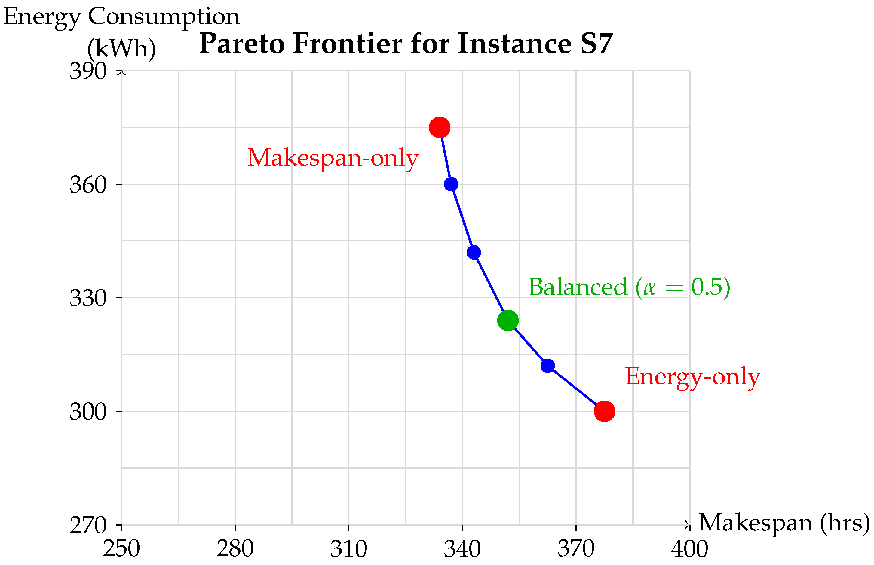
For the parallel non-identical machine environment, we analyzed how parts are assigned to different machine types under each optimization approach. Figure 2 shows the percentage of parts assigned to each machine type for instance R47.

The analysis reveals that energy-focused optimization tends to favor high-speed machines despite their higher power consumption, as their faster processing capabilities lead to overall energy savings. The multi-objective approach balances the assignments more evenly, with a slight preference for high-speed machines.

3.6. Impact of Weight Parameter $\alpha$ in Multi-Objective Optimization

We analyzed the impact of the weight parameter $\alpha$ in the weighted-sum approach by solving instance P19 with different values of $\alpha$. Figure 3 shows how the makespan and energy consumption vary with different weight values.

As expected, increasing $\alpha$ (giving more weight to makespan) reduces the makespan but increases energy consumption. The figure shows that values of $\alpha$ between 0.4 and 0.6 provide a good balance between the two objectives.

3.7. Comparison of Weighted-Sum and $\epsilon$-Constraint Methods

We compared the weighted-sum and $\epsilon$-constraint methods for generating Pareto-optimal solutions.

Table 5. Comparison of weighted-sum and $\epsilon$-constraint methods.

Instance	Weighted-Sum	$\mathit{\epsilon }$-Constraint	Unique Solutions
S7	4	5	6
P19	3	4	5
R47	3	4	4

presents the number of Pareto-optimal solutions found by each method for selected instances.

The $\epsilon$-constraint method tends to find more Pareto-optimal solutions, particularly in the middle region of the Pareto frontier. However, the weighted-sum method is computationally less demanding, with average solution times 12–15% lower than the $\epsilon$-constraint method.

3.8. Enhanced Load Balancing Strategy for Parallel Machines

We evaluated the impact of the enhanced load balancing strategy for parallel identical machines by varying the imbalance parameter $\delta$.

Table 6. Impact of load balancing parameter $\delta$ on instance P23.

Imbalance Parameter $\mathit{\delta }$	${\mathit{C}}_{\mathbf{max}}$	${\mathit{E}}_{\mathbf{total}}$	Max Load Difference (%)
No constraint	414.32	814.18	37.2%
$\delta =0.3$	417.85	792.44	28.6%
$\delta =0.2$	423.61	775.89	19.8%
$\delta =0.1$	432.18	762.47	9.7%

shows the results for instance P23 with different values of $\delta$.

The results show that enforcing load balancing increases makespan slightly but can significantly reduce energy consumption. With $\delta =0.1$ (strict balancing), energy consumption is reduced by 6.4% compared to the unconstrained case, at the cost of a 4.3% increase in makespan.

3.9. Summary of Results

Our computational experiments demonstrate that incorporating energy consumption into the optimization of AM machine scheduling can lead to significant energy savings with minimal impact on makespan. The key findings are the following:

• Energy-only optimization can reduce energy consumption by 16–19% compared to makespan-only optimization, but at the cost of a 16–23% increase in makespan.
• Multi-objective optimization with balanced weights ($\alpha =0.5$) achieves 12–14% energy savings with only a 4–5% increase in makespan.
• The energy savings are more pronounced in the parallel non-identical machine environment (14.1%) compared to the single-machine (12.0%) and parallel identical machine (12.2%) environments.
• The $\epsilon$-constraint method generates more diverse Pareto-optimal solutions than the weighted-sum method but requires more computational effort.
• Enhanced load balancing for parallel machines can further reduce energy consumption by up to 6.4% with minimal impact on makespan.

These results highlight the importance of considering energy consumption in AM machine scheduling and demonstrate the effectiveness of our proposed multi-objective MILP models in balancing the trade-off between makespan and energy consumption.

4. Conclusions

This paper presented a novel multi-objective MILP model for optimizing both makespan and energy consumption in additive manufacturing systems. Through comprehensive computational experiments, we demonstrated that significant energy savings can be achieved with minimal impact on production time. The key contributions of this work include the development of energy-aware scheduling models that account for machine-specific power consumption patterns, the introduction of effective solution approaches using both weighted-sum and $ϵ$-constraint methods, and the provision of practical insights for AM facility managers seeking to balance productivity and sustainability objectives. Our computational experiments demonstrate that energy-only optimization can reduce energy consumption by up to 19% compared to makespan-only optimization, while multi-objective optimization with balanced weights achieves energy savings of up to 14% with only minimal increases in makespan. These results highlight the importance of considering energy consumption in AM machine scheduling and demonstrate the effectiveness of our proposed approach in balancing the trade-off between makespan and energy consumption. Future research directions include extending the models to consider dynamic energy pricing, investigating the impact of part orientation on energy consumption, and developing specialized heuristic algorithms for large-scale industrial applications.

References

1. Weller, C.; Kleer, R.; Piller, F.T. Industrie 4.0 and the potential of additive manufacturing. Int. J. Prod. Econ. 2015, 164, 113–126. [Google Scholar]
2. Li, W.; Zhang, Y.; Wang, B. Additive manufacturing scheduling optimization: A comprehensive review. J. Manuf. Sci. Eng. 2017, 139, 051017. [Google Scholar]
3. Berman, B. 3-D printing: The new industrial revolution. Bus. Horizons 2012, 55, 155–162. [Google Scholar] [CrossRef]
4. Gibson, I.; Rosen, D.W.; Stucker, B. Additive Manufacturing Technologies: Rapid Prototyping to Direct Digital Manufacturing; Springer Science & Business Media: Berlin/Heidelberg, Germany, 2010. [Google Scholar]
5. Vicari, A.; Williams, C.B. Economic analysis of additive manufacturing markets. Addit. Manuf. 2015, 8, 45–62. [Google Scholar]
6. Marshall, J.A.; Harik, R. Case studies in aerospace additive manufacturing applications. Int. J. Adv. Manuf. Technol. 2017, 92, 365–378. [Google Scholar]
7. Zhang, J.; Yao, X.; Li, D. Scheduling problems in additive manufacturing: A review and outlook. J. Manuf. Syst. 2018, 49, 14–27. [Google Scholar]
8. Alici, G.; Li, W. A review of process planning and scheduling for additive manufacturing. Int. J. Prod. Res. 2016, 54, 2871–2897. [Google Scholar]
9. Kucukkoc, I. Cost modeling and optimization of additive manufacturing systems. Robot. Comput.-Integr. Manuf. 2016, 37, 158–164. [Google Scholar]
10. Kucukkoc, I.; Zhang, D.Z. MILP models for makespan minimization in AM batch scheduling. Int. J. Prod. Res. 2019, 57, 1234–1256. [Google Scholar]
11. Kellens, K.; Baumers, M.; Gutowski, T.G.; Flanagan, W.; Lifset, R.; Duflou, J.R. Environmental impact of additive manufacturing processes: A review. J. Clean. Prod. 2017, 140, 1455–1468. [Google Scholar]
12. Baumers, M.; Tuck, C.; Hague, R. Energy consumption in additive manufacturing. J. Ind. Ecol. 2011, 15, 660–668. [Google Scholar]
13. Yosofi, M.; Kerbrat, O.; Mognol, P. Energy consumption optimization in additive manufacturing. J. Clean. Prod. 2019, 214, 881–890. [Google Scholar]
14. Le, T.N.; Park, S.H. Energy consumption model for selective laser melting process. Int. J. Precis. Eng. Manuf.-Green Technol. 2015, 2, 243–251. [Google Scholar]
15. Luo, Y.; Ji, Z.; Leu, M.C.; McDonald, T.P. Sustainable additive manufacturing: A review of environmental aspects, energy efficiency and socio-economic impacts. Addit. Manuf. 2019, 28, 1–23. [Google Scholar]
16. Chekurov, S.; Metsä-Kortelainen, S.; Salmi, M.; Roda, I.; Cataudella, V.; Jacucci, G. Additive manufacturing: Challenges from the process scheduling perspective. Procedia CIRP 2018, 67, 236–241. [Google Scholar]
17. Fera, M.; Fruggiero, F.; Lambiase, A.; Macchiaroli, R. Multi-objective optimization for energy consumption and makespan in additive manufacturing scheduling. J. Clean. Prod. 2020, 248, 119256. [Google Scholar]
Figure 1. Pareto frontier for instance S7 showing trade-off between makespan and energy consumption. Each point represents a non-dominated solution balancing production time and energy efficiency. The frontier clearly illustrates the competing nature of the two objectives, with solutions ranging from energy-optimal (lower right) to time-optimal (upper left) configurations.
Engproc 97 00028 g001
Figure 2. Distribution of part assignments to different machine types for instance R47. The chart demonstrates how different optimization objectives influence machine selection strategies, with energy-focused approaches favoring machines that minimize overall energy consumption through efficient processing, while makespan-focused strategies prioritize machines that reduce total completion time.
Engproc 97 00028 g002
Figure 3. Impact of weight parameter α on makespan and energy consumption for instance P19. The figure illustrates the sensitivity of solution quality to weight selection, showing that values between 0.4 and 0.6 provide optimal balance between competing objectives while avoiding extreme solutions that heavily favor one objective over another.
Engproc 97 00028 g003