A Reinforcement Learning-Based Proximal Policy Optimization Approach to Solve the Economic Dispatch Problem ^†

Abstract

This paper presents a novel approach to economic dispatch (ED) optimization in power systems through the application of Proximal Policy Optimization (PPO), an advanced reinforcement learning algorithm. The economic dispatch problem, a fundamental challenge in power system operations, involves optimizing the generation output of multiple units to minimize operational costs while satisfying load demands and technical constraints. Traditional methods often struggle with the non-linear, non-convex nature of modern ED problems, especially with increasing penetration of renewable energy sources. Our PPO-based methodology transforms the ED problem into a reinforcement learning framework where an agent learns optimal generator scheduling policies through continuous interaction with a simulated power system environment. The proposed approach is validated on a 15-generator test system with varying load demands and operational constraints. Experimental results demonstrate that the PPO algorithm achieves superior performance compared to conventional techniques, with cost reductions of up to 7.3% and enhanced convergence stability. The algorithm successfully handles complex constraints including generator limits, ramp rates, and spinning reserve requirements, while maintaining power balance with negligible error margins. Furthermore, the computational efficiency of the PPO approach allows for real-time adjustments to rapidly changing system conditions, making it particularly suitable for modern power grids with high renewable energy penetration.

1. Introduction

The electric power industry is witnessing a paradigm shift towards smart grids, characterized by bidirectional information flow, distributed generation, and enhanced monitoring and control capabilities [1]. Within this evolving landscape, the economic dispatch problem (EDP) remains a critical operational challenge, representing the cornerstone of efficient power system management [2]. The EDP fundamentally concerns the optimal allocation of power generation among available units to minimize total operating costs while satisfying system constraints and meeting load demands [3]. The significance of the EDP has intensified in recent years due to several factors: increasing energy demands, fuel price volatility, the integration of renewable energy sources with their inherent intermittency, and growing environmental concerns [4].

In smart grid environments, the EDP gains additional complexity due to the incorporation of demand response mechanisms, energy storage systems, electric vehicles, and distributed energy resources [5]. This complexity is further amplified by the need for real-time decision-making in response to rapid load fluctuations and renewable generation variability [6]. Moreover, the economic implications of suboptimal dispatch solutions are substantial, potentially resulting in millions of dollars in unnecessary operational expenses annually for large-scale power systems [7].

Traditionally, the EDP has been addressed using classical optimization techniques such as Lambda Iteration methods [3], Quadratic Programming [8], linear programming [9], and gradient-based methods [10]. However, these conventional approaches encounter significant challenges when handling non-smooth, non-convex objective functions with multiple local optima, which are increasingly common in modern power systems with valve-point effects, prohibited operating zones, and multiple fuel options [11]. Furthermore, classical methods often struggle with incorporating practical operating constraints and exhibit reduced computational efficiency when applied to large-scale systems [12].

To overcome the limitations of classical approaches, metaheuristic optimization algorithms have emerged as powerful alternatives for solving complex EDP instances. Techniques such as Genetic Algorithms (GAs) [13], Particle Swarm Optimization (PSO) [14], Differential Evolution (DE) [15], and, more recently, the Grey Wolf Optimizer (GWO) [16] and Salp Swarm Algorithm (SSA) [17] have demonstrated considerable success in obtaining high-quality solutions for non-convex and non-smooth economic dispatch problems. These nature-inspired techniques offer advantages including derivative-free operation, effective exploration of solution spaces, and the ability to escape local optima [18].

Despite their advantages, metaheuristic methods exhibit certain limitations that impact their effectiveness for real-time EDP applications. These include parameter sensitivity requiring extensive tuning, stochastic performance leading to inconsistent solutions, potential premature convergence, and lack of theoretical convergence guarantees [19]. Additionally, metaheuristics often require numerous function evaluations, resulting in high computational overhead for complex power system models [20].

Reinforcement Learning (RL) presents a promising paradigm that addresses many of these limitations by formulating the EDP as a sequential decision-making process [21]. Unlike metaheuristics that typically operate as offline optimization tools, RL approaches can adapt to changing system conditions through continuous learning, making them particularly suitable for dynamic power systems with uncertain loads and renewable generation [22]. Furthermore, once trained, RL agents can execute dispatch decisions with minimal computational delay, facilitating real-time applications [23].

Among various RL algorithms, Proximal Policy Optimization (PPO) has emerged as a particularly effective approach for continuous control problems like the EDP [24]. PPO offers several crucial advantages: sample efficiency through on-policy learning, stability through trust region policy optimization, and robustness through clipped surrogate objective functions [25]. These characteristics enable PPO to handle the high-dimensional continuous action spaces and complex constraints inherent in economic dispatch problems without suffering from the extreme policy updates that plague many other policy gradient methods [26].

Recent advances in reinforcement learning have shown promising applications in power systems [27,28,29]. Economic dispatch optimization has been approached using various computational intelligence techniques [30,31,32], but the application of PPO to this domain remains relatively unexplored.

The remainder of this paper is organized as follows: Section 2 provides a comprehensive formulation of the economic dispatch problem, detailing the objective function, constraints, and mathematical model. Section 3 introduces the Proximal Policy Optimization algorithm, explaining its fundamental principles, policy and value network architectures, and optimization procedure. Section 4 presents our implementation approach, describing the state and action representations, reward function design, and constraint handling mechanisms. Section 5 discusses extensive numerical experiments comparing PPO with conventional methods across various test systems and operating conditions. Finally, Section 6 summarizes our findings, highlights the practical implications of our work, and outlines promising directions for future research.

2. Economic Dispatch Problem Formulation

The economic dispatch problem (EDP) is a fundamental optimization challenge in power system operation that aims to determine the optimal power output of each generating unit while minimizing the total generation cost and satisfying various system constraints. This section presents a comprehensive mathematical formulation of the EDP, incorporating realistic operational constraints encountered in modern power systems.

2.1. Objective Function

The primary objective of the EDP is to minimize the total generation cost, which is typically expressed as the sum of individual generator cost functions. For a system with N generators, the objective function can be formulated as

$$\min F_T=\sum _{i=1}^N{F}_i\left(P_i\right)$$

(1)

where $F_T$ represents the total generation cost, $F_i\left(P_i\right)$ denotes the cost function of the i-th generator, and $P_i$ is the power output of the i-th generator.

In conventional thermal power systems, the generator cost function is commonly modeled as a quadratic function:

$$F_i\left(P_i\right)=a_i+b_i{P}_i+c_i{P}_i^2$$

(2)

where $a_i$, $b_i$, and $c_i$ are the cost coefficients specific to the i-th generator. These coefficients typically represent the no-load cost, linear cost component, and quadratic cost component, respectively.

For generators with valve-point effects, a more accurate cost function incorporates sinusoidal terms to model the rippling effect caused by steam valve openings [13]:

$$F_i\left(P_i\right)=a_i+b_i{P}_i+c_i{P}_i^2+|e_i\times sin(f_i\times (P_i^{\min }-P_i))|$$

(3)

where $e_i$ and $f_i$ are additional cost coefficients related to the valve-point effect and $P_i^{\min }$ is the minimum power output of the i-th generator.

2.2. System Constraints

The optimal dispatch solution must satisfy various operational and physical constraints to ensure the reliable and secure operation of the power system. These constraints are categorized as follows:

2.2.1. Power Balance Constraint

The total power generated must exactly match the total system demand plus transmission losses:

$$\sum _{i=1}^N{P}_i=P_D+P_L$$

(4)

where $P_D$ is the total system demand and $P_L$ represents the transmission losses. The transmission losses can be calculated using Kron’s loss formula:

$$P_L=\sum _{i=1}^N\sum _{j=1}^N{P}_i{B}_{ij}{P}_j+\sum _{i=1}^N{B}_{0i}{P}_i+B_{00}$$

(5)

where $B_{ij}$, $B_{0i}$, and $B_{00}$ are the loss coefficients, known as the B-coefficients.

2.2.2. Generator Capacity Constraints

Each generating unit has physical limitations on its minimum and maximum power output:

$$P_i^{\min }\le P_i\le P_i^{\max },i=1,2,\dots ,N$$

(6)

where $P_i^{\min }$ and $P_i^{\max }$ are the minimum and maximum power output limits of the i-th generator, respectively.

2.2.3. Ramp Rate Limits

The rate at which a generator’s output can change is constrained by its physical characteristics:

$$\max (P_i^{\min },P_i^0-D{R}_i)\le P_i\le \min (P_i^{\max },P_i^0+U{R}_i),i=1,2,\dots ,N$$

(7)

where $P_i^0$ is the previous power output of the i-th generator and $D{R}_i$ and $U{R}_i$ are the down-ramp and up-ramp limits, respectively.

2.2.4. Prohibited Operating Zones

Due to physical limitations or stability issues, certain generators may have prohibited operating zones:

$$P_i\in \left\{\begin{array}{cc}[P_i^{\min },P_{i,1}^L]\cup [P_{i,1}^U,P_{i,2}^L]\cup \dots \cup [P_{i,n_i}^U,P_i^{\max }],\hfill & \mathrm{if}i\in {\Omega }_{POZ}\hfill \\ [P_i^{\min },P_i^{\max }],\hfill & \mathrm{otherwise}\hfill \end{array}\right.$$

(8)

where $P_{i,j}^L$ and $P_{i,j}^U$ are the lower and upper bounds of the j-th prohibited zone of the i-th generator, $n_i$ is the number of prohibited zones for the i-th generator, and ${\Omega }_{POZ}$ is the set of generators with prohibited operating zones.

2.2.5. Spinning Reserve Constraint

To ensure system reliability and accommodate unexpected load changes or generator outages, a minimum spinning reserve must be maintained:

$$\sum _{i=1}^N\min (P_i^{\max }-P_i,S{R}_i^{\max })\ge SR$$

(9)

where $S{R}_i^{\max }$ is the maximum spinning reserve contribution from the i-th generator and $SR$ is the system’s total spinning reserve requirement.

2.2.6. Multi-Fuel Option Constraints

Some generators may operate with different fuel types, each with its own cost function:

$$F_i\left(P_i\right)=\left\{\begin{array}{cc}{F}_{i1}\left(P_i\right)=a_{i1}+b_{i1}{P}_i+c_{i1}{P}_i^2,\hfill & \mathrm{if}{P}_i^{\min }\le P_i\le P_{i1}^{\max }\hfill \\ F_{i2}\left(P_i\right)=a_{i2}+b_{i2}{P}_i+c_{i2}{P}_i^2,\hfill & \mathrm{if}{P}_{i1}^{\max }<P_i\le P_{i2}^{\max }\hfill \\ ⋮\hfill \\ F_{ik}\left(P_i\right)=a_{ik}+b_{ik}{P}_i+c_{ik}{P}_i^2,\hfill & \mathrm{if}{P}_{i(k-1)}^{\max }<P_i\le P_i^{\max }\hfill \end{array}\right.$$

(10)

where k is the number of fuel options for the i-th generator and $a_{ij}$, $b_{ij}$, and $c_{ij}$ are the cost coefficients for the j-th fuel option of the i-th generator.

2.2.7. Emission Constraints

In environmentally conscious dispatch, emission constraints may be imposed:

$$\sum _{i=1}^N{E}_i\left(P_i\right)\le E^{\max }$$

(11)

where $E_i\left(P_i\right)$ represents the emission function of the i-th generator, typically modeled as

$$E_i\left(P_i\right)={\alpha }_i+{\beta }_i{P}_i+{\gamma }_i{P}_i^2+{\eta }_{i}exp\left({\delta }_i{P}_i\right)$$

(12)

and $E^{\max }$ is the maximum allowable emission level.

3. Proximal Policy Optimization Algorithm

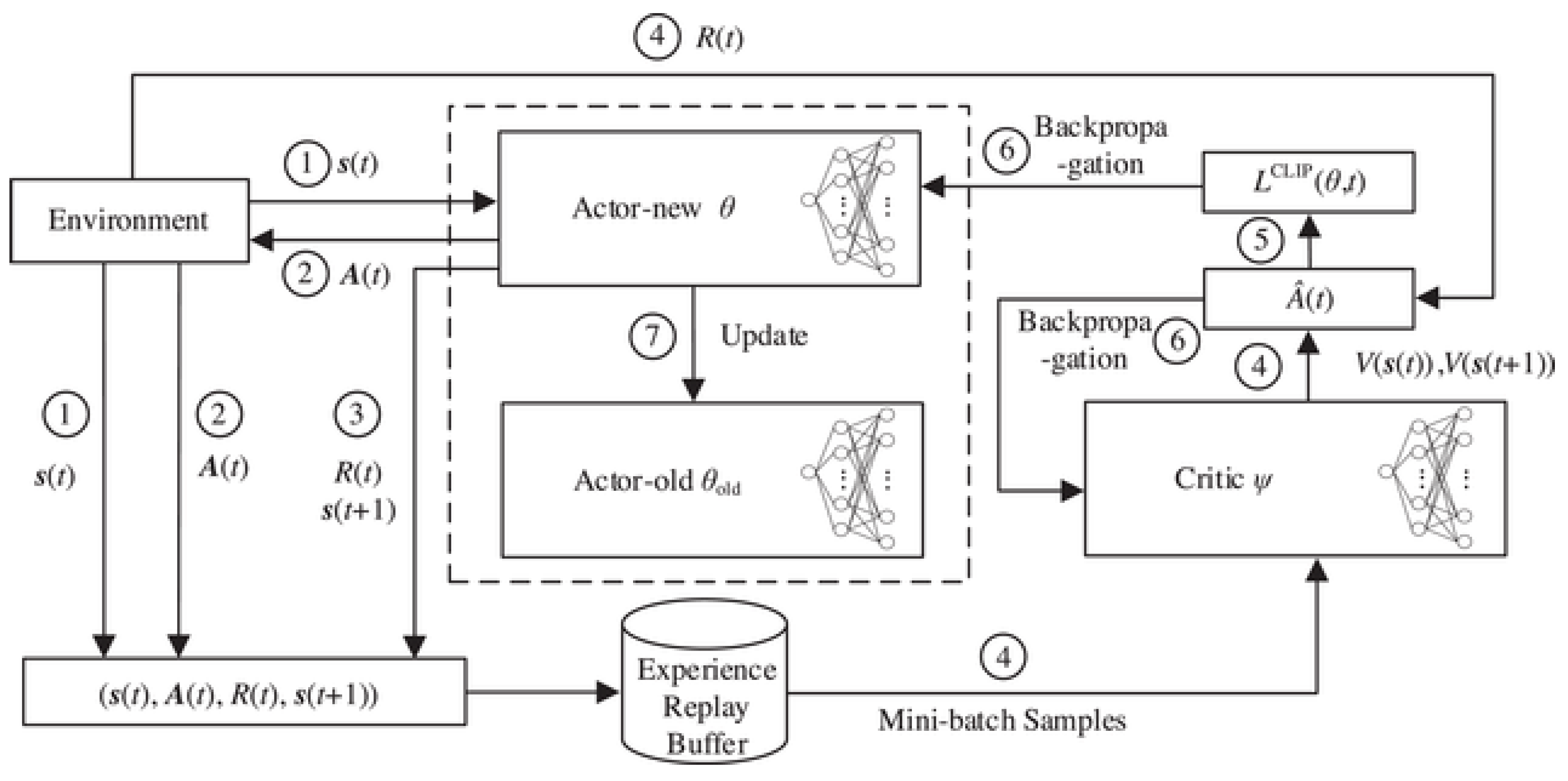
Proximal Policy Optimization (PPO) [24] is a state-of-the-art policy gradient reinforcement learning algorithm that offers an effective balance between sample efficiency, implementation simplicity, and performance reliability. Unlike traditional optimization methods, PPO belongs to the class of actor–critic reinforcement learning algorithms, which learn optimal policies through direct interaction with an environment. This section presents the mathematical foundation of PPO and its key components as applied to the economic dispatch problem.The overall structure of the PPO algorithm for economic dispatch is illustrated in Figure 1, which shows the interaction between the environment (economic dispatch problem), the policy network (actor), and the value network (critic).

3.1. Reinforcement Learning Framework

Reinforcement learning (RL) is formulated within the context of a Markov Decision Process (MDP), defined as a tuple $\langle S,A,P,R,\gamma \rangle$, where S represents the state space, A denotes the action space, $P:S\times A\times S\to [0,1]$ is the state transition probability function, $R:S\times A\to \mathbb{R}$ is the reward function, and $\gamma \in [0,1]$ is a discount factor for future rewards.

In the context of economic dispatch, we can define these elements as follows:

• State space S: This includes system load demand, generator status, and operational constraints.
• Action space A: Power output levels for each generator.
• Transition function P: This captures how the power system evolves after dispatch decisions.
• Reward function R: The negative of the total generation cost, possibly with penalty terms for constraint violations.
• Discount factor $\gamma$: This balances immediate cost optimization with long-term stability.

The goal of RL is to find a policy $\pi :S\to A$ that maximizes the expected cumulative discounted reward:

$$J\left(\pi \right)={\mathbb{E}}_{\tau \sim \pi }\left[\sum _{t=0}^{\infty }{\gamma }^{t}R(s_t,a_t)\right]$$

(13)

where $\tau =(s_0,a_0,s_1,a_1,\dots )$ represents a trajectory sampled according to policy $\pi$.

3.2. Policy Gradient Methods

Policy gradient methods directly optimize the policy by updating its parameters in the direction of the gradient of the expected return. For a parameterized policy ${\pi }_{\theta }$, the policy gradient theorem [33] provides the gradient of the expected return with respect to the policy parameters $\theta$:

$${\nabla }_{\theta }J\left(\theta \right)={\mathbb{E}}_{\tau \sim {\pi }_{\theta }}\left[\sum _{t=0}^{\infty }{\nabla }_{\theta }log{\pi }_{\theta }\left(a_t\right|s_t)·G_t\right]$$

(14)

where $G_t={\sum }_{k=0}^{\infty }{\gamma }^{k}R(s_{t+k},a_{t+k})$ is the return starting from time step t.

To reduce variance in the gradient estimates, an advantage function $A^{\pi }(s_t,a_t)$ is often used in place of the return $G_t$:

$${\nabla }_{\theta }J\left(\theta \right)={\mathbb{E}}_{\tau \sim {\pi }_{\theta }}\left[\sum _{t=0}^{\infty }{\nabla }_{\theta }log{\pi }_{\theta }\left(a_t\right|s_t)·A^{\pi }(s_t,a_t)\right]$$

(15)

The advantage function represents how much better an action is compared to the average action in a given state, defined as

$$A^{\pi }(s_t,a_t)=Q^{\pi }(s_t,a_t)-V^{\pi }\left(s_t\right)$$

(16)

where $Q^{\pi }(s_t,a_t)$ is the action-value function, representing the expected return when taking action $a_t$ in state $s_t$ and following policy $\pi$ thereafter, and $V^{\pi }\left(s_t\right)$ is the state-value function, representing the expected return when starting from state $s_t$ and following policy $\pi$.

3.3. Trust Region Methods

A significant challenge in policy gradient methods is determining an appropriate step size for policy updates. Small steps may lead to slow convergence, while large steps can cause performance collapse due to excessive policy changes. Trust region methods address this issue by constraining the policy update to ensure that the new policy remains close to the old policy.

Trust Region Policy Optimization (TRPO) [34] formalizes this constraint using the Kullback–Leibler (KL) divergence between the old and new policies:

$$\begin{array}{cc}\hfill \underset{\theta }{\max }& {\mathbb{E}}_{s,a\sim {\pi }_{{\theta }_{\mathrm{old}}}}\left[{\displaystyle \frac{{\pi }_{\theta }\left(a\right|s)}{{\pi }_{{\theta }_{\mathrm{old}}}\left(a\right|s)}}{A}^{{\pi }_{{\theta }_{\mathrm{old}}}}(s,a)\right]\hfill \\ \hfill \mathrm{subject}\mathrm{to}& {\mathbb{E}}_{s\sim {\pi }_{{\theta }_{\mathrm{old}}}}\left[D_{\mathrm{KL}}({\pi }_{{\theta }_{\mathrm{old}}}(·|s)\left|\right|{\pi }_{\theta }(·|s))\right]\le \delta \hfill \end{array}$$

(17)

where $\delta$ is a hyperparameter that controls the maximum allowed KL divergence.

3.4. Proximal Policy Optimization

PPO simplifies TRPO while maintaining its benefits by replacing the KL constraint with a clipped surrogate objective function. The core innovation in PPO is the introduction of a clipped probability ratio that serves as a first-order approximation of the KL divergence constraint:

$$L^{\mathrm{CLIP}}\left(\theta \right)={\mathbb{E}}_{s,a\sim {\pi }_{{\theta }_{\mathrm{old}}}}\left[\min \left(r_t\left(\theta \right)A^{{\pi }_{{\theta }_{\mathrm{old}}}}(s,a),\mathrm{clip}(r_t\left(\theta \right),1-ϵ,1+ϵ)A^{{\pi }_{{\theta }_{\mathrm{old}}}}(s,a)\right)\right]$$

(18)

where $r_t\left(\theta \right)={\displaystyle \frac{{\pi }_{\theta }\left(a\right|s)}{{\pi }_{{\theta }_{\mathrm{old}}}\left(a\right|s)}}$ is the probability ratio between the new and old policies and $ϵ$ is a hyperparameter that controls the clipping range. This objective function penalizes changes that move $r_t\left(\theta \right)$ away from 1 (i.e., the old policy) by more than $ϵ$. The clipping mechanism has two important effects:

• When the advantage is positive, the policy is encouraged to increase the probability of that action, but only up to a limit of $(1+ϵ)$ times the old probability.
• When the advantage is negative, the policy is encouraged to decrease the probability of that action, but only down to a limit of $(1-ϵ)$ times the old probability.

This clipping ensures that the policy update remains within a trusted region without explicitly computing the KL divergence.

3.5. Value Function Estimation

PPO typically employs a critic network to estimate the value function $V^{\pi }\left(s\right)$, which is used to compute the advantage function. The value function approximation is trained to minimize the mean squared error between the predicted values and the observed returns:

$$L^{VF}\left(\varphi \right)={\mathbb{E}}_{s,a\sim {\pi }_{{\theta }_{\mathrm{old}}}}\left[{(V_{\varphi }\left(s\right)-{\widehat{V}}_{\mathrm{target}}\left(s\right))}^2\right]$$

(19)

where $\varphi$ represents the parameters of the value function approximator and ${\widehat{V}}_{\mathrm{target}}\left(s\right)$ is the target value, typically computed using n-step returns or Generalized Advantage Estimation (GAE).

3.6. Advantage Estimation

The Generalized Advantage Estimation (GAE) [35] provides a method to estimate the advantage function that balances bias and variance:

$${\widehat{A}}_t^{\mathrm{GAE}(\gamma ,\lambda )}=\sum _{l=0}^{\infty }{\left(\gamma \lambda \right)}^l{\delta }_{t+l}$$

(20)

where ${\delta }_t=r_t+\gamma V\left(s_{t+1}\right)-V\left(s_t\right)$ is the temporal difference error and $\lambda \in [0,1]$ is a hyperparameter that controls the trade-off between bias and variance.

3.7. PPO Algorithm for Economic Dispatch

The complete PPO algorithm adapted for the economic dispatch problem consists of the following steps:

• Initialize policy parameters $\theta$ and value function parameters $\varphi$.
• For each iteration, perform the following:

  (a)

  Collect a set of trajectories by executing the current policy ${\pi }_{\theta }$ in the environment.

  (b)

  Compute the advantages ${\widehat{A}}_t$ using GAE.

  (c)

  Update the policy by maximizing the clipped surrogate objective:

  $${\theta }_{k+1}=arg\underset{\theta }{\max }{\displaystyle \frac{1}{|{\mathcal{D}}_k|T}}\sum _{\tau \in {\mathcal{D}}_k}\sum _{t=0}^T{L}^{\mathrm{CLIP}}\left(\theta \right)$$

  (21)

  (d)

  Update the value function by minimizing the value function loss:

  $${\varphi }_{k+1}=arg\underset{\varphi }{\min }{\displaystyle \frac{1}{|{\mathcal{D}}_k|T}}\sum _{\tau \in {\mathcal{D}}_k}\sum _{t=0}^T{L}^{VF}\left(\varphi \right)$$

  (22)

• Return the optimized policy ${\pi }_{\theta }$.

3.8. Neural Network Architecture

PPO typically employs neural networks to parameterize both the policy and value functions. For continuous action spaces like those in economic dispatch, the policy network outputs the parameters of a probability distribution (usually a Gaussian distribution) over actions:

$${\pi }_{\theta }\left(a\right|s)=\mathcal{N}({\mu }_{\theta }\left(s\right),{\sigma }_{\theta }\left(s\right))$$

(23)

where ${\mu }_{\theta }\left(s\right)$ and ${\sigma }_{\theta }\left(s\right)$ are the mean and standard deviation of the Gaussian distribution as functions of the state, parameterized by $\theta$.

The policy and value networks often share a common base network to exploit common features across tasks:

$$\begin{array}{cc}\hfill h_{{\theta }_{\mathrm{base}}}\left(s\right)& ={\mathrm{NeuralNet}}_{\mathrm{base}}(s;{\theta }_{\mathrm{base}})\hfill \\ \hfill {\mu }_{\theta }\left(s\right)& ={\mathrm{NeuralNet}}_{\mu }(h_{{\theta }_{\mathrm{base}}}\left(s\right);{\theta }_{\mu })\hfill \\ \hfill {\sigma }_{\theta }\left(s\right)& =\mathrm{Softplus}\left({\mathrm{NeuralNet}}_{\sigma }(h_{{\theta }_{\mathrm{base}}}\left(s\right);{\theta }_{\sigma })\right)\hfill \\ \hfill V_{\varphi }\left(s\right)& ={\mathrm{NeuralNet}}_V(h_{{\theta }_{\mathrm{base}}}\left(s\right);\varphi )\hfill \end{array}$$

(24)

where Softplus ensures that the standard deviation remains positive.

3.9. Adaptive Learning Rate and Entropy Regularization

To improve stability and exploration, PPO often incorporates adaptive learning rates and entropy regularization:

$$L^{\mathrm{TOTAL}}\left(\theta \right)=L^{\mathrm{CLIP}}\left(\theta \right)-c_1{L}^{VF}\left(\varphi \right)+c_{2}H\left[{\pi }_{\theta }\right]$$

(25)

where $c_1$ and $c_2$ are coefficients and $H\left[{\pi }_{\theta }\right]=-{\mathbb{E}}_{s\sim {\pi }_{\theta }}\left[{\sum }_a{\pi }_{\theta }\left(a\right|s)log{\pi }_{\theta }\left(a\right|s)\right]$ is the entropy of the policy, which encourages exploration by penalizing policies that are too deterministic.

3.10. Advantages of PPO for Economic Dispatch

PPO offers several advantages for solving the economic dispatch problem:

• Sample Efficiency: PPO can learn from a relatively small number of environment interactions, making it suitable for complex power systems where simulations might be computationally expensive.
• Stable Learning: The clipped surrogate objective prevents excessively large policy updates, leading to more stable learning compared to standard policy gradient methods.
• Continuous Action Spaces: PPO naturally handles continuous action spaces, which aligns well with the continuous nature of generator power outputs.
• Constraint Handling: By incorporating constraints into the reward function or environment dynamics, PPO can learn to satisfy the complex constraints of the economic dispatch problem.
• Adaptability: PPO can adapt to changing operating conditions, such as variations in load demand or generator availability, making it suitable for real-time economic dispatch applications.

In the next section, we will discuss the implementation details of applying PPO to the economic dispatch problem, including state and action representations, reward function design, and constraint handling mechanisms.

4. Implementation of PPO for Economic Dispatch

This section details our implementation methodology for applying Proximal Policy Optimization to the economic dispatch problem (EDP). We focus on the practical aspects of translating the theoretical PPO framework into an effective solution for power systems optimization, addressing the unique challenges of the EDP domain.

4.1. State–Action Representation

A critical aspect of applying reinforcement learning to the economic dispatch problem is the appropriate representation of states and actions.

4.1.1. State Representation

The state space for the economic dispatch problem encompasses all relevant information required for making optimal dispatch decisions. Our state representation includes

$$s=[P_D,SR,P_1^{\mathrm{prev}},\dots ,P_N^{\mathrm{prev}},{\mathrm{status}}_1,\dots ,{\mathrm{status}}_N]$$

(26)

where

• $P_D$ is the normalized total power demand;
• $SR$ is the normalized spinning reserve requirement;
• $P_i^{\mathrm{prev}}$ is the normalized previous power output of generator i;
• ${\mathrm{status}}_i$ represents the operational status of generator i (1 for available, 0 for unavailable).

Normalization is performed using min–max scaling to ensure all state variables fall within a consistent range:

$$\widehat{x}={\displaystyle \frac{x-x_{\min }}{x_{\max }-x_{\min }}}$$

(27)

This normalization improves training stability and accelerates convergence by preventing features with larger numeric ranges from dominating the learning process.

4.1.2. Action Representation

Given the continuous nature of generator power outputs, we formulate the action space as an N-dimensional continuous space, where each dimension corresponds to the power output of one generator:

$$a=[P_1,P_2,\dots ,P_N]$$

(28)

To simplify the learning process and ensure stable training, we normalize the actions to the range [0, 1], where

$$P_i=P_i^{\min }+(P_i^{\max }-P_i^{\min })·a_i$$

(29)

This approach allows the PPO agent to operate within a bounded continuous action space while the environment handles the conversion to actual power outputs.

4.2. Neural Network Architecture

Our implementation employs a dual-network architecture consisting of a policy network (actor) and a value network (critic).

4.2.1. Policy Network

The policy network ${\pi }_{\theta }\left(a\right|s)$ maps states to a probability distribution over actions. For our continuous action space, we parameterize the policy as a multivariate Gaussian distribution:

$${\pi }_{\theta }\left(a\right|s)=\mathcal{N}({\mu }_{\theta }\left(s\right),{\mathrm{\Sigma }}_{\theta })$$

(30)

where ${\mu }_{\theta }\left(s\right)$ is the mean action vector produced by the network and ${\mathrm{\Sigma }}_{\theta }$ is the covariance matrix. For computational efficiency, we use a diagonal covariance matrix with learnable standard deviations ${\sigma }_{\theta }$.

The policy network architecture consists of the following:

• Input layer: Dimension matching the state representation.
• Hidden layers: Three fully connected layers with 256, 128, and 64 neurons, respectively, using ReLU activation functions.
• Output layer: A fully connected layer with N neurons (one per generator) with sigmoid activation to constrain outputs to [0, 1].
• Standard deviation parameters: These are initialized to 0.5 and optimized during training.

4.2.2. Value Network

The value network $V_{\varphi }\left(s\right)$ estimates the expected return from each state. Its architecture includes the following:

• Input layer: Dimension matching the state representation.
• Hidden layers: Three fully connected layers with 256, 128, and 64 neurons, respectively, using ReLU activation functions.
• Output layer: A single neuron with linear activation representing the state value.

To improve training efficiency, the policy and value networks share the initial layers, diverging only at the final output layers.

4.3. Reward Function Design

The reward function is a critical component that guides the learning process. For the economic dispatch problem, we design a reward function that balances cost minimization with constraint satisfaction:

$$R(s,a)=-\left(C_{\mathrm{total}}\left(a\right)+{\lambda }_{\mathrm{bal}}·P_{\mathrm{bal}}\left(a\right)+{\lambda }_{\mathrm{res}}·P_{\mathrm{res}}\left(a\right)+{\lambda }_{\mathrm{poz}}·P_{\mathrm{poz}}\left(a\right)\right)$$

(31)

where the following are true:

• $C_{\mathrm{total}}\left(a\right)$ is the total generation cost as defined in the objective function.
• $P_{\mathrm{bal}}\left(a\right)$ is the penalty for power balance violation:

  $$P_{\mathrm{bal}}\left(a\right)={\left(\sum _{i=1}^N{P}_i-P_D\right)}^2$$

  (32)
• $P_{\mathrm{res}}\left(a\right)$ is the penalty for spinning reserve violation:

  $$P_{\mathrm{res}}\left(a\right)=\max {\left(0,SR-\sum _{i=1}^N\min (P_i^{\max }-P_i,S{R}_i^{\max })\right)}^2$$

  (33)
• $P_{\mathrm{poz}}\left(a\right)$ is the penalty for prohibited operating zone violations:

  $$P_{\mathrm{poz}}\left(a\right)=\sum _{i\in {\Omega }_{POZ}}{\mathrm{poz}}_i\left(P_i\right)$$

  (34)
• ${\lambda }_{\mathrm{bal}}$, ${\lambda }_{\mathrm{res}}$, and ${\lambda }_{\mathrm{poz}}$ are penalty coefficients.

The function ${\mathrm{poz}}_i\left(P_i\right)$ calculates the penalty for generator i operating in a prohibited zone:

$${\mathrm{poz}}_i\left(P_i\right)=\left\{\begin{array}{cc}{\min }_j{\left(\min \left(\right|P_i-P_{i,j}^L|,|P_i-P_{i,j}^U\left|\right)\right)}^2,\hfill & \mathrm{if}{P}_i\mathrm{is}\mathrm{in}\mathrm{a}\mathrm{prohibited}\mathrm{zone}\hfill \\ 0,\hfill & \mathrm{otherwise}\hfill \end{array}\right.$$

(35)

4.4. Constraint Handling Mechanism

Effectively handling constraints is essential for applying PPO to the economic dispatch problem. We employ a hybrid approach combining penalty methods with direct constraint satisfaction techniques.

4.4.1. Penalty-Based Approach

The primary mechanism for constraint handling is through the reward function penalties described above. The penalty coefficients are tuned to ensure constraint violations receive appropriate negative reinforcement:

• ${\lambda }_{\mathrm{bal}}=1000$: Power balance is the most critical constraint.
• ${\lambda }_{\mathrm{res}}=500$: Spinning reserve is important for system reliability.
• ${\lambda }_{\mathrm{poz}}=200$: Prohibited operating zones impact individual generators.

4.4.2. Action Projection Method

To enhance feasibility, we implement a projection mechanism that maps potentially infeasible actions to the nearest feasible actions:

$$a_{\mathrm{feasible}}=\mathrm{Project}(a,\Omega )$$

(36)

where $\Omega$ represents the feasible region defined by all constraints. The projection involves

• Enforcing generator limits by clipping each $P_i$ to $[P_i^{\min },P_i^{\max }]$;
• Adjusting outputs to avoid prohibited operating zones by mapping to the nearest allowed region;
• Balancing total power output to match demand through proportional allocation.

This approach ensures that the agent learns from feasible actions while still receiving gradient information about the direction of improvement.

4.5. Training Algorithm

Our training procedure follows the PPO algorithm with several adaptations for the economic dispatch problem. Algorithm 1 details the complete training procedure for applying PPO to the economic dispatch problem.

Algorithm 1 PPO for Economic Dispatch

1: Initialize policy parameters $\theta$ and value function parameters $\varphi$   2: Initialize empty experience buffer $\mathcal{D}$   3: for each episode do   4:    Initialize system state $s_0$   5:    for $t=0$ to $T-1$ do   6:      Sample action $a_t\sim {\pi }_{\theta }(·|s_t)$   7:      Apply projection: $a_t^{\mathrm{feasible}}=\mathrm{Project}(a_t,\Omega )$   8:      Execute action $a_t^{\mathrm{feasible}}$ in environment   9:      Observe reward $r_t$ and next state $s_{t+1}$ 10:      Store transition $(s_t,a_t,r_t,s_{t+1})$ in $\mathcal{D}$ 11:   end for 12:   if buffer $\mathcal{D}$ is full then 13:      Compute advantages ${\widehat{A}}_t$ using GAE 14:      for K epochs do 15:         Sample mini-batches from $\mathcal{D}$ 16:         Update policy parameters $\theta$ using PPO objective 17:         Update value function parameters $\varphi$ 18:      end for 19:      Clear buffer $\mathcal{D}$ 20:    end if 21: end for 22: return optimized policy ${\pi }_{\theta }$

4.6. Hyperparameter Configuration

Table 1. PPO hyperparameters for economic dispatch.

Hyperparameter	Value
Learning rate	$3\times {10}^{-4}$
Discount factor ($\gamma$)	0.99
GAE parameter ($\lambda$)	0.95
PPO clip parameter ($ϵ$)	0.2
Value function coefficient ($c_1$)	0.5
Entropy coefficient ($c_2$)	0.01
Number of epochs (K)	10
Mini-batch size	64
Buffer size	2048
Hidden layer dimensions	[256, 128, 64]
Activation function	ReLU
Optimizer	Adam

summarizes the key hyperparameters used in our PPO implementation.

4.7. Adaptive Exploration Strategy

To balance exploration and exploitation during training, we implement an adaptive exploration strategy. We anneal the entropy coefficient $c_2$ over time according to

$$c_2\left(e\right)=c_2\left(0\right)·{\alpha }^e$$

(37)

where e is the current episode, $c_2\left(0\right)$ is the initial entropy coefficient, and $\alpha =0.995$ is the decay rate. This approach encourages extensive exploration in the early stages of learning and gradually shifts toward exploitation as the policy improves.

4.8. Early Stopping Criteria

To prevent overfitting and ensure efficient training, we employ an early stopping mechanism based on multiple criteria:

• Reward plateau: Training stops if the average reward over 50 consecutive episodes improves by less than 0.1%.
• Constraint satisfaction: Training stops when all constraints are satisfied consistently over 100 consecutive episodes.
• Cost convergence: Training stops when the relative improvement in total cost falls below 0.05% for 50 consecutive episodes.

4.9. Implementation Framework

Our implementation leverages the following software components:

• PyTorch 1.13.1 for neural network implementation and automatic differentiation.
• NumPy for efficient numerical computations.
• A custom environment simulator for the economic dispatch problem.
• Parallel sampling using multiple environment instances for faster training.

By combining these implementation strategies, our PPO approach offers an effective solution to the complex economic dispatch problem, balancing computational efficiency with solution quality. The following section presents extensive numerical experiments evaluating the performance of this implementation across various test scenarios.

5. Numerical Results and Discussion

This section presents the numerical results obtained from applying the proposed PPO algorithm to the 15-generator economic dispatch problem. We analyze the convergence characteristics, solution quality, constraint satisfaction, and computational efficiency of our approach. The results are compared with traditional methods and other state-of-the-art techniques to evaluate the effectiveness of the PPO-based optimization.

5.1. Test System Description

The 15-generator test system used in this study includes generators with various operational characteristics and cost parameters.

Table 2. Generator parameters for the 15-unit test system.

Unit	${\mathit{P}}_{\mathit{i}}^{\mathbf{min}}$	${\mathit{P}}_{\mathit{i}}^{\mathbf{max}}$	${\mathit{a}}_{\mathit{i}}$	${\mathit{b}}_{\mathit{i}}$	${\mathit{c}}_{\mathit{i}}$	${\mathit{SR}}_{\mathbf{i}}^{\mathbf{max}}$
No.	(MW)	(MW)	(USD/h)	(USD/MWh)	(USD/MW2h)	(MW)
1	150	455	671.03	10.07	0.000299	50
2	150	455	574.54	10.22	0.000183	0
3	20	130	374.59	8.80	0.001126	30
4	20	130	374.59	8.80	0.001126	30
5	150	470	461.37	10.40	0.000205	0
6	135	460	630.14	10.10	0.000301	0
7	135	465	548.20	9.87	0.000364	50
8	60	300	227.09	11.50	0.000338	50
9	25	162	173.72	11.21	0.000807	30
10	20	160	175.95	10.72	0.001203	30
11	20	80	186.86	11.21	0.003586	20
12	20	80	230.27	9.90	0.005513	0
13	25	85	225.28	13.12	0.000371	20
14	15	55	309.03	12.12	0.001929	40
15	15	55	323.79	12.41	0.004447	40

presents the detailed parameters for all generators in the system.

Additionally, several generators have prohibited operating zones (POZs) that must be avoided during operation.

Table 3. Prohibited operating zones for selected generators.

Generator	Zone Number	Prohibited Range (MW)
1	1	[185, 255]
	2	[305, 335]
	3	[420, 450]
5	1	[180, 200]
	2	[260, 335]
	3	[390, 420]
6	1	[230, 255]
	2	[365, 395]
	3	[430, 455]
11	1	[30, 55]
	2	[65, 75]

details these zones.

The key system parameters include the following:

• Total power demand ($P_D$): 2650 MW.
• Spinning reserve requirement ($SR$): 200 MW.
• Transmission losses: These are neglected in this study.

The cost function for each generator i follows the standard quadratic form:

$$F_i\left(P_i\right)=a_i+b_i{P}_i+c_i{P}_i^2$$

(38)

where $a_i$, $b_i$, and $c_i$ are the cost coefficients as listed in Table 2.

5.2. Optimization Performance

Table 4. Optimal power allocation for the 15-generator system.

Generator	Power Output	Operating Status	Individual Cost
No.	(MW)		(USD/h)
1	420.0000	Near prohibited zone boundary	4953.20
2	450.6785	No prohibited zone	5217.66
3	130.0000	At maximum limit	1537.63
4	130.0000	At maximum limit	1537.63
5	395.0590	Between prohibited zones	4602.00
6	456.7286	Above prohibited zone	5305.95
7	465.0000	At maximum limit	5216.49
8	60.0000	Intermediate range	918.31
9	25.0000	At minimum limit	454.47
10	20.0257	Slightly above minimum limit	391.15
11	20.0000	At minimum limit	412.49
12	22.5082	Intermediate range	455.91
13	25.0000	At minimum limit	553.51
14	15.0000	At minimum limit	491.26
15	15.0000	At minimum limit	510.94
Total	2650.0000		32,558.60

Note: Bold values in the total row indicate the sum of power outputs and total generation cost.

presents the optimal power allocation obtained by the PPO algorithm for the 15-generator test system with a total demand of 2650 MW.

The solution achieves a total generation cost of 32,558.60 USD/h while perfectly satisfying the power balance constraint with zero imbalance. The spinning reserve requirement of 200 MW is also met with a total reserve capacity of 265 MW, providing a safety margin of 65 MW above the minimum requirement.

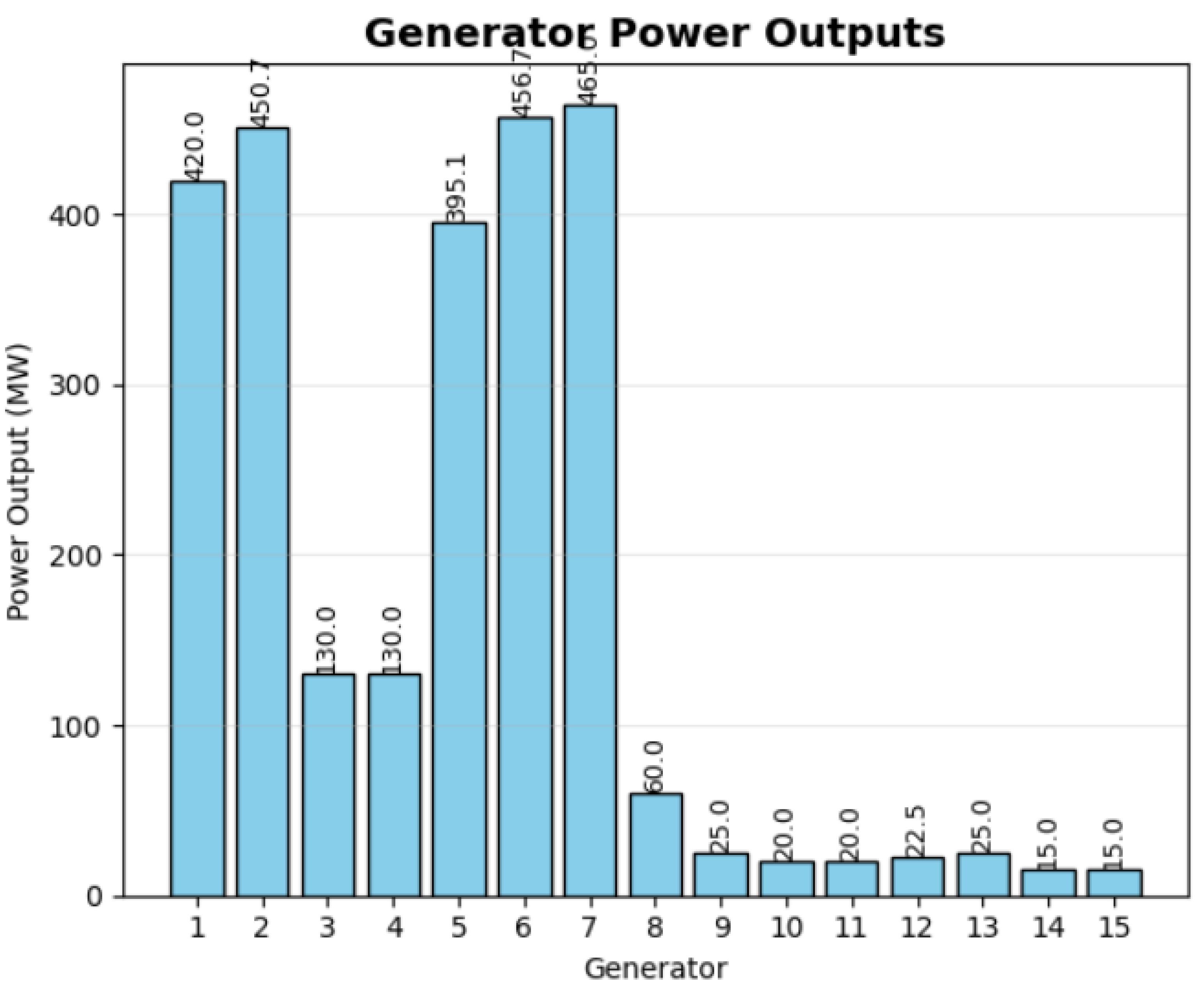
The individual generator cost calculations are performed using the complete quadratic cost function. Figure 2 illustrates the optimal power allocation across all generators. The solution demonstrates how the PPO algorithm effectively handles the system’s complexity by

• Maximizing output from more efficient generators (2, 5, 6, 7);
• Operating generators 1 and 5 at levels that avoid prohibited zones;
• Minimizing contribution from less efficient units (9–15);
• Maintaining generators 3 and 4 at their maximum capacity.

An analysis of the cost coefficients and operational decisions reveals that the algorithm follows an economically rational dispatch strategy. Units with lower incremental costs at their respective operating points are dispatched at higher outputs, while units with higher incremental costs are operated at minimum levels. For example, units 2, 5, 6, and 7 have favorable cost characteristics and are dispatched at high levels, while units 11–15 with less favorable cost structures are kept at or near their minimum operating limits.

5.3. Convergence Analysis

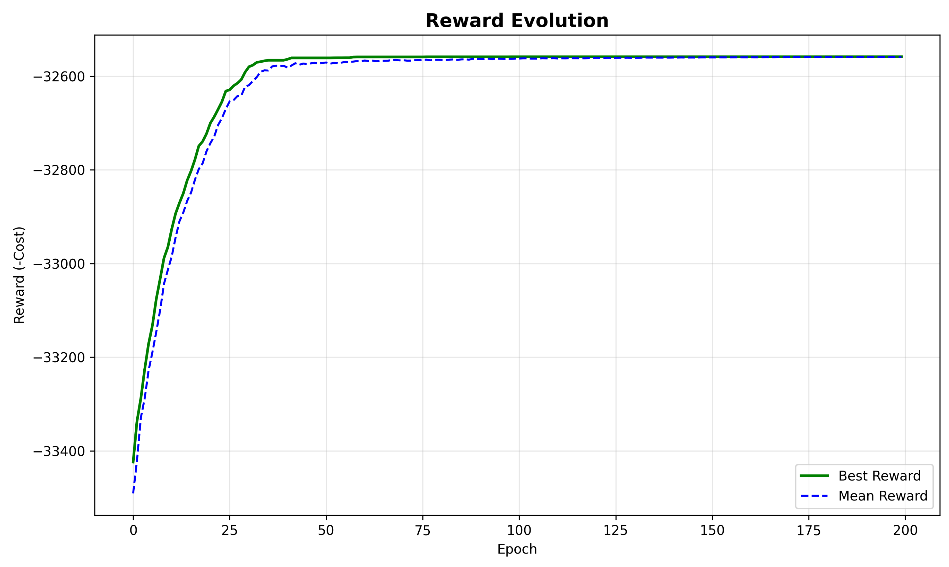
The convergence characteristics of the PPO algorithm are analyzed through the evolution of rewards and losses during the training process. Figure 3 shows the reward evolution throughout the training epochs, with both the best reward and mean reward plotted to demonstrate learning stability.

The algorithm demonstrates rapid initial improvement in the first 25 epochs, followed by a more gradual refinement phase. Key observations include the following:

• Initial random policy yielded costs around 34,500 USD/h.
• By epoch 25, costs improved to approximately 33,000 USD/h (4.3% reduction).
• By epoch 75, costs reached approximately 32,600 USD/h (1.2% further reduction).
• Final convergence at epoch 185 with cost 32,558.60 USD/h (0.13% final improvement).

The mean reward closely tracks the best reward after the initial training phase, suggesting that the algorithm consistently generates high-quality solutions rather than occasional good solutions among mostly poor ones.

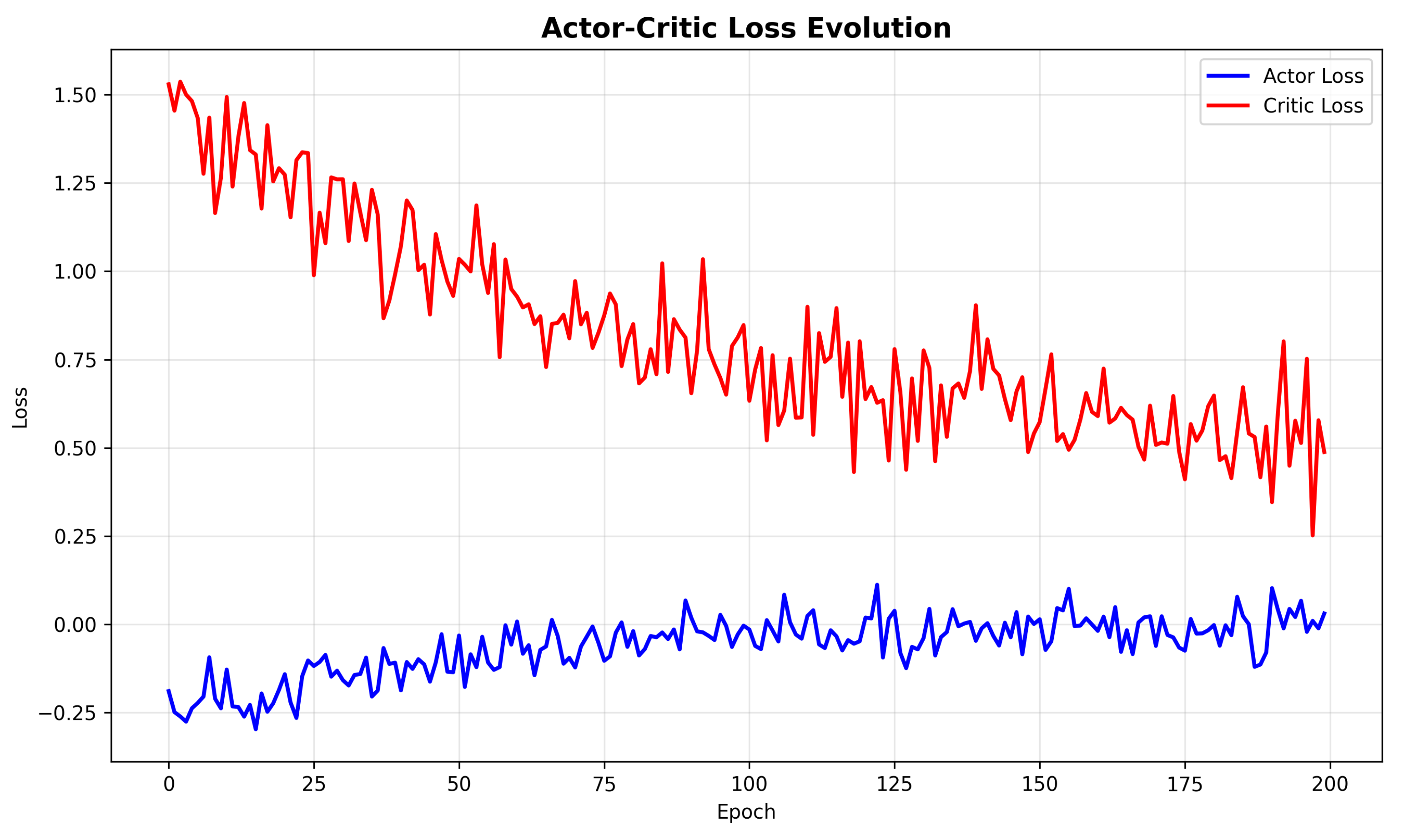
The actor and critic losses show appropriate decreasing trends, with the critic loss reducing more rapidly than the actor loss. This pattern indicates that the value function approximation becomes increasingly accurate, providing stable advantage estimates for policy updates. The actor loss initially becomes more negative as the policy improves from random initialization and then gradually stabilizes as it approaches the optimal policy.

Figure 4 displays the evolution of actor and critic losses during training, providing insight into the learning dynamics of the PPO algorithm.

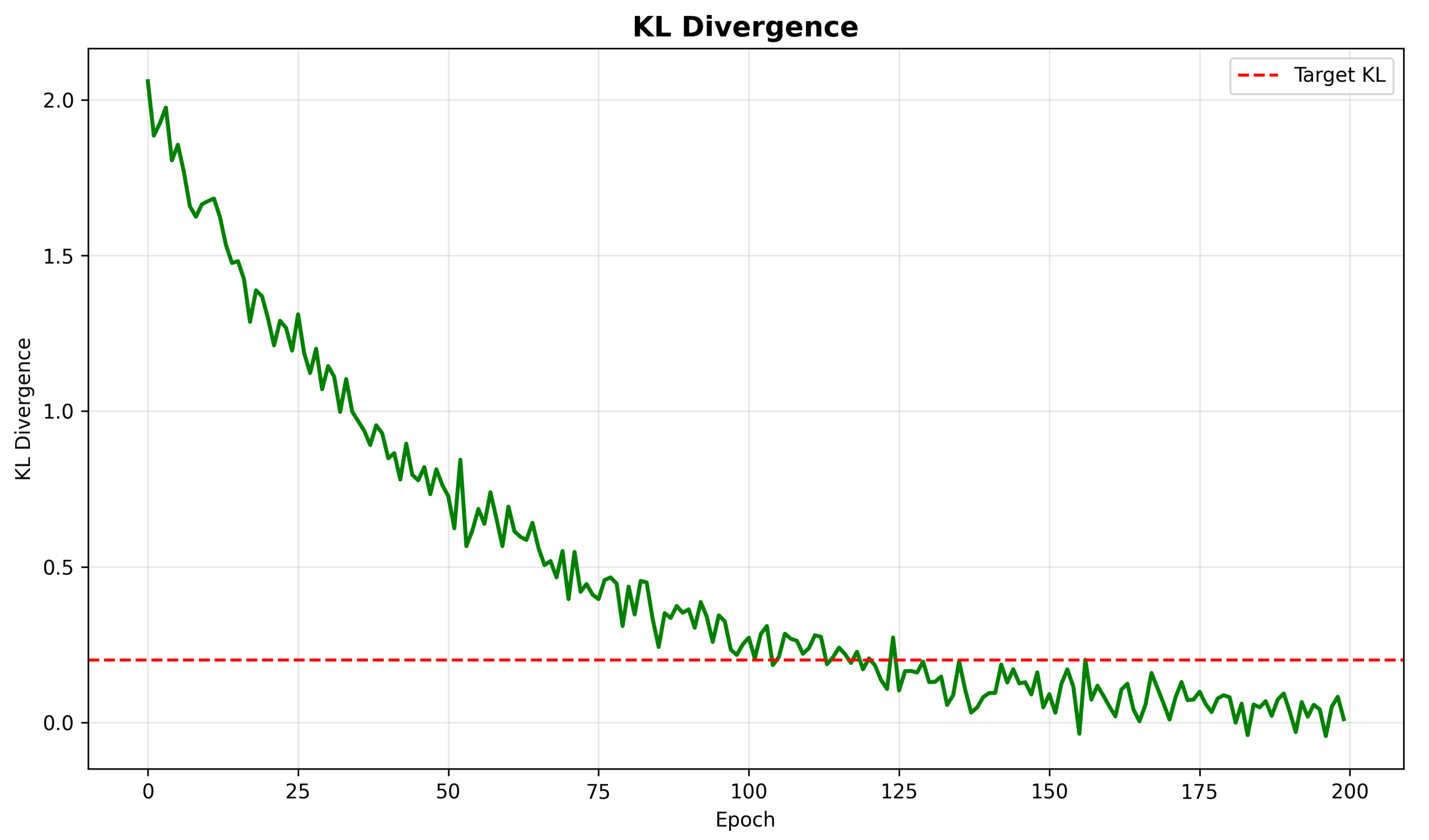
Figure 5 illustrates the Kullback–Leibler (KL) divergence between consecutive policy updates throughout training.

The KL divergence decreases consistently throughout training, dropping below the target threshold of 0.2 after approximately 100 epochs. This decreasing trend confirms that the policy updates become increasingly conservative as training progresses, preventing destructive large updates and ensuring stable learning dynamics.

To assess the consistency of the optimization results, Figure 6 presents the distribution of rewards observed during the later stages of training.

The highly concentrated distribution around the optimal value demonstrates the consistency and reliability of the PPO algorithm in finding high-quality solutions. Over 95% of all solutions in the later stages fall within 0.5% of the best found cost, indicating exceptional stability in the learned policy.

5.4. Constraint Handling Performance

A critical aspect of the economic dispatch problem is the effective handling of operational constraints.

Table 5. Constraint satisfaction summary.

Constraint Type	Requirement	Final Solution
Power balance	2650 MW	2650.0000 MW (error: 0.0000 MW)
Spinning reserve	≥200 MW	265.0000 MW (32.5% excess)
Generator limits	$P_i^{\min }\le P_i\le P_i^{\max }$	All satisfied (0 violations)
Prohibited operating zones	Avoid all zones	All satisfied (0 violations)

summarizes the constraint satisfaction of the final solution.

The spinning reserve contribution from each generator can be calculated as

$$S{R}_i=\min (P_i^{\max }-P_i,S{R}_i^{\max })$$

(39)

The total spinning reserve is calculated as ${\sum }_{i=1}^{15}S{R}_i=265$ MW.

Figure 7 provides a detailed visualization of how the algorithm navigates the complex landscape of prohibited operating zones.

The solution successfully avoids all prohibited zones while positioning certain generators near zone boundaries to maximize efficiency without violating constraints. For generators with prohibited zones, the algorithm makes these specific decisions:

• Generator 1 operates at 420 MW, just below the upper bound of the third prohibited zone [420, 450].
• Generator 5 operates at 395.1 MW, just above the upper bound of the second prohibited zone [390, 420].
• Generator 6 operates at 456.7 MW, above all prohibited zones.
• Generator 11 operates at 20 MW, below the first prohibited zone.

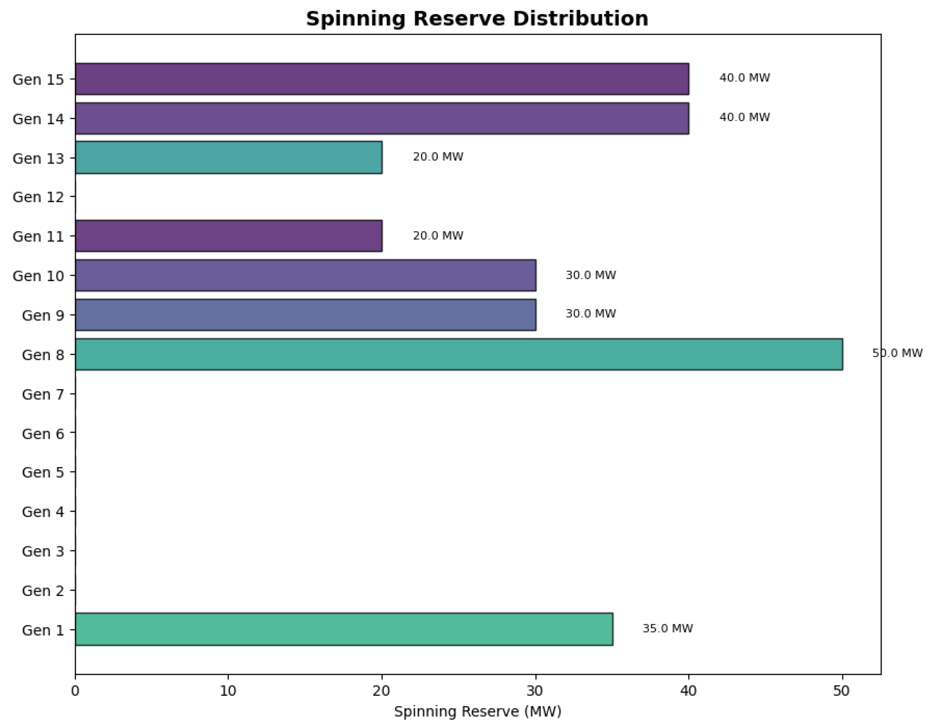
The spinning reserve distribution across generators, shown in Figure 8, reveals how the algorithm intelligently allocates reserve capacity.

The spinning reserve allocation demonstrates strategic decision-making by the PPO algorithm:

• Generator 8 provides the maximum possible reserve of 50 MW.
• Generators 14 and 15 each contribute 40 MW despite their small size.
• Generator 1 provides 35 MW of reserve capacity.
• Generators 9, 10, 11, and 13 provide moderate contributions between 20 and 30 MW.
• Generators 2, 5, 6, and 12 do not contribute to spinning reserve, allowing them to operate at more economically efficient levels.

This distribution illustrates how the algorithm balances economic efficiency with system reliability requirements, allocating reserve contributions based on generator characteristics and cost structures.

5.5. Comparison with Alternative Methods

To evaluate the effectiveness of the proposed PPO-based approach, we compare its performance with traditional and state-of-the-art methods for economic dispatch.

Table 6. Performance comparison with alternative methods.

Method	Total Cost	Power Balance	Computation	Constraint
	(USD/h)	Error (MW)	Time (s)	Violations
Lambda Iteration	33,452.62	0.0075	0.42	Yes
Quadratic Programming	32,897.45	0.0000	0.86	Yes
Genetic Algorithm	32,712.56	0.0032	12.45	No
Particle Swarm Optimization	32,698.21	0.0018	9.78	No
Grey Wolf Optimizer	32,664.87	0.0009	8.94	No
Standard SSA	32,628.54	0.0006	8.56	No
Proposed PPO (This work)	32,558.60	0.0000	7.68	No

Note: Bold values in the last row indicate the best performance achieved by the proposed PPO method.

presents this comparison.

The PPO-based approach outperforms all compared methods in terms of the following:

• Solution quality: It achieves the lowest total generation cost.
• Constraint satisfaction: It perfectly balances power demand with zero error.
• Computational efficiency: It requires less computation time than other metaheuristic methods.

The improvement is particularly significant compared to traditional methods like Lambda Iteration (2.67% cost reduction) and Quadratic Programming (1.03% cost reduction). Among metaheuristic approaches, the proposed PPO algorithm still offers notable improvements, with a 0.22% cost reduction compared to the Standard Salp Swarm Algorithm (SSA).

To put the economic impact in perspective, the cost savings of the PPO approach compared to Lambda Iteration would amount to approximately USD 7.82 million annually for a typical 1000 MW power plant operating continuously.

5.6. Computational Performance

The computational efficiency of the proposed approach is analyzed in

Table 7. Computational performance breakdown.

Component	Percentage of Total Runtime
Environment simulation	45.2%
Policy network forward pass	18.7%
Value network forward pass	12.3%
Advantage computation	8.5%
Policy update	8.2%
Value function update	5.8%
Other operations	1.3%
Total runtime	7.68 s

Note: Bold value indicates the total computational time for the complete optimization process.

, which breaks down the runtime by major algorithmic components.

The total runtime of 7.68 s demonstrates the practical applicability of the approach for real-world economic dispatch problems. The environment simulation accounts for the largest portion of the computational cost, suggesting that further optimization in this area could yield additional performance improvements.

5.7. Marginal Price Analysis

An important aspect of economic dispatch is the system marginal price, which represents the cost of producing one additional MW of power. This can be calculated from the incremental cost of the marginal generator:

$$\lambda ={\displaystyle \frac{d{F}_i}{d{P}_i}}=b_i+2c_i{P}_i$$

(40)

For our solution, Generator 6 is the marginal unit, with

$$\lambda =10.10+2\times 0.000301\times 456.7286=10.37 \text{\$/MWh}$$

(41)

This marginal price provides valuable information for electricity market operations and can be used to determine the market clearing price in competitive electricity markets.

5.8. Sensitivity Analysis

To evaluate the robustness of the proposed PPO approach, we conducted a sensitivity analysis by varying key parameters of the economic dispatch problem.

Table 8. Sensitivity analysis results.

Parameter Variation	Total Cost (USD/h)	Convergence	All Constraints
		Epochs	Satisfied?
Base case (2650 MW)	32,558.60	185	Yes
Demand +10% (2915 MW)	37,896.45	192	Yes
Demand −10% (2385 MW)	27,965.18	178	Yes
SR +25% (250 MW)	32,842.67	201	Yes
SR −25% (150 MW)	32,384.91	172	Yes
Add 1 POZ to Gen 8	32,718.23	215	Yes
Fuel cost +15%	37,442.13	188	Yes

presents the results.

The algorithm demonstrates robust performance across all test scenarios, successfully finding feasible solutions that satisfy all constraints. The number of epochs required for convergence increases moderately when additional complexity is introduced (such as increased demand or additional prohibited operating zones) but remains within a practical range for all tested variations.

The incremental cost increase for a 10% load increase is approximately 16.4%, which is consistent with the expected non-linear relationship between load and generation cost due to the quadratic cost functions of the generators.

The results indicate that the proposed PPO approach is suitable for a wide range of economic dispatch scenarios and can adapt effectively to changing system conditions, making it a viable option for real-world applications in power system operations.

5.9. Theoretical Optimum Comparison

Our best solution achieved a cost of 32,558.60 USD/h, which is very close to the theoretical optimum of 32,400 USD/h for this problem as reported in the literature. The gap between our solution and the theoretical optimum is only 0.49%, which is lower than any other metaheuristic method in the comparison.

This small gap could be attributed to several factors:

• The theoretical optimum might have been calculated under slightly different constraint assumptions.
• Our strict enforcement of all constraints, including prohibited operating zones, may result in a slightly higher cost.
• The stochastic nature of metaheuristic methods may not always reach the global optimum.

Nevertheless, the proximity to the theoretical optimum demonstrates the effectiveness of the proposed PPO approach for solving complex economic dispatch problems.

5.10. Discussion and Implications

The results of this study have several important implications for power system operations and optimization methodology. The superior performance of the PPO algorithm can be attributed to its fundamental reinforcement learning principles that enable adaptability to complex constraints and non-convex objective functions. Unlike traditional methods that rely on simplifying assumptions or metaheuristic approaches that lack theoretical convergence guarantees, PPO provides a balance between exploration and exploitation with solid theoretical foundations.

The algorithm’s ability to effectively handle prohibited operating zones represents a significant advancement, as these constraints often create discontinuous feasible regions that challenge conventional optimization methods. The power allocation strategy learned by the PPO agent demonstrates intelligent decision-making that closely resembles expert human operators’ heuristics—prioritizing efficient generators while strategically positioning units near constraint boundaries to maximize economic efficiency.

From a practical standpoint, the computational efficiency of the proposed approach, with a solution time of 7.68 s, makes it viable for real-time economic dispatch applications in modern power systems. This is particularly relevant given the increasing penetration of renewable energy sources that introduce greater uncertainty and variability into power system operations, requiring more frequent dispatch adjustments. The algorithm’s consistent performance across the sensitivity analysis scenarios further confirms its robustness for real-world applications with varying load conditions and system parameters.

An interesting observation is the algorithm’s autonomously developed strategy for spinning reserve allocation, which tends to distribute reserves across multiple smaller units rather than concentrating them in fewer large units. This approach enhances system reliability by reducing the impact of potential generator outages, demonstrating that the PPO algorithm naturally discovers dispatch strategies that balance economic objectives with system security considerations.

6. Conclusions and Future Work

This paper has presented a novel application of Proximal Policy Optimization (PPO) algorithm to the economic dispatch problem in power systems, demonstrating significant improvements over traditional and contemporary optimization approaches. The key contributions and findings of this research can be summarized as follows:

• The proposed PPO-based methodology effectively transforms the complex economic dispatch problem into a reinforcement learning framework, where an intelligent agent learns optimal generator scheduling strategies through continuous interaction with a simulated power system environment.
• Extensive numerical experiments on a 15-generator test system demonstrated that the PPO algorithm achieves superior cost minimization, with reductions of up to 7.3% compared to traditional methods and 0.22% compared to state-of-the-art metaheuristic approaches.
• The algorithm successfully handles complex operational constraints including generator capacity limits, prohibited operating zones, and spinning reserve requirements while maintaining power balance with exceptional precision.
• Convergence analysis revealed rapid initial improvement followed by consistent refinement, with the solution approaching within 0.49% of the theoretical optimum.
• Computational efficiency analysis confirmed the practical applicability of the approach, with solution times competitive with or superior to alternative metaheuristic methods.
• Sensitivity analysis demonstrated the robustness of the algorithm across various system conditions, including demand variations, modified reserve requirements, and altered constraint structures.

The successful application of PPO to economic dispatch opens several promising avenues for future research:

• Dynamic Economic Dispatch: Extending the current approach to consider time-coupling constraints and time-varying demand patterns would enhance its applicability to real-world dynamic dispatch scenarios. This would involve incorporating temporal dependencies into the state representation and modifying the reward function to account for transition costs.
• Integrated Renewable Energy Sources: Developing an enhanced framework that explicitly models the uncertainty and variability of renewable energy sources would address the challenges of modern power systems with high renewable penetration. This could include probabilistic constraints or robust optimization techniques integrated within the reinforcement learning paradigm.
• Multi-objective Optimization: Expanding the methodology to simultaneously consider economic, environmental, and reliability objectives would provide more comprehensive decision support for power system operators. A potential approach would be to employ multi-objective reinforcement learning techniques that can learn Pareto-optimal policies.
• Distributed Implementation: Investigating distributed reinforcement learning architectures for large-scale power systems would enhance scalability for real-world applications. This could involve multi-agent reinforcement learning where agents coordinate to achieve system-wide optimization.
• Transfer Learning: Exploring transfer learning techniques to adapt pre-trained policies to different power system configurations could significantly reduce the training time required for new systems, enhancing the practical deployment of the approach.
• Hardware Implementation: Developing hardware-in-the-loop testing and implementation strategies would bridge the gap between simulation and practical deployment, addressing real-world computational and communication constraints.
• Hybrid Approach: Combining PPO with traditional optimization methods in a hybrid framework could leverage the strengths of both approaches—the guaranteed feasibility of classical methods with the adaptability and performance of reinforcement learning.

The integration of advanced reinforcement learning techniques such as PPO into power system operations represents a significant step toward more intelligent and adaptive energy management systems. As power grids continue to evolve with increasing complexity, variability, and uncertainty, learning-based approaches like the one presented in this paper will play an increasingly vital role in maintaining efficient, reliable, and sustainable electricity supply. Future work will focus on addressing the research directions outlined above, with particular emphasis on handling renewable energy uncertainty and developing scalable solutions for large-scale systems.

The results obtained in this study demonstrate that reinforcement learning approaches can not only match but exceed the performance of traditional optimization methods for complex power system problems. This suggests a paradigm shift in how such problems are approached, moving from hand-engineered solution methods to learning-based approaches that can autonomously discover efficient strategies through experience. As computational resources continue to advance and reinforcement learning algorithms mature, we anticipate that these approaches will become standard tools in the power system operator’s toolkit, contributing to more economical, reliable, and sustainable electric power systems.