Abstract
Second-order Linear Active Disturbance Rejection Controller (SLADRC) is a powerful control technique. Ongoing research is focused on simplifying tuning procedures, extending applicability to handle more complex systems, and ensuring efficient real-time implementation. In this proposed work, four different tuning approaches, using the Atomic Orbital Search (AOS) optimization algorithm concerning the number of tuning parameters, are presented. The performance of each tuning method for stabilizing the rotary inverted pendulum in the upright position and tracking trajectory is analyzed and validated through simulation and experimentation. The results indicate that the reduced number of SLADRC controller parameters tuned using AOS optimization provides superior performance compared to the controller with more tuning parameters for the nonlinear rotary inverted pendulum. From the analysis method, II tuning, provide the optimum results of settling time (), 1.5 s, and maximum angle deviation of .
1. Introduction
The rotary inverted pendulum (RIP) is a key challenge in control theory and robotics, often used as a model for real-world applications like space booster attitude control, automatic landing of aerial vehicles, aircraft stabilization, humanoid robots, and crane systems. It is inherently nonlinear and underactuated, and its open-loop unstable dynamics make control difficult. Various control methods, such as 2DOF PID [1], FOPID [1,2], SMC [3], LQR [4], and feedback linearization, have been explored in the literature, all of which demand precise system knowledge and tuning for optimal performance. This study focuses on Active Disturbance Rejection Control (ADRC) [5,6,7,8], a modern, model-free controller known for its fast disturbance rejection. Many real-world systems exhibit nonlinear behavior that can complicate the design and performance of ADRC. Effective methods to handle nonlinearities within the ADRC framework are still being researched. Linear ADRC (LADRC) [9], introduced by Gao, simplifies tuning and is widely applicable. First-order LADRC uses a second-order Extended State Observer (ESO) but faces challenges with complex systems, while second-order LADRC (SLADRC) incorporates a third-order ESO and a PD controller, which are better suited for managing system nonlinearities. SLADRC tuning typically employs bandwidth parameterization. Increasing the order of LADRC complicates the selection of controller dynamics and provides similar performance as lower-order LADRC.
This research investigates SLADRC parameter selection for balancing and trajectory tracking of RIP using various tuning approximations and methods followed in the literature. In general, system performance varies based on the number of tuning parameters involved. The Atomic Orbital Search (AOS) [10] algorithm is applied efficiently to determine the optimal tuning parameters [11] for each approximation.
2. Problem Description
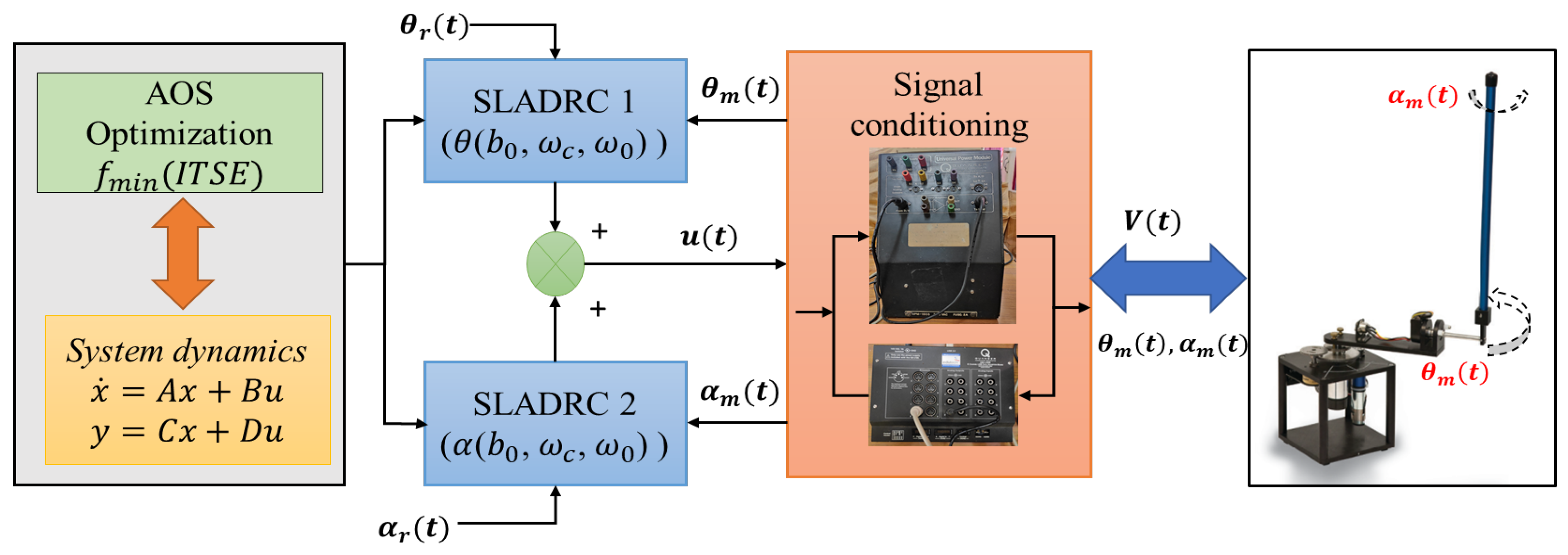
Design of distinct SLADRC controllers for stabilizing the pendulum angle () at the equilibrium point and trajectory tracking of the motor angle () using DC servo motor with input voltage (V) of the range ±5 V. For tuning the controller parameters, the AOS technique is utilized with the linear model of the RIP. The overall schematic is shown in Figure 1.
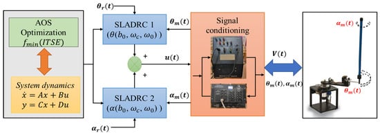
Figure 1.
Schematic of proposed tuning for the RIP.
2.1. Mathematical Modeling of the RIP
The Linearized dynamic equations of motion of RIP [12] are,
The parameter values of RIP in Equations (1) and (2). The obtained state space equation of the model of the system is
The transfer function for change in motor angle () and change in pendulum angle (), with respect to change in motor voltage () obtained from Equation (3), is given below:
2.2. SLADRC Preliminaries
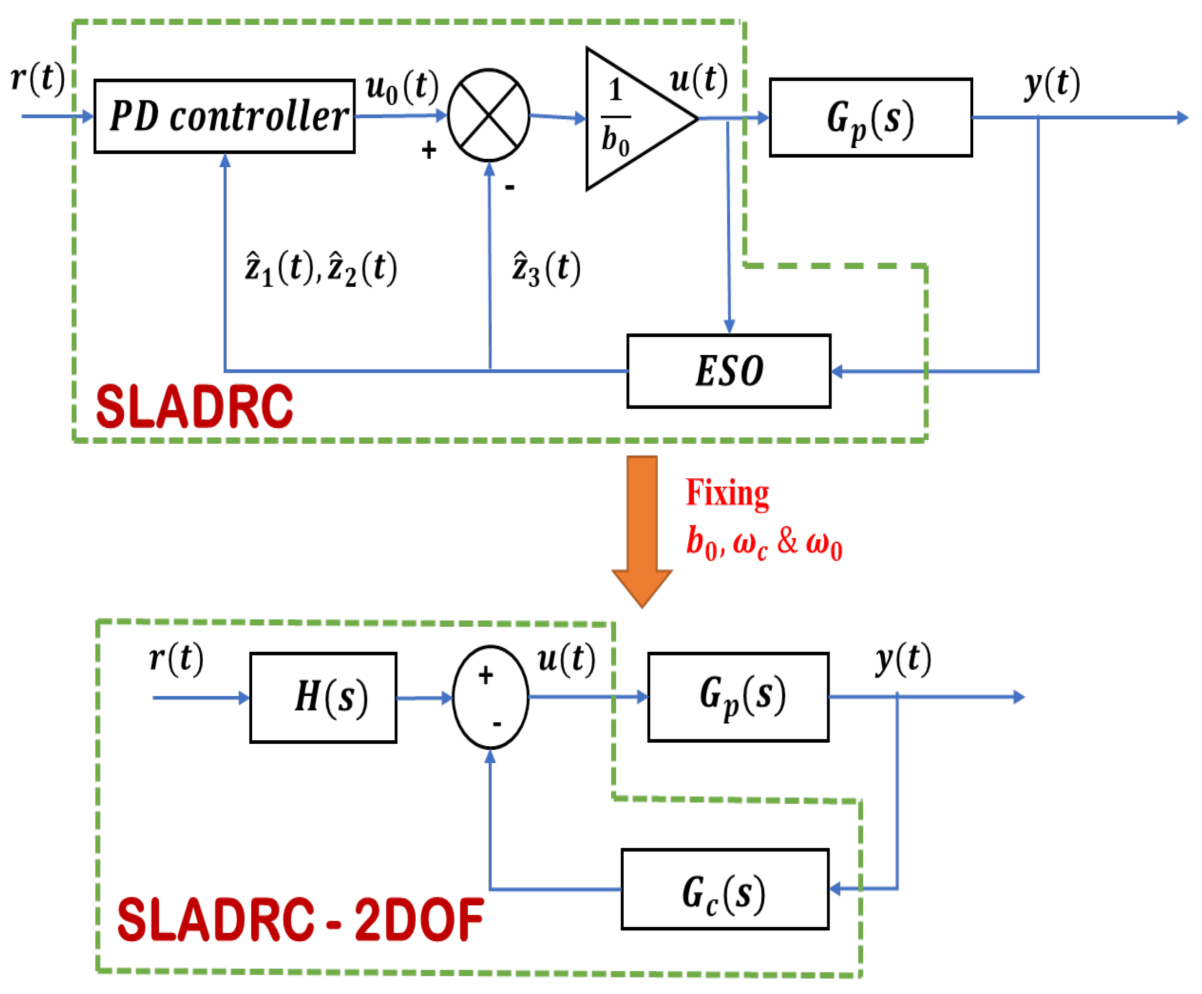
Figure 2 illustrates the generalized SLADRC structure, which consists of two parts: an ESO and a feedback controller.
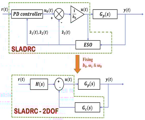
Figure 2.
SLADRC structures.
The ESO estimates both the states and the total disturbance () at the same time. The feedback controller that cancels the total disturbance and achieves the desired performance.
The control law of SLADRC is defined as
where and are the controller gains, is the reference signal, are the states of the system, and are the estimates of and .
The second-order ESO structure obtained from the literature is
According to the bandwidth parameterization technique, the observer and controller poles are located at and , respectively, where is the observer bandwidth and is the controller bandwidth. Now there are only three tuning parameters . The depends on the (i.e., .
where is the multiplication factor. Transfer function form of the equations is obtained by substituting the controller and observer gains and the Laplace transform of Equation (7) in Equation (6). This gives the 2-DOF SLADRC structure, in terms of feedforward transfer function and feedback transfer function , as
Equations (9) and (10) show the compact 2 DOF structure of SLADRC with limited parameters. In the literature, various versions of approximating the tuning parameters for reducing the complexity in the design of SLADRC are discussed. From this, four major methods of approximating the parameters are taken for analyzing the performance of the RIP, as shown in Table 1.

Table 1.
Classification of tuning methods.
3. Atomic Orbital Search Optimization
The Atomic Orbital Search (AOS) algorithm is a recent and successful metaheuristic optimization technique that effectively explores the search space to find global or near-optimal solutions for complex problems. In atomic orbitals, electrons organize themselves to achieve minimal atomic energy. Similarly, the AOS optimization algorithm structures its population in search space to minimize the objective function. Known for its fast and adaptable performance, AOS can handle a wide range of systems, including linear, nonlinear, constrained, and multimodal problems. AOS provides a flexible and efficient method for selecting control parameters for different applications.
The initial population of electrons () represents the various tuning parameters utilized by different methods. The objective function of the algorithm is to obtain the lowest energy levels from the large set of energy values () derived from the population. Based on the values of Binding State () and Binding Energy (), the position of the electron is updated to the next imaginary layer at each iteration. The new position update equation is given as
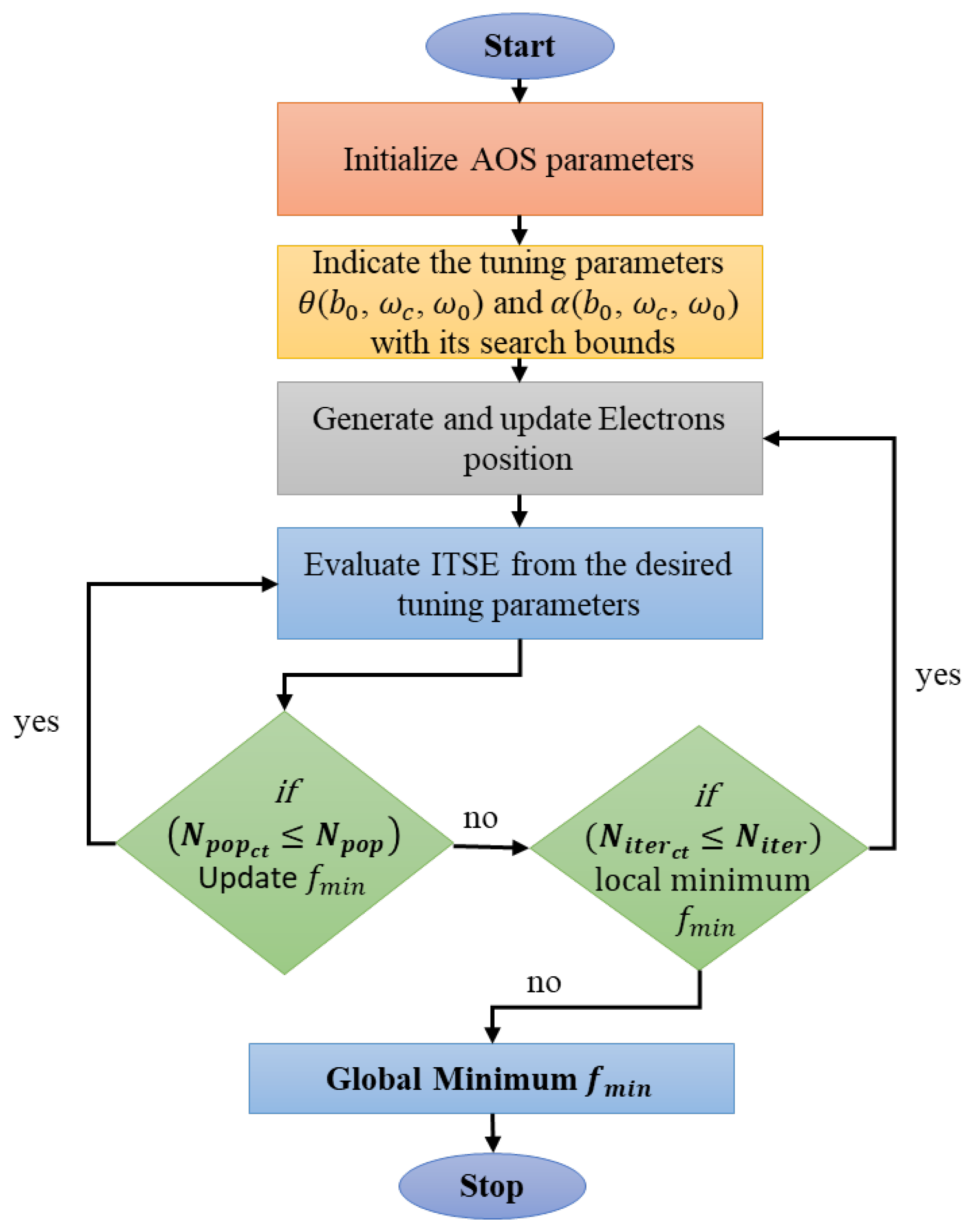
where , , and are uniform random values ranging between 0 and 1. is the lowest energy value at each iteration. The AOS framework for implementation is shown in Figure 3.

Figure 3.
AOS framework.
In this research work, AOS is used to optimize the parameters of a SLADRC controller to control the position of underactuated rotary inverted pendulum, where it simulates the behavior of electrons to find the optimal values of the controller parameters that minimize a cost function. The cost function is formulated by minimizing the deviation between the desired and actual values of settling time and peak overshoot to ensure the desired transient performance and robustness. The six key controller parameters for the motor angle and for the pendulum angle are chosen as AOS parameters and their corresponding search boundaries are provided in Table 2.
Table 2.
RIP system and controller parameter values.
The objective function is designed by summing the ITSE minimization terms for both the motor angle and the pendulum angle, ensuring an improved transient response with a faster settling time, minimal overshoot, and a balanced control effort, as given below.
where is the motor angle deviation, is the pendulum angle deviation, and represents the simulation time.
Remark 1:
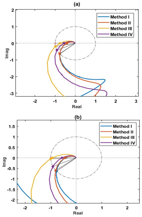
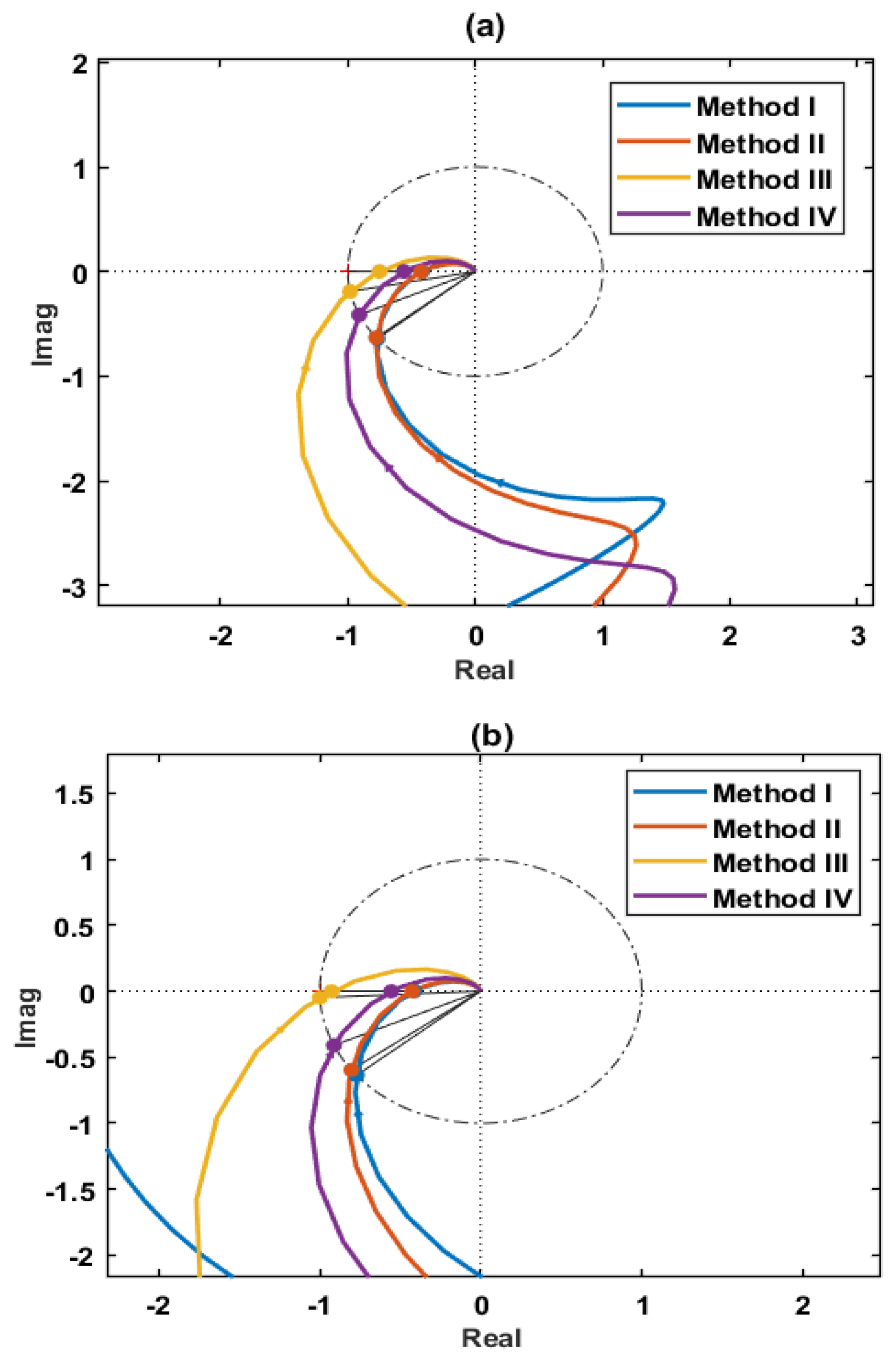
The stability of the closed-loop system is analyzed using the Nyquist stability criterion for the linearized RIP model, as presented in Equations (4) and (5). The designed controllers are represented as and . The closed-loop characteristic equation of the RIP system is expressed as . The corresponding loop transfer function is given as .Figure 4 validates the stability and robustness of each system for the controllers designed based on different approximation methods.
Figure 4.
Nyquist plots of plant transfer function with controllers (a) and (b) .
4. Results and Discussion
To determine the optimal tuning parameters for each method, the AOS optimization technique was applied using a linearized model of the pendulum with initial state values ([θ, α, , ] = [1⁰, 0.1⁰, 0, 0]) to improve model accuracy. The optimal parameters, along with their angle variations, fitness values, and computation time, are shown in Table 3. Table 4 provides a simulation and experimental comparison of each tuning method. As shown in Figure 5a, all methods achieve good stability and performance in tracking and disturbance rejection. However, Method I exhibits significant oscillation in simulation due to poor tuning and boundary region selection. Figure 4a,b shows the Nyquist plots of the loop transfer functions with different controllers. In Method II, the k value ranges between 8 and 12; beyond this, the observer bandwidth increases, leading to instability. In Methods III and IV, k is fixed, allowing flexibility in tuning and (in terms of and for Method IV) to achieve optimal performance.
Table 3.
SLADRC optimized parameter values for different tuning methods.
Table 4.
Simulation and Experimental comparison of various tuning methods in SLADRC.
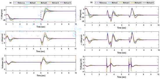
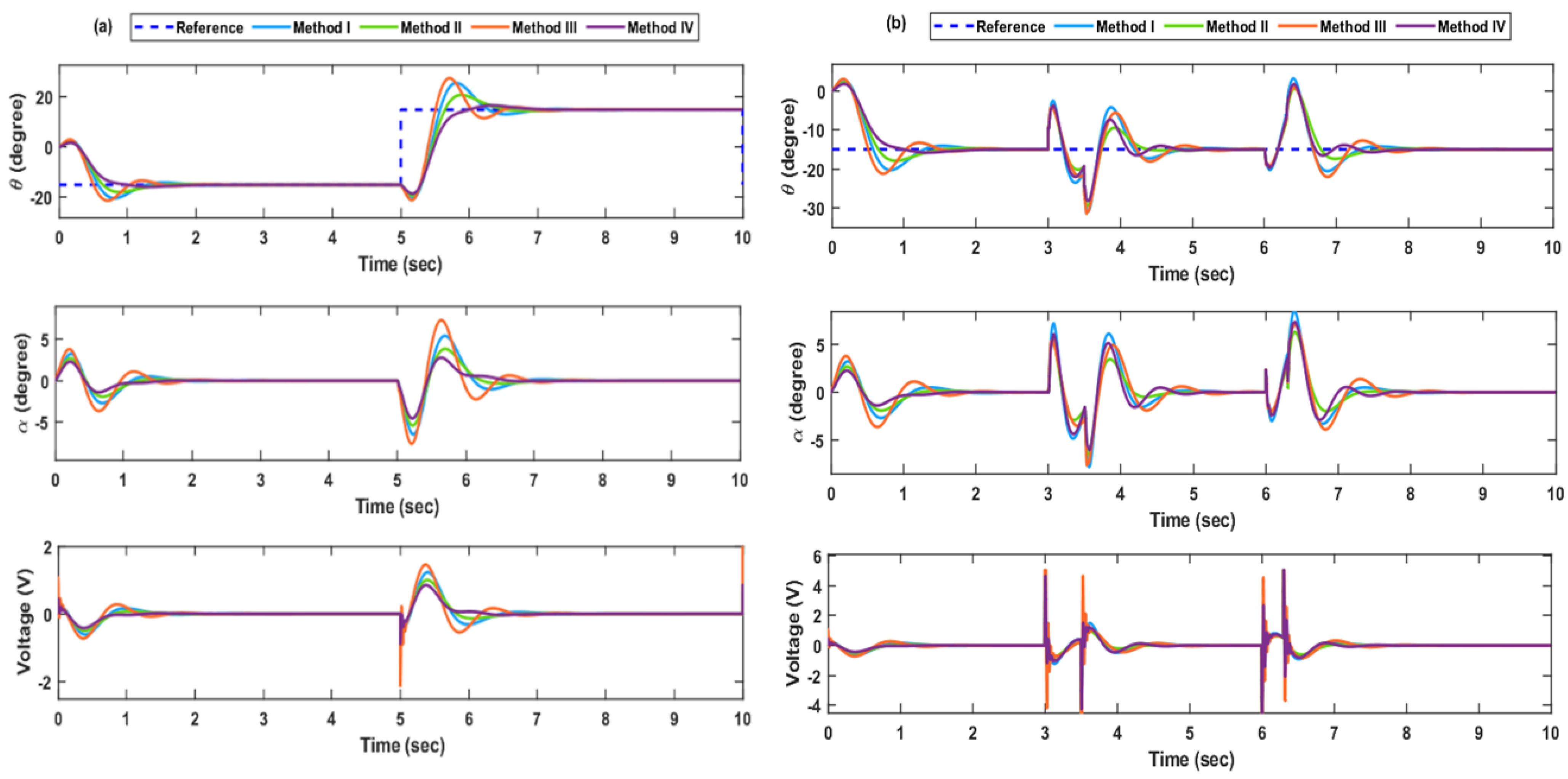
Figure 5.
(a) Set point tracking of motor angular position and pendulum angle in simulation, (b) regulatory response of motor and pendulum angle in simulation.
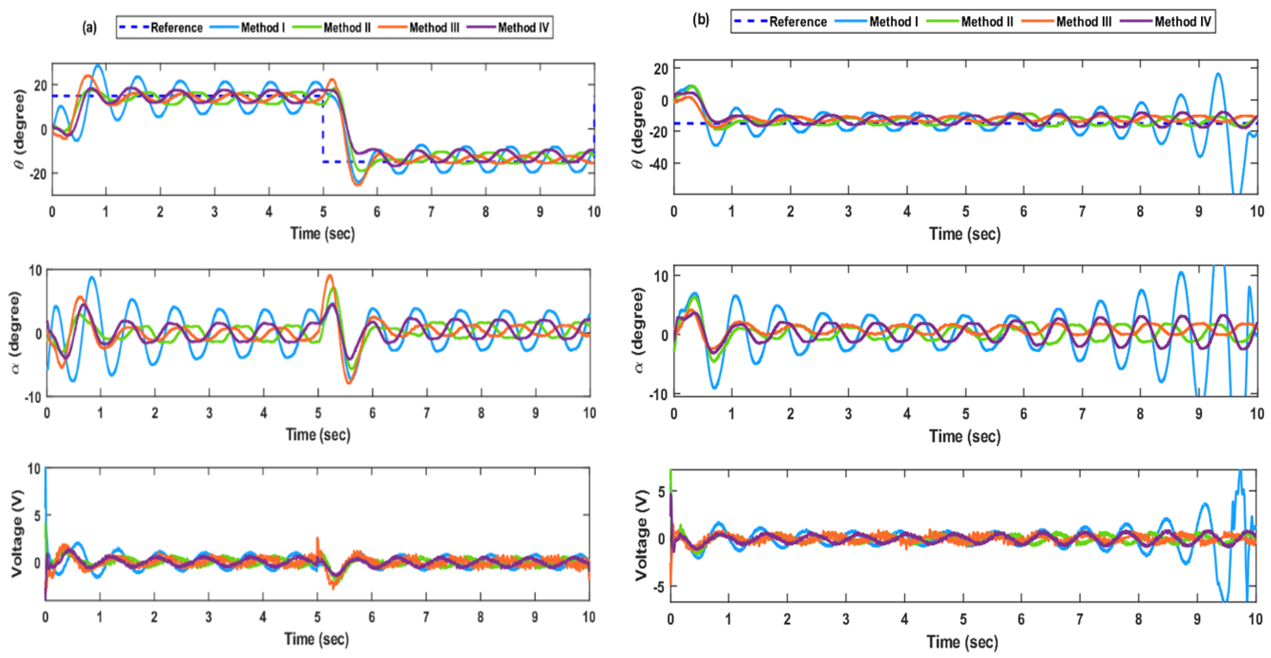
To assess disturbance rejection, a disturbance of 1⁰ is added at 3–3.5 s for the motor angle (θ) and 0.1⁰ at 5–5.2 s for the pendulum angle (α), as shown in Figure 5b. In the experiments, robustness is tested by adding a 10 g tip mass from 5 to 10 s, as shown in Figure 6b. Figure 6a,b demonstrates the servo and regulatory results for RIP, showing that Methods II, III, and IV have better performance with smaller oscillations in tracking. Method I shows large oscillations in the servo response and becomes unstable under parameter uncertainty, as shown in Figure 6b. This study confirms that increasing the number of tuning parameters complicates design and hinders optimal performance, while better results are achieved with fewer tuning parameters, as confirmed by the ITSE values in Table 4. The k value must be optimal. Methods II and III demonstrate strong disturbance rejection, with Method III showing the least angle deviation and optimal results, as shown in Table 3 and Table 4.
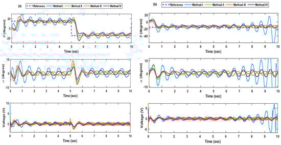
Figure 6.
(a) Set point tracking of motor angular position and pendulum angle in real time; (b) regulatory response of motor and pendulum angle in real time.
5. Conclusions
The performance and robustness of four different tuning techniques of SLADRC are discussed for the unstable RIP. From the results, it is clear that increasing the controller parameter reduces the performance and robustness due to the inability to select optimum values. Increasing the multiplication factor ‘k’ value larger than 10 increases phase lag in the loop and reduces robustness of the system. The choice of k value as 10 provides better estimation of parameters and time domain performance for most of the LTI systems and it violates complex nonlinear systems. From the overall analysis, it is clear that the fixing controller, observer bandwidth, and k (Method II and III) provide better performance and robustness for the RIP and other complex systems.
Author Contributions
Conceptualization, methodology, validation, experimentation, investigation, and writing—J.G. Supervision, review, editing, visualization, and project administration—E.D. All authors have read and agreed to the published version of the manuscript.
Funding
This research received no external funding.
Institutional Review Board Statement
Not applicable.
Informed Consent Statement
Not applicable.
Data Availability Statement
Data will be available upon request.
Conflicts of Interest
The authors declare no conflicts of interest.
References
- Adharsh Lal, M.; Kunjumuhammed, A.; Tomy, J.; Urmila, G.; Sivadas, M.; Mohan, A. Stabilization of Rotary Inverted Pendulum using PID Controller. In Proceedings of the 2021 8th International Conference on Smart Computing and Communications: Artificial Intelligence, AI Driven Applications for a Smart World, ICSCC 2021, Kochi, India, 1–3 July 2021; Institute of Electrical and Electronics Engineers Inc.: Piscataway, NJ, USA, 2021; pp. 376–380. [Google Scholar]
- Dwivedi, P.; Pandey, S.; Junghare, A.S. Robust and novel two degree of freedom fractional controller based on two-loop topology for inverted pendulum. ISA Trans. 2018, 75, 189–206. [Google Scholar] [CrossRef] [PubMed]
- Nagarajan, A.; Victoire, A.A. Optimization Reinforced PID-Sliding Mode Controller for Rotary Inverted Pendulum. IEEE Access 2023, 11, 24420–24430. [Google Scholar] [CrossRef]
- Fatihu Hamza, M.; Jen Yap, H.; Ahmed Choudhury, I. Cuckoo search algorithm based design of interval Type-2 Fuzzy PID Controller for Furuta pendulum system. Eng. Appl. Artif. Intell. 2017, 62, 134–151. [Google Scholar] [CrossRef]
- Pan, J.; Qi, S.; Wang, Y. Flatness based active disturbance rejection control for cart inverted pendulum and experimental study. In Proceedings of the American Control Conference, Chicago, IL, USA, 1–3 July 2015; Institute of Electrical and Electronics Engineers Inc.: Piscataway, NJ, USA, 2015; pp. 4868–4873. [Google Scholar]
- Ramírez-Neria, M.; Sira-Ramírez, H.; Garrido-Moctezuma, R.; Luviano-Juarez, A. On the linear active disturbance rejection control of the Furuta pendulum. In Proceedings of the American Control Conference, Portland, OR, USA, 4–6 June 2014; Institute of Electrical and Electronics Engineers Inc.: Piscataway, NJ, USA, 2014; pp. 317–322. [Google Scholar]
- Liu, B.; Hong, J.; Wang, L. Linear inverted pendulum control based on improved ADRC. In Systems Science and Control Engineering; Taylor and Francis Ltd.: Abingdon, UK, 2019; Volume 7, pp. 1–12. [Google Scholar]
- Chen, Q.; Zhuang, J.; Liu, B.; Yang, P. Inverted Pendulum Balance Control Based on Improved Active Disturbance Rejection Control. In Proceedings of the 2022 Chinese Automation Congress, CAC 2022, Xiamen, China, 25–27 November 2022; Institute of Electrical and Electronics Engineers Inc.: Piscataway, NJ, USA, 2022; pp. 1526–1531. [Google Scholar]
- Herbst, G. A simulative study on active disturbance rejection control (ADRC) as a control tool for practitioners. Electronics 2013, 2, 246–279. [Google Scholar] [CrossRef]
- Azizi, M. Atomic orbital search: A novel metaheuristic algorithm. Appl. Math. Model. 2021, 93, 657–683. [Google Scholar] [CrossRef]
- Kumar, R.; Bothara, Y.; Ezhilarasi, D.; Mohanavelu, K. Atomic Orbital Search Optimization Based Fractional Order PID Controller for 4 DoF Lower Limb Exoskeleton. In Proceedings of the 2023 International Conference on Power, Instrumentation, Control and Computing, PICC 2023, Thrissur, India, 19–21 April 2023; Institute of Electrical and Electronics Engineers Inc.: Piscataway, NJ, USA, 2023. [Google Scholar]
- Quanser, Rotary Inverted Pendulum Manual. Available online: https://www.made-for-science.com/de/quanser/?df=made-for-science-quanser-rotary-double-inverted-pendulum-coursewarestud-matlab.pdf (accessed on 1 September 2024).
- Hao, Z.; Yang, Y.; Gong, Y.; Hao, Z.; Zhang, C.; Song, H.; Zhang, J. Linear/Nonlinear Active Disturbance Rejection Switching Control for Permanent Magnet Synchronous Motors. IEEE Trans. Power Electron. 2021, 36, 9334–9347. [Google Scholar] [CrossRef]
- Dai, X.; Zhao, C.; Xu, R. Nonlinear Active Disturbance Rejection Control for Vehicle Active Suspension System. In Proceedings of the 2023 3rd International Conference on Electronic Information Engineering and Computer Science, EIECS 2023, Changchun, China, 22–24 September 2023; Institute of Electrical and Electronics Engineers Inc.: Piscataway, NJ, USA, 2023; pp. 633–637. [Google Scholar]
- Wang, Y.; Tan, W.; Cui, W.; Han, W.; Guo, Q. Linear active disturbance rejection control for oscillatory systems with large time-delays. J. Franklin Inst. 2021, 358, 6240–6260. [Google Scholar] [CrossRef]
Disclaimer/Publisher’s Note: The statements, opinions and data contained in all publications are solely those of the individual author(s) and contributor(s) and not of MDPI and/or the editor(s). MDPI and/or the editor(s) disclaim responsibility for any injury to people or property resulting from any ideas, methods, instructions or products referred to in the content. |
© 2025 by the authors. Licensee MDPI, Basel, Switzerland. This article is an open access article distributed under the terms and conditions of the Creative Commons Attribution (CC BY) license (https://creativecommons.org/licenses/by/4.0/).