Integrated Improved Complete Ensemble Empirical Mode Decomposition and Continuous Wavelet Transform Approach for Enhanced Bearing Fault Diagnosis in Noisy Environments ^†

Abstract

Bearings are vital apparatuses in many industrial systems, and their failure can lead to severe damage, costly downtime, and safety risks. Therefore, early detection of bearing faults is critical to prevent catastrophic failures. However, diagnosing bearing faults in real-world conditions is challenging due to noise, which can obscure vibration signals and reduce the effectiveness of traditional diagnostic techniques. This paper portrays a unique method for bearing fault identification in high-noise environments by integrating Improved Complete Ensemble Empirical Mode Decomposition (ICEEMD) and Continuous Wavelet Transform (CWT). ICEEMD decomposes complex vibration signals into intrinsic mode functions, effectively filtering out noise and enhancing feature extraction. CWT is then applied to obtain a time–frequency representation of the cleaned signal, allowing for precise detection of transient events and frequency variations associated with faults. The proposed approach is evaluated using simulated signals, achieving a testing accuracy of 78% at −20 dB SNR, demonstrating its robustness in noisy environments. This study highlights the capability of combining ICEEMD and CWT for robust fault diagnosis in noisy industrial applications, paving the way for improved predictive maintenance strategies.

1. Introduction

Bearings are critical components in various industrial applications, and their failure can lead to severe system damage, costly downtime, and potential safety hazards [1]. Hence, detecting bearing faults early is essential to prevent catastrophic failures. However, diagnosing bearing faults in real-world conditions is challenging due to the presence of noise, which can mask the vibration signals generated by the bearing [2]. Noise arises from various sources, such as mechanical components, environmental conditions, or external disturbances, and it can significantly reduce the accuracy of traditional diagnostic techniques. Therefore, robust methodologies that can effectively separate useful fault information from noise are required.

One such approach is using Empirical Mode Decomposition (EMD)-based techniques, notably ICEEMD. EMD is a signal-processing technique that decomposes non-linear and non-stationary signals into intrinsic mode functions (IMFs), representing oscillatory modes embedded in the signal [3]. However, EMD is affected by mode mixing. To address this, a Complete Ensemble EMD (CEEMD) was proposed [4]. Although CEEMD reduces mode mixing compared to EMD, it does not completely eliminate it. To further mitigate this issue, CEEMD with Adaptive Noise (CEEMDAN) was introduced [5]. However, CEEMDAN remains computationally expensive and retains residual noise. An improved version, ICEEMD, was developed to handle noise more effectively and enhance decomposition quality [6]. This method can effectively decompose complex vibration signals into multiple components, allowing the isolation of useful fault-related features from noise. Ordonez-Bolanos et al. [7] used ICEEMD for the identification of facial emotions.

In addition to decomposing the signal and removing noise, it is crucial to transform the cleaned signal into a representation that facilitates fault detection. Time–frequency analysis (TFA) is a crucial tool for this purpose [8]. In TFA, both time and frequency domain information are preserved, enhancing fault identification efficiency [9]. Cohen’s class of transforms [10] and wavelet transforms [11] are the two major categories used in TFA. The Continuous Wavelet Transform (CWT) has emerged as a compelling tool in recent years, as it provides a time–frequency (TF) representation of the signal, enabling the detection of transient events and frequency variations associated with faults [12]. However, combining the effectiveness of TFA with ICCEMD can further boost the accuracy of bearing fault detection in boisterous environments.

The development of deep learning algorithms has advanced bearing fault diagnosis to the next level. X. Li et al. [13] utilized an adaptive convergent viewable neural network, while C. Liang et al. [14] employed attention-augmented separable residual networks. M. Ye et al. [15] proposed a residual convolutional fusion network. However, these deep learning algorithms are computationally expensive. Effective feature extraction can significantly reduce computational complexity while still leveraging the benefits of machine learning.

While ICEEMD has improved the decomposition quality and noise handling, its effectiveness in highly noisy environments requires further improvement. TFA techniques, such as CWT, provide valuable TF representations of signals. However, the combination of CWT with ICCEMD remains unexplored. While deep learning models have significantly improved fault classification accuracy, they are computationally expensive and require large datasets. Proper feature extraction from CWT combined with ICCEMD could reduce the reliance on deep learning models while still achieving high diagnostic accuracy.

This study aims to develop and implement ICCEMD to improve the decomposition of noisy vibration signals, integrate CWT with ICCEMD for enhanced feature extraction and fault identification, and extract meaningful features from CWT-based representations to reduce computational complexity while maintaining a high fault detection accuracy.

2. Signal Simulation Model

Initially, the signals are simulated to mimic real-world bearing fault conditions, such as inner race, outer race, cage fault, and ball defects. Mathematical models are developed to simulate the vibration patterns caused by these faults, and noise is added to replicate the challenges of high-noise industrial environments. The machine learning model is then trained using this simulated dataset, enabling it to accurately detect and classify bearing faults in noisy environments. The mathematical models used in this work to simulate the vibration signals are given in Equation (1)

$$x\left(t\right)=A_R\sin (2\pi {\mathrm{f}}_{R}t)+A_F\sin (2\pi {\mathrm{f}}_{F}t)+{\sum }_{k=2}^5{A}_H\sin (2\pi {\mathrm{f}}_{F}t)$$

(1)

The first component captures the fundamental rotational movement of the bearing, where $A$_R represents the amplitude of this frequency and f rotation denotes the rotational frequency itself. The second component captures the fault frequency, where $A$_F is the amplitude of the fault frequency and $\mathrm{f}$_F represents the specific fault frequency associated with defects. In addition, the harmonics are considered. These harmonics are modeled as a sum of harmonic components, where A_H is the amplitude of the harmonic frequencies and k is the harmonic index ranging from 2 to 5.

Figure 1 shows the time-domain vibration signals of various faults. It can be observed that each fault generates a different form of time signal, confirming the presence of the introduced faults.

3. Fault Classification Methodology

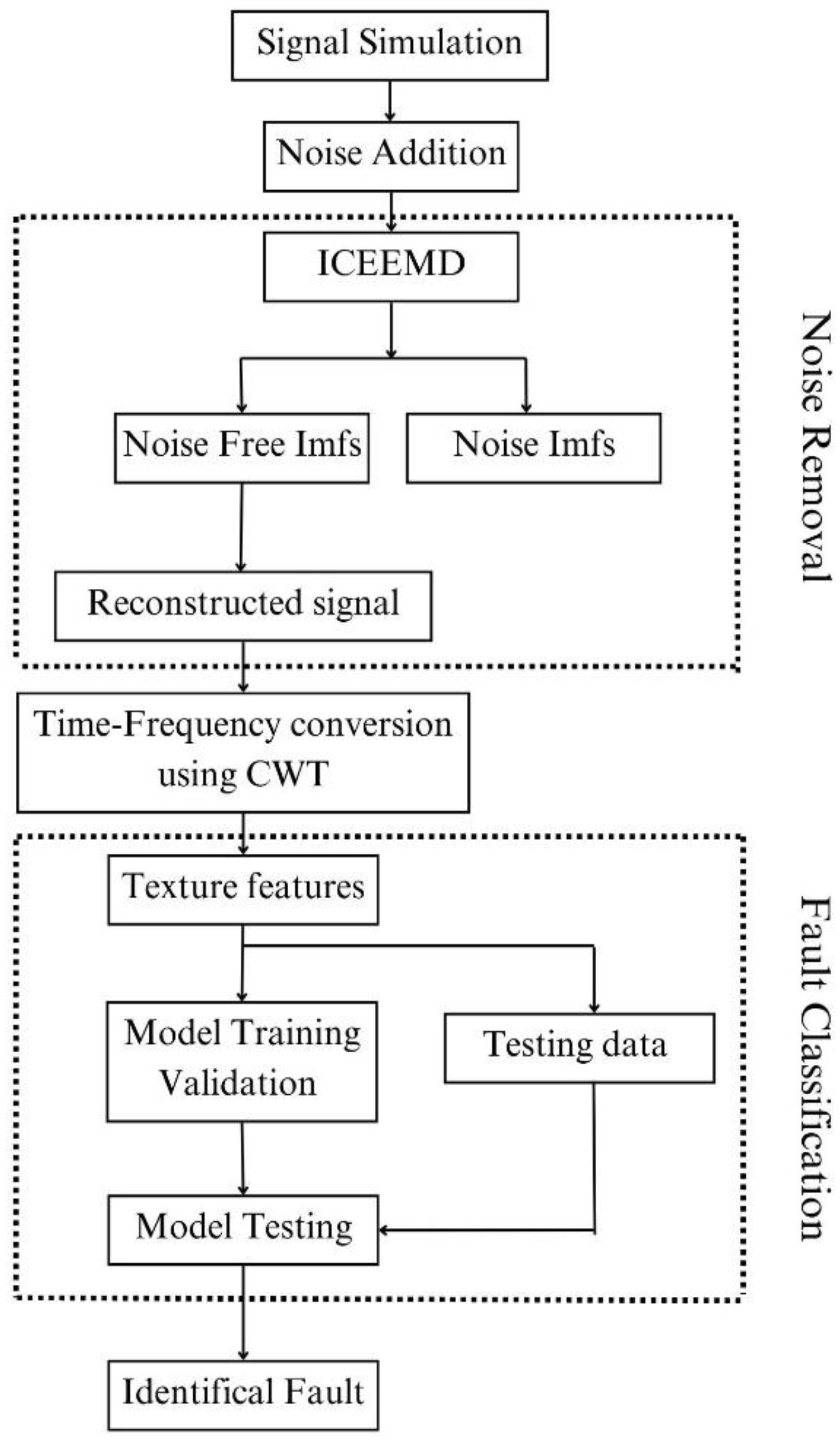
The proposed methodology of the work is shown in Figure 2. The overall process is carried out in five stages: signal simulation, noise removal, TF conversation using CWT, texture feature extraction, and fault classification. The various stages are detailed below.

3.1. Signal Simulation and Noise Addition

The mathematical model discussed in Section 2 is used for signal simulation. In that, the sampling frequency (fs) is set to 10,000 Hz. The amplitude of the fundamental frequency is set to 1.0, the fault frequency amplitude is set to 0.5, and the amplitude of harmonics is set to 0.1. Regarding bearing parameters, the shaft rotates at a frequency of 25 Hz. The bearing consists of 8 balls, each with a diameter of 0.02 m. The pitch diameter is set to 0.1 m. Additionally, the contact angle between the balls and the races is 15 degrees.

Noise is added to the training and testing datasets to ensure comprehensive model validation. Five different SNR values are used, and the results for each noise level are evaluated separately. For each noise level, 100 samples are considered for each fault type, with each sample containing 5000 data points. Consequently, a total of 500 samples are analyzed for each noise level.

3.2. Noise Removal

ICEEMD decomposes the signal into a runs of IMFs in the noise removal step. In ICEEMD, an ensemble of K white Gaussian noise realizations is generated. Next, the first IMF is generated using the below equation.

$${IMF}_1={\displaystyle \frac{1}{K}}{\sum }_{k=1}^{K}EMD(x\left(t\right)+{\in }_1{w}_k(t))$$

where ${\in }_1$ is a scaling factor of noise and $w_k\left(t\right)$ is the white noise. Then, the residue is calculated.

$$r_1=x\left(t\right)-{IMF}_1$$

For each subsequent IMF, noise is added to the residual, continuing until the residual is monotonic or lacks oscillations. ICEEMD has high computational complexity due to multiple noise-assisted decompositions and iterative sifting. It requires substantial memory and processing power, particularly for long signals and large ensemble sizes. Parallel computing is essential for efficient real-time implementation.

After decomposition, the IMFs are analyzed to distinguish between noise components and those carrying meaningful information about the bearing’s condition. This work chooses noise-free IMFs based on their similarity to the original signal. IMFs with a correlation greater than 0.3 are considered noise-free, a threshold set based on the previous literature [16,17]. Noise IMFs are discarded, while noise-free IMFs are retained to reconstruct the vibration signal.

3.3. TF Conversion Using CWT

CWT is used for TFA with the Morse wavelet function in this stage. The Morse wavelet provides a balanced trade-off between time and frequency localization, making it well-suited for analyzing non-stationary signals. Prior studies have demonstrated its effectiveness in machinery fault detection, ensuring a high detection performance without excessive computational complexity [13,18]. The CWT images of all faults, with and without denoising, are shown in Figure 3.

To represent noise signals, the CWT of noise with −4 dB SNR is considered. In the CWT images, the effectiveness of the denoising process is visually evident. The red-colored circles highlight the regions where noise has been effectively removed from the TF representation, demonstrating the suppression of unwanted signal components. Meanwhile, the yellow-colored circles indicate the retained fault frequency components, ensuring that critical fault-related information is preserved. The denoising process enhances the clarity of harmonic structures, resulting in sharper and more distinguishable frequency components. This improvement underscores the effectiveness of combining ICEEMD with CWT in extracting meaningful fault features, thereby improving the fault detection accuracy even in significant noise.

3.4. Texture Feature Extraction

Texture feature extraction involves analyzing the TF representation of the vibration signal obtained from CWT to capture key characteristics indicating the presence of faults. This study employs textural attributes extracted from the gray-level co-occurrence matrix (GLCM). The 14 Haralick features considered are energy, contrast, correlation, variance, homogeneity, sum average, sum variance, sum entropy, entropy, difference variance, difference entropy, and the information measures of correlation (IMC1 and IMC2).

3.5. Fault Classification

After noise removal and feature extraction, the model is trained using these features to learn patterns associated with five different fault types, such as inner race, outer race, ball defects, and cage defects. A multi-layer perceptron (MLP) is used for this purpose. It begins with a feature input layer with Z-score normalization to standardize the input data. This is followed by a fully connected layer with 500 neurons, activated using a ReLU (Rectified Linear Unit) layer to introduce non-linearity. To mitigate overfitting, a dropout layer with a 30% dropout rate is incorporated.

Next, the network includes a fully connected layer with 300 neurons, followed by another fully connected layer with 100 neurons. A final fully connected layer with five neurons is used to classify the data into five categories. The output is processed through a softmax layer, which converts the logits into probability scores, followed by a classification layer, which assigns the final class labels.

The training process is configured using the Adam optimizer, which updates the network weights based on adaptive learning rates. The maximum number of epochs is set to 200, allowing sufficient iterations for learning. The validation dataset is evaluated after every 20 iterations to monitor model performance. The initial learning rate is set to 0.01, balancing convergence speed and stability. At each noise level, 500 samples are used. Among these, 80% (400 samples) are allocated for training the algorithm, 10% (50 samples) for validation, and 10% (50 samples) for testing.

The performance metrics used for comparison include training accuracy, training loss, validation accuracy, validation loss, test accuracy, F1 Score, specificity, precision, and recall (sensitivity).

4. Results and Discussion

The performance of the proposed methodology is verified for various noise levels, and the accuracy is shown in Figure 4.

The results indicate the impact of increasing noise levels (decreasing SNR) on model performance. At SNR = −4 dB, the model achieves 100% accuracy across training, validation, and testing, suggesting that the data are highly distinguishable despite noise. However, as the noise level increases (SNR = −8 dB to −20 dB), a gradual decline in accuracy is observed. The training accuracy drops from 100% to 89.06%, indicating that higher noise levels introduce challenges in feature learning. The validation accuracy fluctuates but remains relatively stable, suggesting that the model generalizes well within the validation dataset. Meanwhile, testing accuracy decreases from 100% to 78%, demonstrating that extreme noise levels affect the real-world fault classification performance. This trend highlights the model’s robustness to moderate noise but also its limitations under severe noise conditions (SNR = −20 dB), where misclassification increases.

The cross-entropy loss for training and validation is shown in Figure 5. It can be observed that the loss gradually increases as the noise level increases.

The detailed analysis of precision, recall, specificity, and F1 Score across different noise levels, as presented in

Table 1. Performance metrics at different SNR levels.

SNR (dB)	Precision	Recall	Specificity	F1 Score
−4	1	1	1	1
−8	0.873	0.897	0.9	0.878
−12	0.918	0.888	0.88	0.892
−16	0.877	0.882	0.88	0.879
−20	0.791	0.795	0.78	0.789

, highlights the model’s performance under varying SNR conditions. The relatively stable recall and specificity indicate that the model can correctly identify most fault conditions.

Further, two comparisons are made to evaluate the effectiveness of the proposed approach. In the first comparison, ICEEMD is replaced with CEEMD; in the second comparison, the MLP classifier is replaced with SVM. The results, shown in

Table 2. Performance comparison of different methods at −20 dB noise level.

Method	Accuracy (%)
	Validation	Testing
CEEMD	84	74
SVM	79	75
Proposed	88	78

, emphasize the effectiveness of ICEEMD for signal decomposition and MLP for classification in enhancing fault detection performance.

The proposed approach is designed to be adaptable to different bearing types and fault modes due to its robust feature extraction and classification framework. By leveraging ICEEMD for signal decomposition and CWT for TF analysis, the method effectively captures fault characteristics across various conditions.

5. Conclusions

The diagnosis of bearing faults is critical for ensuring the reliability and safety of industrial machinery. However, real-world conditions often introduce significant noise, complicating fault detection and reducing the accuracy of conventional diagnostic methods. This study demonstrates that ICEEMD and CWT provide a robust solution for bearing fault identification in noisy environments. By leveraging the noise reduction capabilities of ICEEMD and the TF representation of CWT, the proposed approach effectively isolates fault-related features from background noise. The simulated signal analysis validates this integrated method’s efficacy, showing an improved fault detection accuracy.

Future work can explore the application of this methodology to real-time monitoring systems and extend its use to diagnose other mechanical components, thereby enhancing the predictive maintenance capabilities in various industrial applications.