A Hybrid Machine Learning Approach to Power Load Optimization and Emission Reduction in Rural Microgrids ^†

Abstract

Fluctuating weather patterns challenge renewable energy stability in microgrids, making accurate load forecasting essential. This study focuses on power load forecasting in rural microgrids in the Diamond Harbour sector of Kolkata, India. The current research proposes long short-term memory for weather prediction and artificial neural networks for load forecasting under different climatic conditions. The result shows higher prediction accuracy (R²: 0.8852, MSE: 0.0043), outperforming GRU, SVM, ARIMA, and SARIMA, contributing to Sustainable Development Goals 7 and 13, which is essential for a sustainable and resilient power supply.

1. Introduction and Literature Review

Rural areas often struggle with unreliable electricity. This problem calls for using renewable energy sources (RESs). In regions like Diamond Harbour, India, such innovations can optimize the microgrid performance to meet energy needs, consistently reduce the reliance on fossil-fuel-based energy systems, and, thus, reduce emissions. However, the benefits of microgrids are reduced by the substantial challenges they face in balancing energy supply and demand, mainly because RESs are variable due to their dependence on weather conditions. Therefore, an effective energy management system (EMS) within microgrids ensures these systems operate efficiently and reliably. Achieving this requires using optimal methods that can accurately forecast the energy demand-to-supply ratio, incorporate multiple types of energy, and implement strategies for managing energy storage and distribution while promoting cleaner energy transitions and empowering sustainable rural growth.

Much research has been performed in terms of the energy management of microgrid systems where different techniques are used in the existing methodological framework. A study presented a comparative analysis of three models of photovoltaic systems. Among all these models, the support vector machine (SVM) with the Grey Wolf Optimizer was more effective in fault classification [1]. Also, the inclusion of regions of interest (ROIs) provided a boost to the cloud distribution predictions [2], and the deep learning (DL) adaptive model did quite well in providing high-accuracy results [3], which suggests that the use of these advanced methods is improving the prediction accuracy. Another study surveyed DL models for forecasting solar PV power generation using the ant colony optimization hybrid SVM-GRU model. The results showed high accuracy, which indicates the model’s potential for enhancing actual-time predictions of PV power and enhancing renewables’ application in intelligent grids [4]. Similarly, a study incorporated hybrid models combining ML techniques with real-time weather data for wind power production and, therefore, the stability of microgrids.

Table 1. Performance summary of ML and DL models used in weather forecasting.

Model Type	Variables Considered	Performance Metrics	Ref.
SVM and Gaussian procs Regression	PV power output data	RMSE = 1.1775, R2 = 0.9483, MAPE = 0.1787	[5]
Res-Att-GRU model	Solar irradiance, air T	RMSE = 0.336 kW, MAE = 0.177 kW, MAPE = 12.89%	[6]
PCA combined with ANNs using MDOE	T, H, P, WS, WD, G, SR	MAPE = 6.75%, SD = 6.47 (spring); MAPE = 10.54%, SD = 7.29 (summer)	[7]
ANN forecasting model; 5 MW PV Plant	T, WS, WD, H, Cc	Power saving was nearly 48,000 kWh/year	[8]
RNN-LSTM architecture	SR, WD, T	MSE; MAE, RMMSE, and MedAE; R2 = 0.99	[9]
Encoder–decoder LSTM network	ATu, H, SR	RMSE = 0.9636 mw (sunny), RMSE = 4.0123 mw (cloudy), RMSE = 2.9828 mw (rainy)	[10]

Note: Atmospheric Turbidity (ATu), Cloud Coverage (Cc), Gust (G), Humidity (H), Mean Absolute Error (MAE), Mean Squared Error (MSE), Mean Absolute Percentage Error (MAPE), Pressure (P), Photovoltaic (PV), Root Mean Squared Error (RMSE), Solar Radiation (SR), Standard Deviation (SD), R-Squared (R²), Temperature (T), Wind Direction (WD), and Wind Speed (WS).

provides a concise overview of various ML models involved in weather prediction and includes the specifics of the methods, parameters, and performance metrics. The CAE-PCA model, as well as the SVM-GPR model [5], provides high precision and low error rates. The adaptive learning neural networks and the attentive gated recurrent residual network (ResAttGRU) [6] utilize data on the solar irradiance and temperature to predict the weather with moderate to high accuracy.

Unlike traditional forecasting approaches like ARIMA, SARIMA [11], SVM-GRP [5], and GRU [4], these models have limitations in capturing microgrid systems’ non-linear and dynamic nature, leading to less optimal performance. The novelty of this model lies in its ability to leverage LSTM to capture the temporal dependencies in weather data while using ANN to forecast the load under fluctuating conditions accurately. This dual-model strategy significantly enhances the predictive accuracy, surpassing conventional methods and improving energy management in microgrids. This study presents an innovative solution for optimizing microgrid performance, ensuring a stable energy supply, and reducing emissions in rural areas by addressing these critical challenges. The study’s objectives are as follows:

• Develop and validate hybrid ML models combining LSTM and ANN for energy demand forecasting in rural microgrids while addressing energy efficiency.
• Analyze the model performance under varying weather conditions to ensure its reliability and the adaptability of renewable energy systems in mitigating energy supply fluctuations and associated emissions.
• Enhance the operational efficiency of rural microgrids to reduce the carbon footprints.
• Propose solutions to the energy challenges of the Diamond Harbour region.

To achieve the above-stated objectives, this study will assess (i) LSTM optimization in forecasting and (ii) ANN optimization in energy demand prediction within microgrids, particularly when historical data are limited. It will also assess the variables that determine the execution of these models based on various types of weather.

2. Materials and Methods

2.1. Experimental Setup

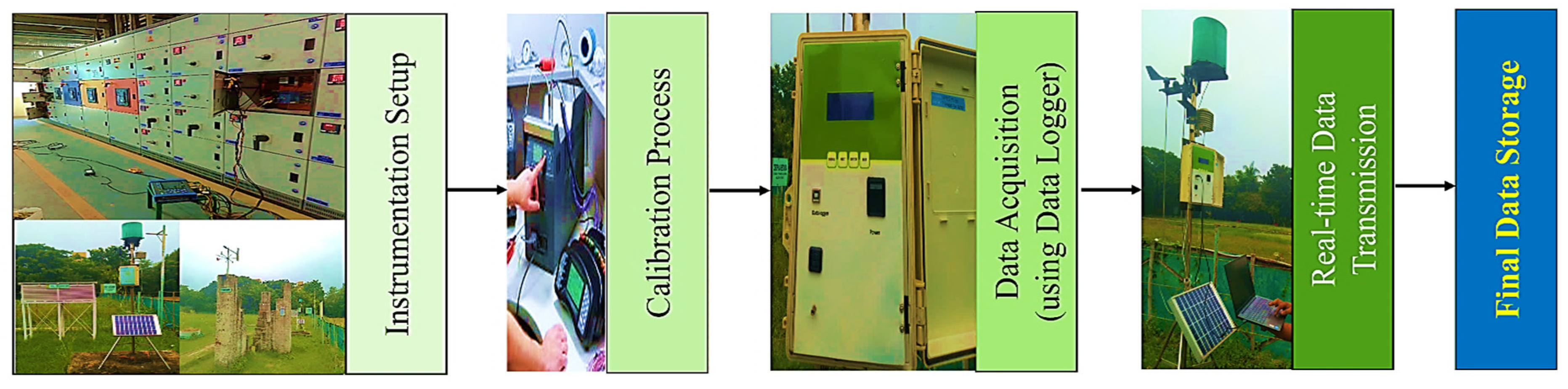
Accurate future meteorological and load data are crucial for designing a sustainable microgrid model applicable to any location globally. Figure 1 shows the experimental flowchart for the data collection. The data acquisition system was based on a single Campbell Scientific CR1000X data logger. Data were obtained using a logger that recorded the required data around the clock. All these data were then forwarded to our data file for use in the data analysis process. The status of the grid was extracted from the university logbook, and the actual energy consumption was obtained through electricity bills provided by the state electricity distribution company (WBSEDCL), which were cross-checked with the smart meter installed at the university.

Table A1. Instrumentation details.

Instrument	Model	Maker	Range	Accuracy	Tolerance	Calibration
Pyranometer	SMP11	Kipp & Zonen	0 to 2000 W/m2	±2%	±5 W/m2	Annually
Anemometer	WAA151	Vaisala	0 to 60 m/s	±0.10 m/s	±0.5 m/s	Bi- annually
Temperature Sensor	HMP155A	Campbell Scientific	−79 to +59 °C	±(0.06 + 0.006 × temp.) °C	±0.2 °C	Quarterly
Smart Meter	E650	Landis + Gyr	0 to 5000 kW	Class 0.2 s (±0.2%)	±0.5%	Annually
Data Logger	CR1000X	Campbell Scientific	N/A	24-bit A/D converter	N/A	N/A

summarizes the instruments’ specifications, accuracy, and operational ranges. Sensors were strategically placed across the site to minimize the environmental interference after the calibration [12].

2.2. Data Collection

The data were collected at the Neotia University (TNU), Diamond Harbour, Kolkata, West Bengal, India; the coordinates for it are 22°15′38.87″ N and 88°11′44.45″ E. The climate of this area differs considerably in different seasons. Data collection was performed from 1 January 2019 to 31 December 2023, and data were recorded at one-hour intervals. All the seasonal changes expected for the region were incorporated.

2.3. Overall Flow

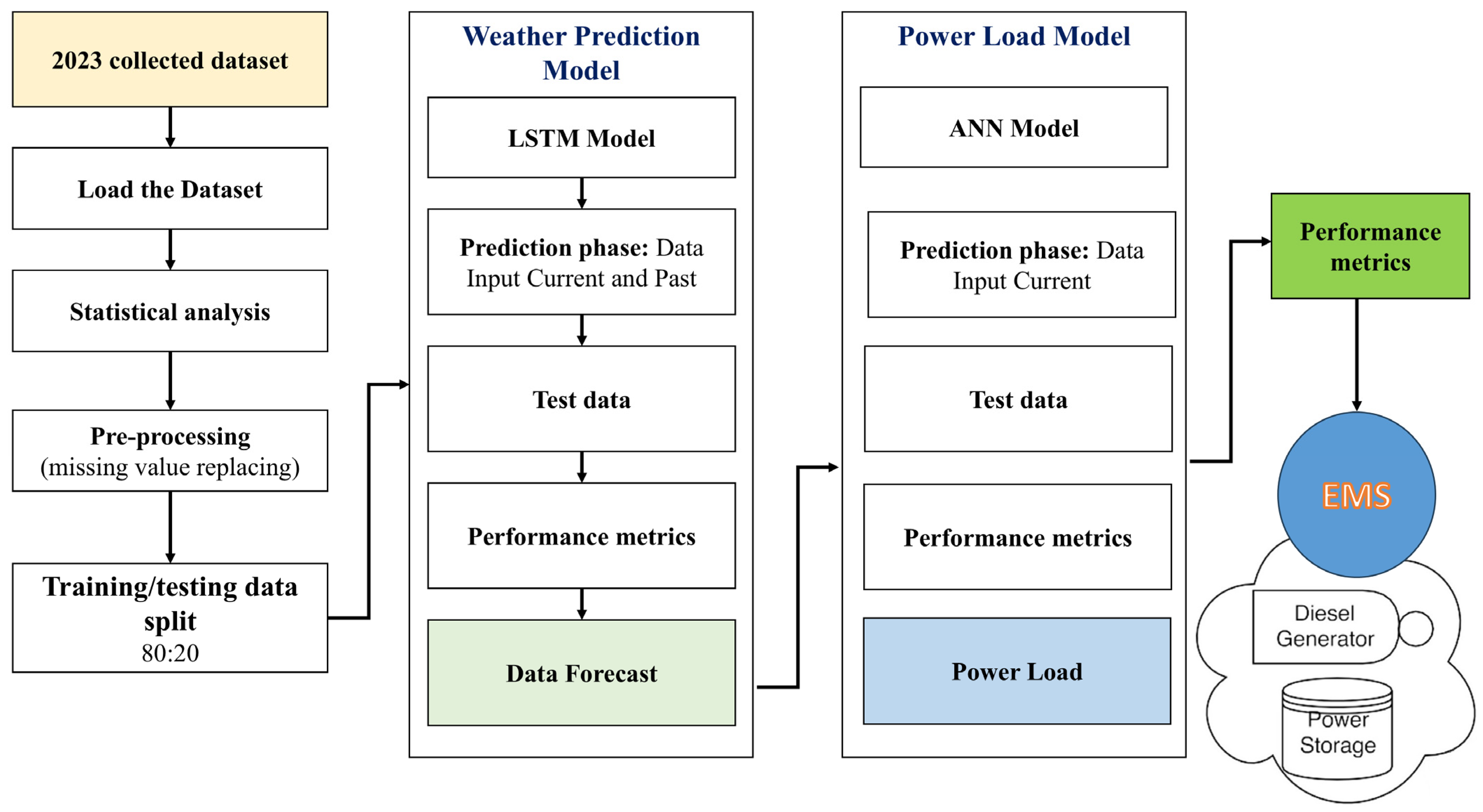
This study involved developing and implementing a hybrid ML model for assessing the behavior of community power loads in rural microgrids. As stated, the approach had several significant steps: data acquisition/pre-processing, model development and training, and model evaluation, as outlined in Figure 2. In the beginning, the experimented dataset was loaded. After this, statistical analysis was carried out to assess the statistical characteristics using the Pearson correlation and pairwise correlation approaches. The data pre-processing involved handling missing values and inconsistencies. Then, the dataset was split into an 80/20 training and testing data ratio. The data were then fed into the proposed LSTM-ANN model, and the performance metrics were analyzed.

2.4. Pre-Processing of Data

After data collection, the data were then pre-processed to ensure uniformity in identifying and rectifying anomalies within the dataset, which involved several critical steps. First, the independent variable scales were standardized to reduce the dominance of other variables in the analysis and maintain the integrity of the model. In case of data gaps, an attempt was made to fill them based on the data’s nature and distribution. This included the mean substitution, interpolation, and other algorithms. Noise reduction procedures were employed to eliminate outliers and enhance the nature and quality of the obtained dataset.

2.5. Model Architecture

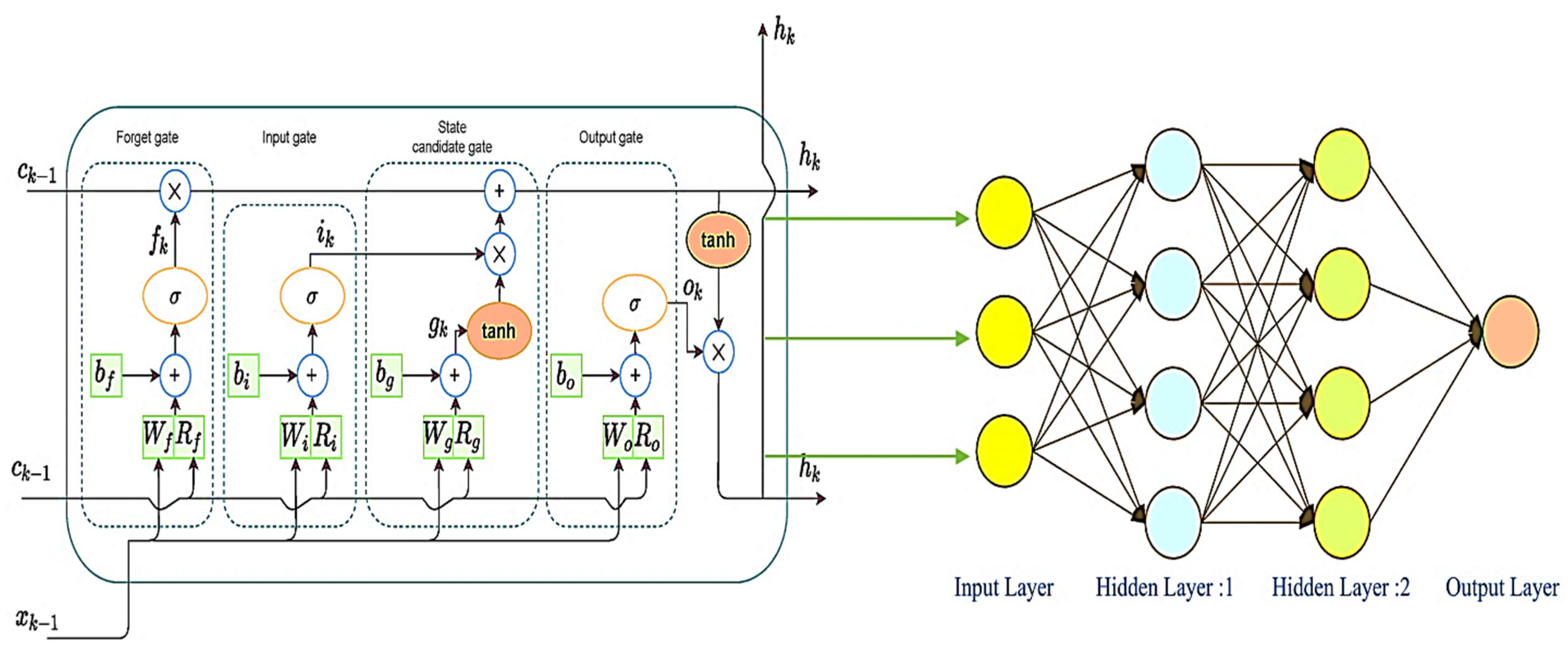
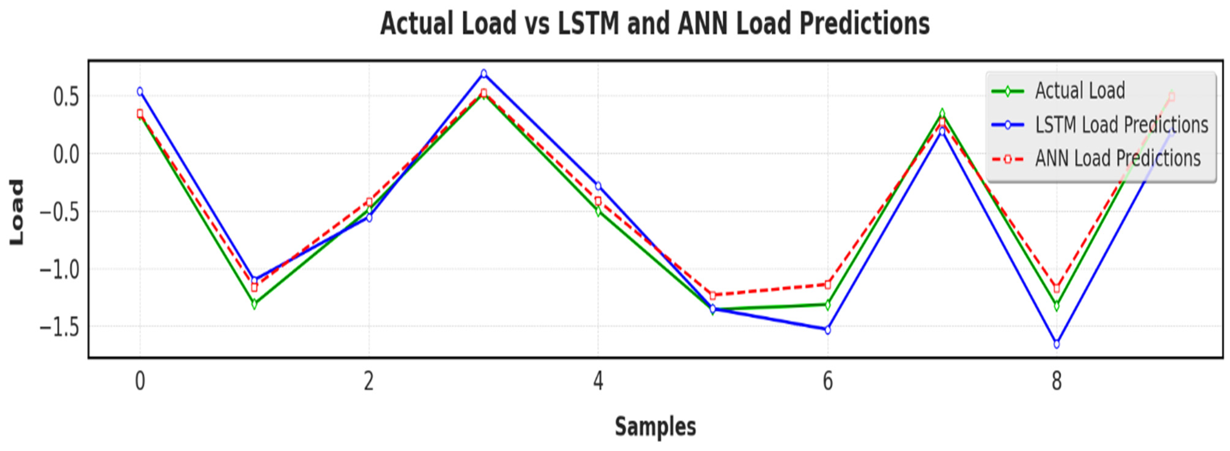
Figure 3 shows the overall architecture of an integrated model (LSTM-ANN) for load forecasting in rural microgrids. The LSTM model generates the forecast data from the experimental data inputs. The predicted LSTM data thus feed the ANN model to accurately predict the current-time power demand forecasts. These values are then fed into the EMS to manage traditional power generation.

LSTM Model for Weather Prediction: The input layer takes in sequences of weather data; the shape of the input is defined by the look_back period and number_of_features. Such a configuration allows the model to predict a history of weather observations. The LSTM layer-1 comprises 50 units, and return_sequences = True to pass values to the next LSTM layer. This layer captures the temporal dependencies usually embedded in the sequential data. The LSTM layer-2 comprises 50 units, and return_sequences = False to return only the last output in the sequence, which summarizes information captured by the first layer into a final feature vector. Following the LSTM layers, a dense layer-1 with 25 nodes is introduced to make the feature space compact, simplifying the model without losing essential features. The output layer consists of the number_of_features neurons, representing the various weather parameters. The Adam optimizer is used in the model for its adaptive learning capabilities and efficiency in processing large datasets. The MSE loss function is used to reduce the errors in the prediction process and improve the accuracy.

ANN Model for Power Demand Prediction: The input features for the ANN model are the weather predictions generated by the LSTM model, allowing the ANN to power the temporal patterns identified by the LSTM. The dense layer-1 consists of 64 neurons. The rectified linear unit (ReLU) is used to initiate non-linearity in the model. This enables the ANN to map the non-linear relations of the weather aspects regarding the power demand. A dense layer-2 with 32 neurons allows for the further processing of the feature space with the activation function of the ReLU being used to enhance the training facility and network accuracy. The output layer contains a single unit with a linear activation task, which provides a continuous function that produces the predicted power load. Like the LSTM model, the Adam optimizer also compiles the ANN. The MSE is used as the loss function to measure and rectify prediction errors during training.

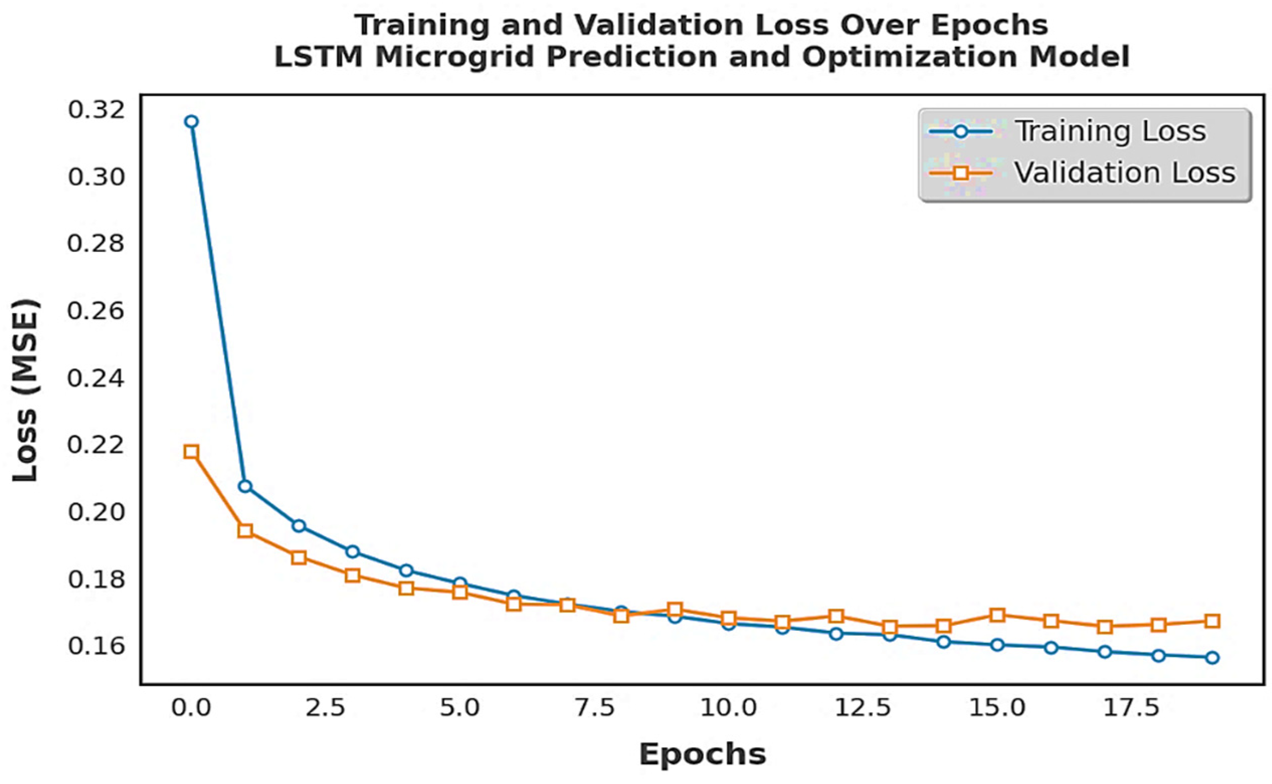
2.6. Training Configuration

The LSTM model was trained on experimental data to predict future data. Key hyperparameters, such as the number of LSTM layers, units per layer, batch size, and epochs, were optimized. The feature selection was systematic in the grid search to balance accuracy and efficiency by determining the best combinations of hyperparameters and the best configuration for the LSTM model. The LSTM model used in this study was trained with a batch size of 500 instances. The training parameters were fine-tuned through experiential approaches to improve the model execution. The chosen parameters involved a learning rate of 2.5 × 10⁻⁴, a past history window length of 30-time steps, and 5 output cells. The architecture comprised 300 LSTM units distributed across 4 hidden layers. The training process was set to terminate when the error loss reached 1.0 × 10⁻⁵ or after completing a maximum of 300 epochs, whichever came first. For forecasting, the LSTM model provided 5 outputs, each predicting the weather conditions 10 min ahead, resulting in a total prediction horizon of 50 min.

The ANN model was then trained using the weather prediction from the LSTM as an input variable to predict the power load. This included multiple layers that used the rectified linear unit ReLU initiation task, which is known to speed up convergence during training to achieve high accuracy while simultaneously reducing the computational costs. The ANN model for the power demand prediction contained an input layer, one or more hidden layers, and an output layer. Following empirical adjustments, the ANN optimal configuration for the power forecasting included 4 hidden layers with neuron counts of 300, 500, 500, and 300, respectively. The batch size was adjusted to 500 instances, and the model trained over 200 epochs. ReLU activation functions were applied to each neuron in the hidden layers, chosen for their effectiveness in mitigating vanishing gradient issues and enhancing the learning efficiency in deep networks.

To train the model, the dataset was split into training (80%) and testing (20%) subsets. The training subset was used to build the model, while the testing subset was used for the model performance evaluation. Feature scaling was applied to the dataset to prevent bias in the training process. Equations (1) to (15) explain the model implementation algorithm.

2.6.1. LSTM Layer Implementation

The input sequence for the LSTM layer is:

$$X^{\left(LSTM\right)}; X_t=\left[x_t,x_{t-1},\dots ,x_{t }\right]$$

(1)

The hidden state at a time $t$ is denoted as:

$$h_t=\mathrm{L}\mathrm{S}\mathrm{T}\mathrm{M}\left(X_t^{\left(LSTM\right)},h_{t-1}\right)$$

(2)

Here, $h_t$—hidden state at time t, and $h_{t-1}$—hidden state at a previous time step.

The key processes for the LSTM cells at each time step are as follows:

• Forget gate: determines which parts of the earlier cell state should be carried forward to the next step:

$$f_t=\sigma \left(W_f\cdot \left[h_{t-1},x_t\right]+b_f\right)$$

(3)

• Input gate: chooses which current input values should be updated in the cell state:

$$i_t=\sigma \left(W_i\cdot \left[h_{t-1},x_t\right]+b_i\right)$$

(4)

• The cell state (${\tilde{C}}_t$) is produced using the hyperbolic tangent function:

$${\tilde{C}}_t=\mathrm{t}\mathrm{a}\mathrm{n}\mathrm{h}\left(W_C\cdot \left[h_{t-1},x_t\right]+b_C\right)$$

(5)

The new cell state ${\tilde{C}}_t$ is then updated as:

$$C_t=f_t\cdot C_{t-1}+i_t\cdot {\tilde{C}}_t$$

(6)

• Output gate: controls the following hidden state, which will be utilized for the predictions. It is computed as:

$$o_t=\sigma \left(W_o\cdot \left[h_{t-1},x_t\right]+b_o\right)$$

(7)

where the weight matrices: $W_f$, $W_i$, $W_C$, $W_o$; bias vectors: $b_f$, $b_i$, $b_C$, $b_o$; and hyperbolic tangent function: $\mathrm{t}\mathrm{a}\mathrm{n}\mathrm{h}$

The LSTM model output is:

$$y_t=\sigma \left(W\cdot h_t+b\right)$$

(8)

The LSTM model loss function is given by the

$$\mathrm{MSE}: {\mathcal{L}}_{LSTM}={\displaystyle \frac{1}{N}}{\sum }_{i=1}^N{\left(y_i-{\widehat{y}}_i\right)}^2$$

(9)

where the true value is ($y_i$) and the predicted value is (${\widehat{y}}_i$).

2.6.2. ANN Layer Implementation

The ANN model input is denoted as:

$$a_1=X^{\left(ANN\right)}$$

(10)

Each layer in the ANN performs the following operations:

First layer: the first layer computes the pre-activation $z_2$ and activation $a_2$:

$$z_2=W_1\cdot a_1+b_1$$

(11)

$$a_2=\mathrm{R}\mathrm{e}\mathrm{L}\mathrm{U}\left(z_2\right)$$

(12)

Second layer: the second layer computes the pre-activation $z_3$ and activation $a_3$ as:

$$z_3=W_2\cdot a_2+b_2$$

(13)

$$a_3=\sigma \left(z_3\right)$$

(14)

where $\sigma \left(z\right)$ sigma—sigmoid activation function, often used in the output layer for binary classification tasks, produces a value 0~1 (interpreted as a probability).

Loss function and training ANN:

$$\mathrm{MSE} - {\mathcal{L}}_{ANN}={\displaystyle \frac{1}{N}}{\sum }_{i=1}^N{\left(y_i-{\widehat{y}}_i\right)}^2$$

(15)

where the activations in the ANN layers: $a_1$, $a_2$, $a_3$;

Pre-activations in the ANN layers: $z_2$, $z_3$

The backpropagation algorithm updates the weights and biases by estimating the gradients of the loss function with regard to each parameter. Later, the gradients are utilized to adjust the parameters to minimize the loss.

2.7. Performance Evaluation Metrices

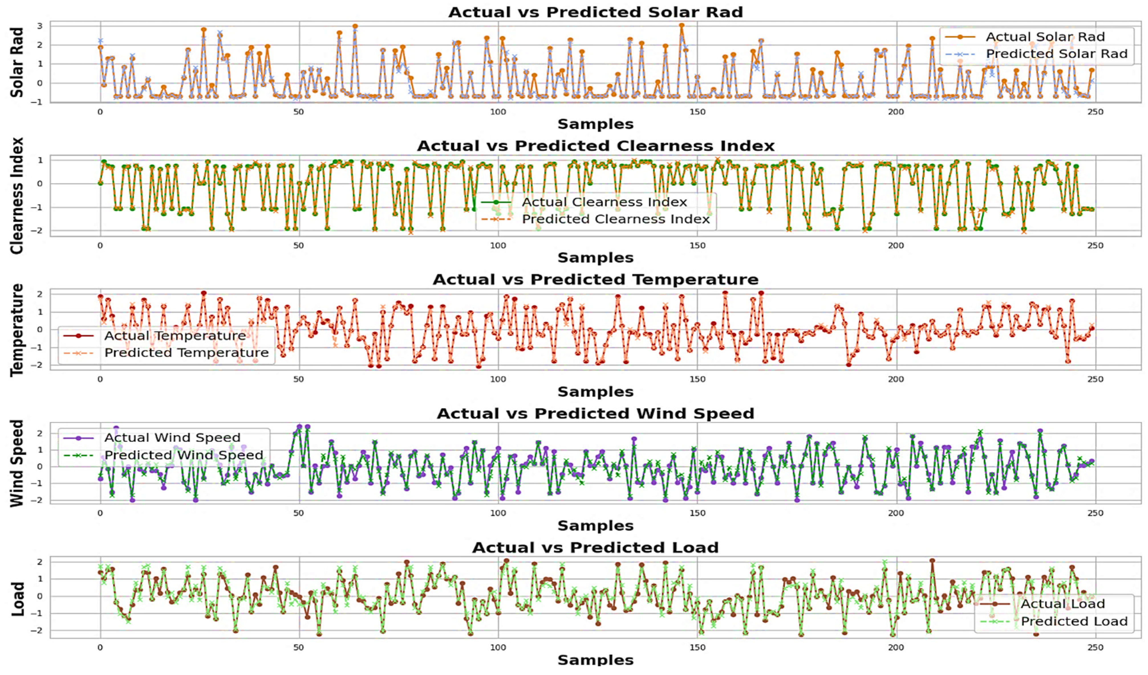
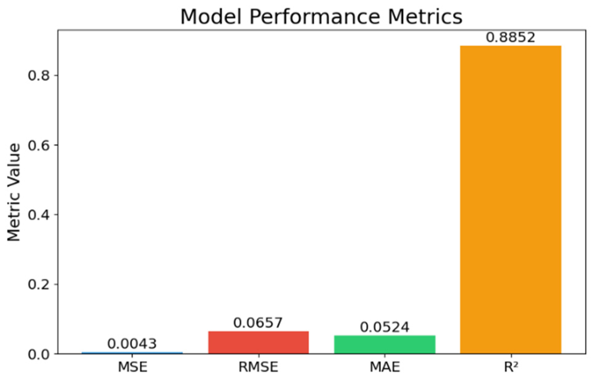
The performance of the proposed LSTM-ANN model was evaluated using statistical metrics: MAE, RMSE, MSE, and R². The MAE measures the average error magnitude, the RMSE emphasizes large errors, the MSE minimizes the deviations, and the R² indicates the model accuracy. These metrics help compare LSTM-ANN with the ARIMA, SARIMA, and GRU models. Lower MAE, RMSE, and MSE values signify better accuracy, while a higher R² suggests strong predictive performance.

3. Results and Discussion

3.1. Forecast Analysis: LSTM

Figure 4 and Figure 5 show comparative analyses of the actual and LSTM-predicted values over time. The visual illustration shows the accuracy of the forecasting model.

As presented in Figure 4, there is a very close relationship between the predicted load and the actual load; thus, it can be well understood that the model is running efficiently. Figure 5 shows the closeness of the predicted line to the actual data line, which signifies the model’s accuracy and reliability in terms of other forecasting values.

The training and validation loss can be identified in Figure 6. The model’s training loss (blue curve) starts at a high value of 0.33 (approx.) at epoch 0, exhibits a sharp drop, and flattens out around an MSE of 0.152 after five epochs. The validation loss (red curve) also increases gradually, and the initial MSE of 0.22 and decreasing to 0.155 (approx.) by the fifth epoch. After this point, both losses keep declining slightly; the final training and the validation losses are at about 0.149 and 0.158 by the 20th epoch.

It is viewed that the LSTM model has a high generalization ability with less overfitting. This is specifically important in terms of using the model for microgrid prediction and optimization, where the prediction and optimization capabilities of the model determine the overall quality of the real microgrid load and energy management process. These results underscore the robustness of the LSTM architecture in handling the complex, temporal data characteristic of microgrid operations.

3.2. Load Optimization: ANN

This section assesses the load optimization accuracy of the proposed ANN model. As seen in Figure 7, the power load values were well predicted; this proves the efficiency of the developed model.

A comparative assessment of the models is shown in Figure 8, where the LSTM predictions are, in general, good at catching macro behavior, while during specific periods of load demand, they tend to differ significantly; for instance, underestimating at sample points 2 and 7 by 0. 2 units. This indicates challenges in terms of the LSTM’s ability to adapt to rapid load changes, which are common in microgrid systems with fluctuating weather conditions. In contrast, the ANN model can be seen outperforming, and in general, it tracks the actual load values better, especially in the fluctuating period. For instance, at key points such as samples 3 and 8, the ANN predictions nearly overlap with the actual values, with a maximum deviation of only 0.05 units. This suggests that the ANN has this associative learning nature, which is best suited when used in the short-term load forecasting of unpredictable weather conditions.

3.3. Proposed Model Performance Analysis

The bar chart in Figure 9 illustrates the proposed model performance analysis. The MAE, RMSE, and R² values were used to evaluate the accuracy and effectiveness of the proposed model. The RMSE of 0.0657, MAE of 0.0524, and R² value of 0.8852 indicate a highly accurate predictive capability.

These metrics demonstrate the model’s robustness in handling complex temporal data, validating its effectiveness for microgrid prediction and load optimization.

State-of-the-Art Analysis

A state-of-the-art analysis of different models for forecasting data was conducted. The performance metrics used in the assessment included the MAE and R², with the results visualized in

Table 2. Evaluation metrics for the traditional and proposed models.

Model	R2	MAE
GRU [4]	0.8013	0.2120
SVM [5]	0.8469	0.1512
LSTM-ANN (Proposed Model)	0.8852	0.0524

. The GRU and SVM models showed a reasonably good level of predictiveness, with a recorded R² of 0.8013, 0.8469, and an MAE of 0.2120, 0.1512. The LSTM model performed best with the highest R² of 0.8852 and an MAE of 0.0524. On the other hand, poor predictability was observed when using the ARIMA, SARIMA [11], and Prophet models. The MAE values were notably high (ARIMA: 0.8806, SARIMA: 0.8814, Prophet: 0.8817), reflecting substantial prediction errors. This inadequacy is primarily recognized due to their limitations in handling the data’s complexity and non-linear patterns.

Overall, these performances indicate that the hybrid LSTM-ANN approach can be a valuable tool for improving energy management in microgrids, providing a good response for short-term and long-term load forecasting even under adverse situations.

4. Conclusions

The hybrid LSTM-ANN model demonstrated superior accuracy in predicting the power load compared with the traditional approaches. The model effectively addressed complex non-linear relationships and temporal dependencies, which are key characteristics of vital microgrid operations. By addressing the variability of the RES under different weather conditions, the model enhanced the operational efficiency, ensured energy reliability and load optimization, and significantly reduced the carbon footprints. This study provides a robust framework for sustainable energy management in rural microgrids. Future studies should incorporate socio-economic indicators, such as population growth and energy consumption behavior. Such additions could enhance the performance of the given model and provide timely and reliable energy management solutions. This study advances data-driven approaches to climate-resilient rural electrification, supporting global decarbonization goals.