Automatic Detection of Defects Using Active Thermography ^† †

Abstract

The increase in composite material waste from the aviation and wind energy sectors will become a significant environmental challenge in the near future. This escalation is attributed to the enhanced use of new, advanced composite materials, such as Glass Fiber Reinforced Polymer (GFRP). Despite their benefits, the disposal of these materials at their end-of-life poses considerable environmental and logistical challenges. Assessing the condition of these materials is thus pivotal to develop sustainable strategies for their recycling, reusing, or repurposing. This study investigates the use of Non-Destructive Testing (NDT) techniques, with a focus on Active Thermography, to evaluate GFRP components’ suitability for sustainable management without compromising the material integrity. This research highlights the use of Active Thermography for extensive, non-invasive inspections, due to its capability to inspect a large area quickly using external energy heating. It delves into Pulse Phase Thermography (PPT) and Principal Component Thermography (PCT), two advanced signal post-processing techniques, tested on GFRP materials with purposefully induced defects. Finally, an automated method based on the Signal-to-Noise Ratio (SNR) value is implemented for defect detection, with which defects of a 5 mm diameter and a 3 mm depth can be detected. The document elaborates on the theoretical principle of NDT, PPT, and PCT, details the experimental methodology and specimens, and analyzes the outcomes of employing these techniques, drawing comparisons between them.

1. Introduction

Glass Fiber Reinforced Polymer (GFRP) is a composite material that consists of a polymer matrix and glass fibers. Due to its properties such as high strength, flexibility, or stiffness, it is a material used in different applications, including electronics, automobiles, and aviation and aerospace. However, due to fatigue and impact damage, different kinds of defects that can reduce the strength and stiffness of GFRP components, such as delamination, fiber crack, and porosity, may be induced in the GFRP laminates during its use [1].

To ensure the good condition of GFRP, Non-Destructive Testing (NDT) is usually used. NDT is a group of testing techniques used to evaluate materials and detect defects without causing damages [2]. One of the most popular NDT methods is InfraRed Thermography (IRT), based on infrared radiation. This technique is dedicated to the acquisition and processing of thermal information [3]. Inside the group of IRT, Pulsed Thermography is one of the most common active thermography testing methods; i.e., an external heat source is used to stimulate the materials under tests is required, as shown in Figure 1.

However, Pulsed Thermography is not perfect and has some problems such as non-uniform surface heating, lateral heat diffusion, or environmental noise. To solve these problems as much as possible, various signal post-processing techniques exist. In this paper, we particularly focus on Pulsed Phase Thermography (PPT), which is based on Discrete Fourier Transform (DFT), and Principal Components Thermography (PCT), which is based on Principal Components Analysis (PCA). To test the effectiveness of both the PPT and the PCT methods, the Signal-to-Noise Ratio (SNR) is subsequently used.

2. Active Thermography

Active Thermography is dedicated to the acquisition and processing of thermal information. Its main advantages are that it is in real time, which enables high speed scanning, and it provides two-dimensional thermal images, which allow a comparison between areas of the target [4].

Pulsed Thermography involves the use of a heat source, usually with halogen lamps, microwaves, or laser induction as a heating source [5], to stimulate an object with a heat pulse. An infrared camera records a video of the object to measure the heating and cooling process on the object’s surface, described by the following equation:

$$T(z,t)=T_0+{\displaystyle \frac{Q}{e\sqrt{\pi t}}}exp\left(-{\displaystyle \frac{z^2}{4\alpha t}}\right),$$

(1)

where T is the temperature function, $T_0$ is the initial temperature, Q is the energy on the surface, $e=\sqrt{k\rho c_p}$ is the material’s thermal effusivity, $\alpha ={\displaystyle \frac{k}{\rho c_p}}$ is the material’s thermal diffusivity, k is the thermal conductivity, $\rho$ is the density, and $c_p$ is the specific heat capacity [6].

At the surface ($z=0\mathrm{mm}$), Equation (1) can be rewritten as

$$T(t)=T_0+{\displaystyle \frac{Q}{e\sqrt{\pi t}}}.$$

(2)

If the composite has homogeneous materials, its thermal diffusivity and conductivity are similar. However, the material of the defective area has different parameters, resulting in a distinct thermal behavior. This difference forms the theoretical basis for Pulsed Thermography.

2.1. Pulsed Phase Thermography

Initially developed by Margado and Marinetti [7,8], Pulsed Phased Thermography is a thermal image sequence post-processing method that involves the calculation of the phase of a thermal image sequence using a Discrete Fourier Transform, which is computed with the following formula:

$${\mathcal{F}}_n=\Delta t\sum _{k=0}^{N-1}T(k\Delta t)expi2\pi kn,$$

(3)

where N is the number of thermal images, $i^2=-1$ is the imaginary number, and $\Delta t$ is the sampling time interval. As a complex number, Equation (3) can be rewritten as the sum of the real (${\mathrm{Re}}_n$) and imaginary (${\mathrm{Im}}_n$) parts of the transform sequence:

$${\mathcal{F}}_n={\mathrm{Re}}_n+{\mathrm{Im}}_n.$$

(4)

To analyze the amplitude and the phase of every harmonic frequency Fast Fourier Transform is used as a quick algorithm of DFT. Amplitude (${\mathrm{A}}_n$) and phase angle (${\varphi }_n$) are expressed as

$${\mathrm{A}}_n=\sqrt{{\mathrm{Re}}_n^2+{\mathrm{Im}}_n^2},$$

(5)

$${\varphi }_n={tan}^{-1}\left({\displaystyle \frac{{\mathrm{Im}}_n}{{\mathrm{Re}}_n}}\right).$$

(6)

With phase images of DFT results, defect regions are emphasized.

2.2. Principal Components Thermography

Principal Components Analysis is a statistical technique used to identify specific patterns in large datasets containing a high number of features per observation and analyze them so as to enable the depicting of similarities and differences of specific patterns. PCA reduces the dimensionality of a dataset. This is accomplished by linearly transforming the data into a new coordinate system where the variation in the data can be described with fewer dimensions than the initial data [9,10]. The use of PCA in post-processing thermographic data is called Principal Components Thermography and was proposed by Rajic [11].

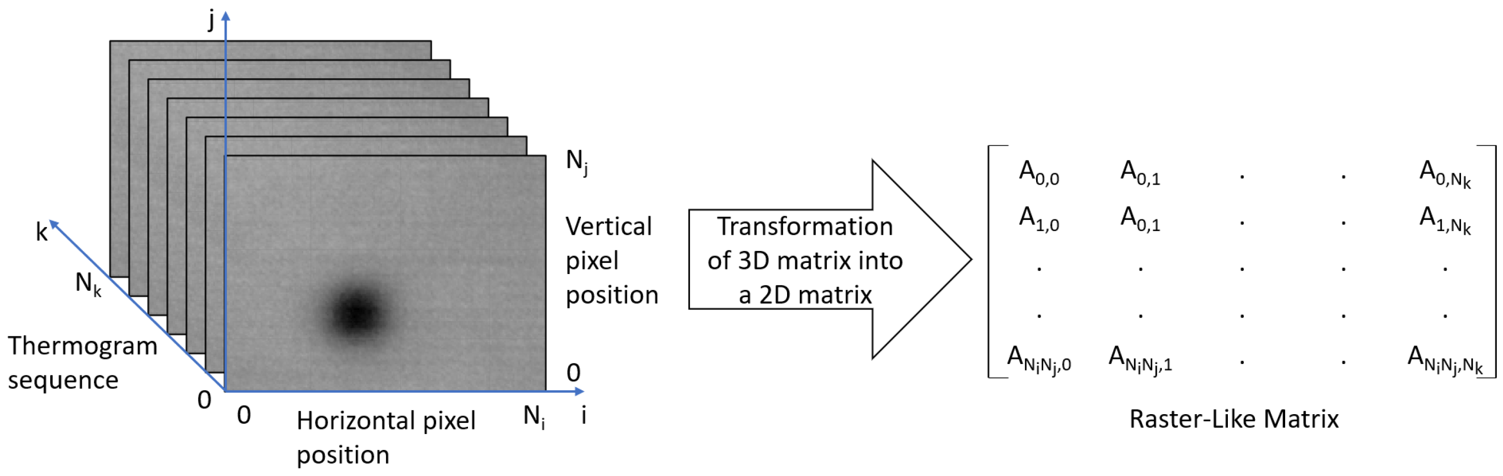
Consider the thermogram sequence as a 3D matrix composed of $N_k+1$ thermograms whose dimensions are $(N_i+1)\times (N_j+1)$. In order to apply PCT to the thermogram sequence, this 3D matrix is transformed into a 2D matrix of dimension $((N_i+1)(N_j+1))\times N_k+1$ by the following equivalence:

$$B[i,j,k]=A[j+i·(N_j+1),k],i\in [0,\dots ,N_i],j\in [0,\dots ,N_j],k\in [0,\dots ,N_k],$$

(7)

where $B[i,j,k]$ is the element of the 3D matrix in row i, column j, and thermogram number k, and $A[i,k]$ is the element of the 2D matrix in row i and column k. This 2D matrix is called a raster-like matrix. Each column of the raster-like matrix represents one thermogram of the sequence, and each row represents temperature evolution of one pixel, as shown in Figure 2.

The raster-like matrix is decomposed with the Singular Value Decomposition, a factorization of a matrix into three matrices, by the following structure:

$$A=US{V}^T,$$

(8)

where U is an $(N_i{N}_j)\times (N_i{N}_j)$ orthogonal matrix, V is an $N_k\times N_k$ orthogonal matrix, and S is an $(N_i{N}_j)\times N_t$ diagonal matrix with its elements uniquely determined by the singular values of A sorted from highest to lowest.

In the described factorization, the columns of the matrix U represent a set of orthogonal statistical models known as the Empirical Orthogonal Functions, $EOFs$. If $EOF$ images are depicted, each $EOF$ corresponds to the respective most characteristic data variability, i.e., $EO{F}_1$ is the first most characteristic data variability, $EO{F}_2$ is the second, etc. In $EO{F}_2$, a distribution is obtained that characterizes a non-uniform field where spatial distribution can be correlated with a contrast signal, which occurs due to the defect in the sample. Therefore, $EO{F}_2$ of PCT gives an image that characterizes the defects embedded in the observed sample [12].

3. Signal-to-Noise Ratio

Before the post-processing techniques, the Signal-to-Noise Ratio [13] measure is applied for the automatic detection of defects.

SNR is a measure that compares the level of a desired signal to the level of background noise. SNR is used to refer to the ratio of useful information to irrelevant data and is defined by the following equation:

$$\mathrm{SNR}=20{log}_{10}\left({\displaystyle \frac{|S-N|}{{\sigma }_N}}\right)dB,$$

(9)

where S is the average value of the signal area, N is the average value of the noise area, and ${\sigma }_N$ is the standard deviation of the noise area.

In respect to the quantitative evaluation, a defect is detected if $\mathrm{SNR}>1$ dB, but it must be noted that defects are more clearly identified if the SNR value is greater.

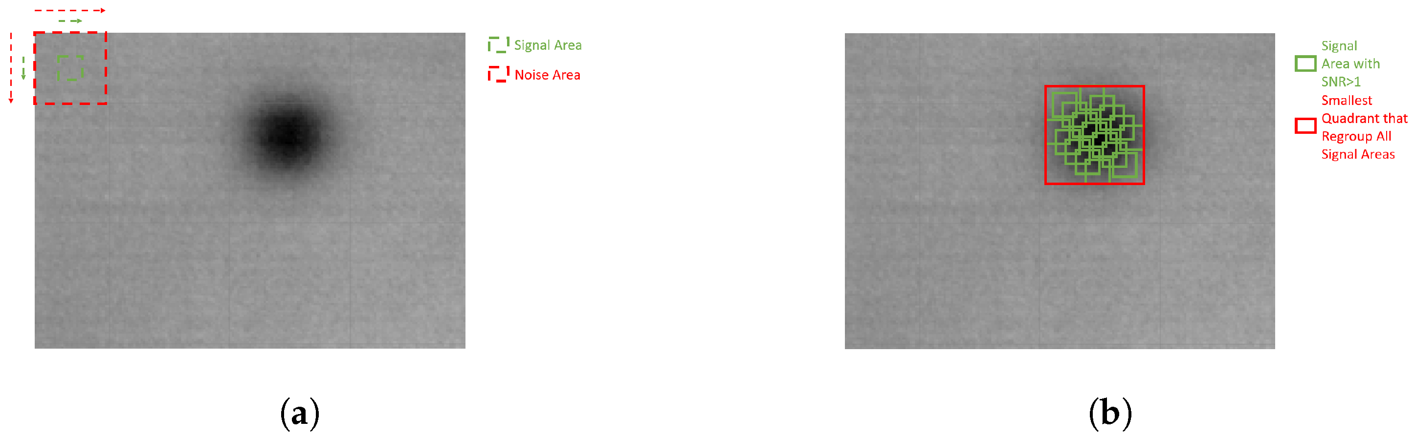
For the automatic detection, we select a $9\times 9$ quadrant as the signal area, and a $27\times 27$ quadrant with the signal area in the center as the noise area. We move pixel by pixel the two areas until the entire image is filled, as in Figure 3a. When more than 4 signal areas with $\mathrm{SNR}>0$ intersect with each other, we regroup them in a larger quadrant and take this as a defect, with the higher SNR of the little quadrants taken as the SNR, as in Figure 3b.

4. Data Information

4.1. Calibration Plate

For the purpose of comparing the different post-processing techniques, they have been applied to a real GFRP piece with artificial defects. In Figure 4a, the test piece is shown. In Figure 4b, the map of the defects can be seen.

The specimen is made of 12 plies of glass-fiber filled with epoxy. Each ply has a depth of 0.83 mm and is numbered from 1 to 12, where Ply 12 is the closest to the surface in which the temperature is measured. The total thickness of the piece is 10 mm. In the specimen, 25 numbered half way hole defects exist; 10 of them are circular in shape, and the rest of them are square-shaped. All defects are found at three different depths: 2.5 mm, 5 mm, and 7.5 mm. In Figure 4a, it can be seen that some defects are observable to the naked eye due to the proximity of the half way holes to the surface.

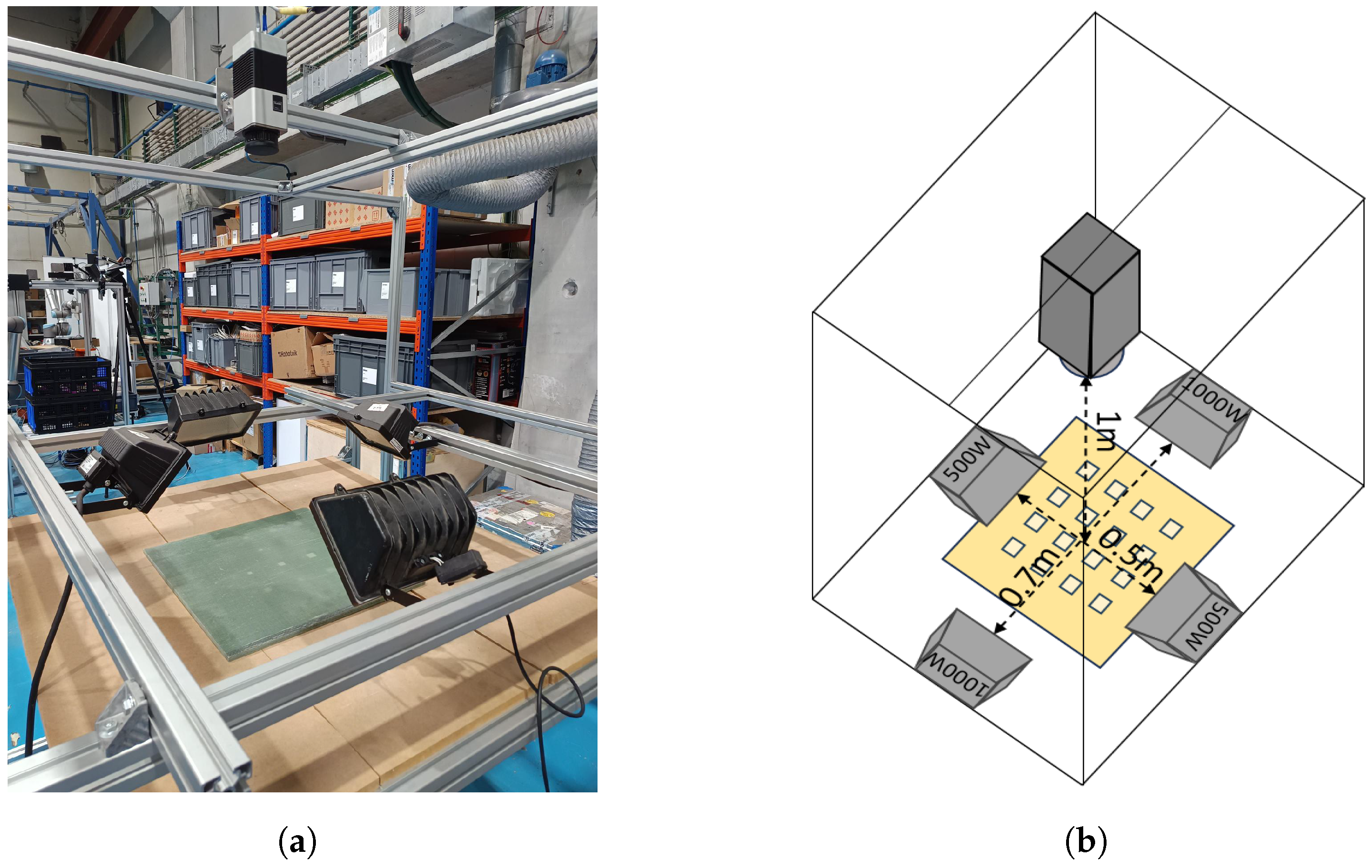
4.2. Setup

In the experiment, four halogen lamps, two of them of 1000 watts at a distance from each other of 70 cm and the other two of 500 watts at a distance from each other of 50 cm, were used as the heat source. The lamps were turned on for 60 s to heat the specimen. Then, the lamps were turned off and the temperature decay was recorded for another 60 s.

The experiment was recorded using an InfraTec VarioCAM^® HD Head 800 [14]. The spectral range of this camera is between 7.5 and 14 µm and has a temperature measure range between −40 and 2000 °C. The resolution of the camera is of (1024 × 768) pixels. Though the camera is able to record with a frame rate of 240 Hz, the experiment was recorded at 30 Hz to reduce the number of acquired images. The distance between the camera and the piece of GFRP was 100 cm.

In Figure 5a, the setup is shown. In Figure 5b, a scheme of the setup can be seen.

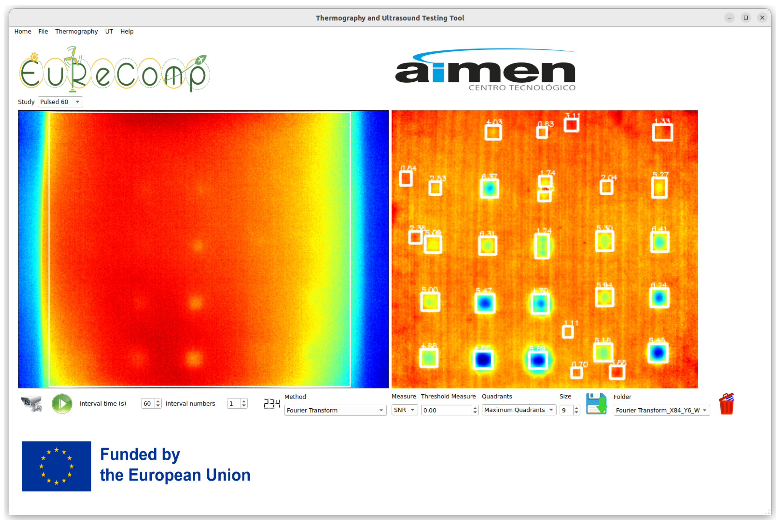
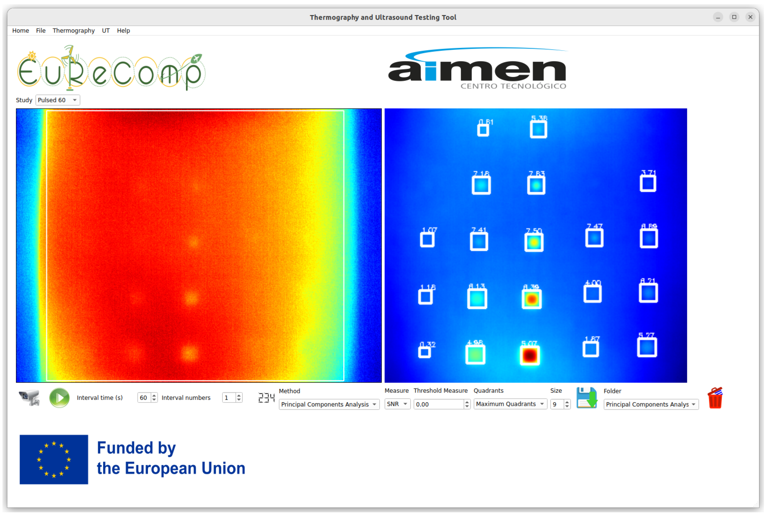
For both image capture and subsequent post-precessing with PPT and PCT, we used the Thermogarphy and Ultrasound Testing Tool (TUTT) available at zenodo.org [15] and developed under the same project as this article.

5. Results and Discussion

The images resulting from the application of PPT and PCT can be seen in Figure 6 and Figure 7, respectively.

In

Table 1. Precision and Recall for methods PPT and PCT.

	PPT	PCT
TP	23	20
FP	7	0
FN	2	5
Total Detections	30	20
Total Defects	25	25
Precision	$0.77$	1
Recall	$0.92$	$0.8$

, True Positives (TP), False Positives (FP), and False Negatives (FN) are specified for both Active Thermography techniques. The PPT method achieves a precision (${\displaystyle \frac{TP}{FP+TP}}$) of $0.77$ and a recall (${\displaystyle \frac{TP}{TP+FN}}$) of $0.92$. The PCT method achieves a precision of 1 and a recall of $0.8$.

On the other hand, in

Table 2. SNR value for each defect for methods PPT and PCT. Detections are in green, and non-detections are in red.

Defect ID	PPT	PCT
D1	$5.45$	$5.27$
D2	$5.18$	$1.87$
D3	$5.89$	$5.07$
D4	$4.88$	$4.96$
D5	$4.68$	$0.32$
D6	$6.24$	$6.21$
D7	$5.94$	$4.00$
D8	$4.70$	$6.39$
D9	$5.47$	$6.13$
D10	$5.00$	$1.18$
D11	$6.41$	$6.59$
D12	$5.30$	$7.47$
D13	$1.24$	$7.50$
D14	$6.31$	$7.41$
D15	$5.09$	$1.07$
D16	$5.27$	$3.71$
D17	$2.04$	$-2.83$
D18	$1.74$	$7.63$
D19	$6.37$	$7.16$
D20	$2.53$	$-2.38$
D21	$1.33$	$-9.83$
D22	$-5.48$	$-15.03$
D23	$0.63$	$5.36$
D24	$4.03$	$0.61$
D25	$-4.29$	$-10.88$

, the SNR for all defects can be seen.

Comparing both techniques, in other tests, it can be seen that, while PPT obtains a better recall, i.e., it effectively detects more defects, PCT obtains a better precision, i.e., it detects fewer fake defects in proportion with the total real defects.

6. Conclusions and Future Works

In this work, pulsed thermography was applied to a GFRP calibration plate with the aim to detect half hole defects. The concepts of PPT and PCT have been reviewed for the processing and analysis of thermal images. Each signal processing technique was evaluated by the automatic use of SNR. Based on the results, it was determined that the automatic use of SNR is highly effective when defects are larger than 5 mm in diameter. However, when defects are less than 5 mm in diameter and less than 2.5 mm deep, the method should be improved.

Comparing PPT and PCT, it could be observed that PPT performs better in finding smaller and deeper defects, while PCT provides a higher SNR on larger defects closer to the surface. On the other hand, PPT tends to make more errors in detection than PCT, thus obtaining a higher precision for the latter method.

Future work will focus on applying these methods in real scenarios, such as the inspection of a wind turbine blade, and improving their implementation.

References

- Sathishkumar, T.; Satheeshkumar, S.; Naveen, J. Glass fiber-reinforced polymer composites—A review. J. Reinf. Plast. Compos. 2014, 33, 1258–1275. [Google Scholar] [CrossRef]
- Chen, J.; Yu, Z.; Jin, H. Nondestructive testing and evaluation techniques of defects in fiber-reinforced polymer composites: A review. Front. Mater. 2022, 9, 986645. [Google Scholar] [CrossRef]
- Usamentiaga, R.; Venegas, P.; Guerediaga, J.; Vega, L.; Molleda, J.; Bulnes, F.G. Infrared Thermography for Temperature Measurement and Non-Destructive Testing. Sensors 2014, 14, 12305–12348. [Google Scholar] [CrossRef] [PubMed]
- Parker, W.; Jenkins, R.; Butler, C.; Abbott, G. Flash method of determining thermal diffusivity, heat capacity, and thermal conductivity. J. Appl. Phys. 1961, 32, 1679–1684. [Google Scholar] [CrossRef]
- Wang, R.; Pei, C.; Xia, R.; Wang, Q.; Chen, Z. A portable fiber laser thermography system with beam homogenizing for CFRP inspection. NDT E Int. 2021, 124, 102550. [Google Scholar] [CrossRef]
- Chung, Y.; Lee, S.; Kim, W. Latest advances in common signal processing of pulsed thermography for enhanced detectability: A review. Appl. Sci. 2021, 11, 12168. [Google Scholar] [CrossRef]
- Maldague, X. Theory and Practice of Infrared Technology for Nondestructive Testing; Wiley-Interscience: Hoboken, NJ, USA, 2001. [Google Scholar]
- Maldague, X.; Galmiche, F.; Ziadi, A. Advances in pulsed phase thermography. Infrared Phys. Technol. 2002, 43, 175–181. [Google Scholar] [CrossRef]
- Pearson, K. Principal components analysis. Lond. Edinb. Dublin Philos. Mag. J. Sci. 1901, 6, 559. [Google Scholar] [CrossRef]
- Daultrey, S. Principal Components Analysis; Geo Abstracts Limited: Norwich, UK, 1976; Volume 8. [Google Scholar]
- Rajic, N. Principal component thermography for flaw contrast enhancement and flaw depth characterisation in composite structures. Compos. Struct. 2002, 58, 521–528. [Google Scholar] [CrossRef]
- Milovanović, B.; Gaši, M.; Gumbarević, S. Principal component thermography for defect detection in concrete. Sensors 2020, 20, 3891. [Google Scholar] [CrossRef] [PubMed]
- Gragido, W.; Pirc, J.; Selby, N.; Molina, D. Chapter 4—Signal-to-Noise Ratio. In Blackhatonomics; Gragido, W., Pirc, J., Selby, N., Molina, D., Eds.; Syngress: Boston, MA, USA, 2013; pp. 45–55. [Google Scholar] [CrossRef]
- InfraTec GmbH Infrarotsensorik und Messtechnik. InfraRed Camera VarioCAM HD Head 800. Available online: https://www.infratec.eu/thermography/infrared-camera/variocam-hd-head-800/ (accessed on 28 October 2024).
- Asociación de Investigación Metalúrgica del Noroeste; Fernández, M.G.; Boga, D.C. Thermography and Ultrasound Testing Tool. 2024. Available online: https://doi.org/10.5281/zenodo.13833956 (accessed on 28 October 2024).