Permanent Train-Side GNSS Multipath Characterization Considering Time-Correlation for Safe Railway Localization ^†

Abstract

Railway transportation systems have high accuracy and high integrity demands for safe localization. In the future, railway signaling is expected to rely on onboard sensors like Global Navigation Satellite Systems (GNSSs) in order to reduce installation and maintenance costs. GNSS position determination can, however, be highly degraded because of the presence of multipath on the train and railway environment. This paper tackles the characterization of multipath in code measurements caused exclusively by the antenna installation and derives a conservative error model of the antenna-installation-induced multipath and noise. First, we isolate multipath and noise from other GNSS errors using the Code-Minus-Carrier method. Second, an overbounding error model is derived. The limitation of modeling with restricted set of real data typically found in practice is discussed and we review methods that ensure the independence of samples. A new approach that creates separate data sets is ultimately proposed to derive an overbounding sigma. The presented methodology is supported by real measurements collected in an open-sky railway scenario. The derived models can be used as a reference nominal error models to build the null hypothesis of fault detection algorithms that detects the presence of excessive multipath in dynamic scenarios or as a part of a total error budget consideration.

1. Introduction

Recent developments in railway localization systems have targeted replacing track-side based signaling systems, such as balises, with an on-board based localization solution. Most of the on-board localization system proposals have leaned towards implementing a fusion solution of different sensors, with Global Navigation Satellite Systems (GNSSs) playing a key role. The use of GNSSs can potentially reduce the installation and maintenance costs of infrastructure-based signaling systems compared to infrastructure ones while, at the same time, ensuring cross-country interoperable safe operations. However, GNSS positioning can be challenging in railway environments because GNSS signals can be highly affected by multiple reflections (i.e., multipath) and other GNSS threats like non-line-of-sight (NLOS) signals or the presence of interference. Multipath is particularly pronounced on trains due to the presence of multiple irregular metal elements on the roof and the limitation of optimal antenna placement locations. Moreover, the complex and dynamic nature of the railway surroundings makes predicting and mitigating multipath effects particularly challenging.

Research and development efforts to overcome these challenges have led to a range of solutions across different stages of GNSS receiver processing, for example, at the hardware- or correlator-signal-processing level. For safety-related applications, error characterization is typically performed at post-correlation level [1,2].

Modeling multipath at this stage is a cost-effective solution, that can be performed with commercial off-the-shelf antennas and receivers, avoiding the need for complex and expensive hardware solutions.

The detection and estimation of multipath relies on statistical knowledge and assumptions about the error. It is, however, challenging to isolate and characterize multipath in land-based applications due to the varying nature of the measurements [3].

Multipath error caused by the surrounding operational environment is expected to be changing during the train’s movement, while multipath caused by the vehicle structure and antenna installation is expected to have similar stochastic properties for a given satellite elevation and azimuth with respect to the user. This permanent multipath contribution is assumed in this work to be the basis for constructing error models and fault detectors for the operational environment, and it will be the focus in this paper.

In order to meet the high integrity requirements needed for safety-critical applications, GNSS multipath errors must be properly characterized. Robust error modeling has been achieved in other applications by the Gaussian overbounding method [4]. In this method, the unknown true error distribution is replaced by a Gaussian distribution, which preserves its bounding properties after convolution in the position domain. This theorem has been extended in [5]. Error model bounds considering the correlation of samples have previously been tackled in [1,6]. In previous work, a first approach to model the antenna-installation-induced multipath and noise for trains was introduced [7]. However, the models were derived without considering the time correlation of the collected sample data.

In this paper, we extend the work in [7] and derive robust code multipath error models for the permanent multipath error, e.g., the contribution due to antenna installation and surrounding train rooftop. The methodology takes into account the limitation of the number of sample data typically found in practice. We also propose a new approach to use all the available data when determining overbounding distributions by evaluating different sets of independent samples.

Models are obtained for different train installations with real data collected during the EU ERSAT-GCC project.

2. Multipath Error Modeling Methodology

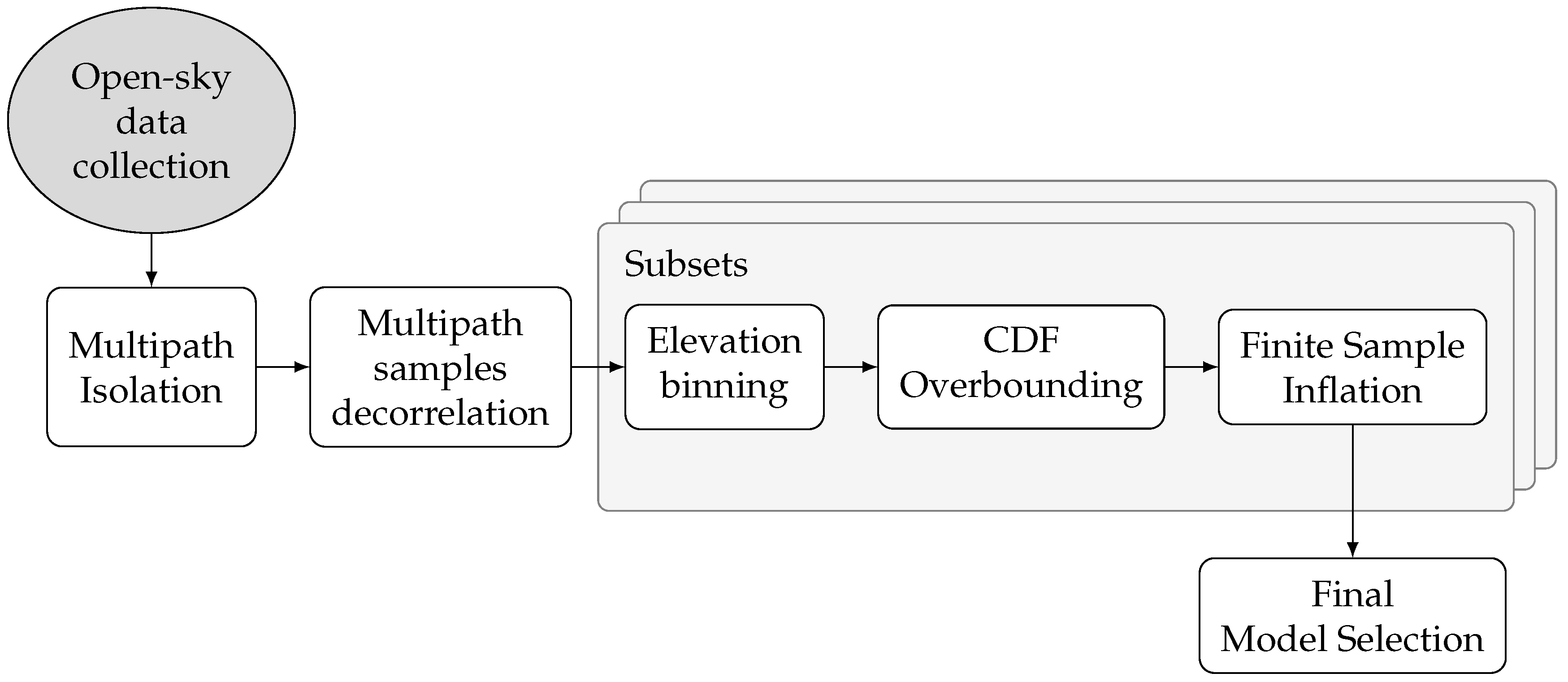
Since permanent multipath error estimates are expected to have high levels of time correlation, we propose the following methodology in order to derive permanent multipath error models based on independent samples. Figure 1 gives a graphic overview of different methodology steps. The first step is the collection of the appropriate dataset for the implementation of the methodology, which is in this case a long, static, and open-sky scenario dataset. The second step is the isolation of the permanent train code measurement multipath error with the Code-Minus-Carrier method, followed by the decorrelation of the multipath samples. The next steps are repeated separately for each of the created subsets of independent samples. Those steps are, firstly, elevation-dependent binning, since multipath errors are highly elevation dependent, and secondly, calculating the CDF overbound for every elevation bin. The last step performed for every subset is the finite sample inflation to account for the limited number of samples available. Lastly, the final step of the proposed methodology is selecting the final overbounding model.

2.1. Open-Sky Data Collection and Multipath Isolation

In order to model the permanent multipath behavior, it is first necessary to obtain GNSS measurements that are not affected by the varying multipath observed during railway-along-track operations. This can be done by collecting data in static, open-sky scenarios during longer periods of time, as suggested in [7]. By collecting data in this way, we try to minimize the contribution of the varying multipath errors. In other words, we presume that the total isolated multipath error is the permanent train multipath error caused by the antenna installation. Multipath is isolated by using the Code-Minus-Carrier (CMC) observable [8].

Code-Minus-Carrier (CMC) is expressed as a difference of pseudorange measurements ${\rho }_k^s$ and corresponding carrier phase measurements ${\varphi }_k^s$ for satellite s at time k. As shown in [3], for a single receiver, satellite s and frequency j can be expressed as follows:

$$CM{C}_k^s={\rho }_k^s-{\varphi }_k^s=M{P}_k^s+(2I_k^s-\lambda N_k^s)+({\epsilon }_k^s-m{p}_k^s-{\xi }_k^s),$$

(1)

where $M{P}_k^{s,j}$ and $m{p}_k^{s,j}$ are the multipath errors of code and carrier phase measurements, $I_k^{s,j}$ represents ionospheric error, $N_k^{s,j}$ denotes carrier phase integer ambiguities (in cycles), ${\lambda }_j$ corresponds to the wavelength, and ${\epsilon }_k^{s,j}$ and ${\xi }_k^{s,j}$ represent code and phase noise, respectively. The CMC combination eliminates all common errors terms. However, it retains code multipath errors, carrier-phase multipath errors, code and carrier-phase noise, carrier-phase ambiguities, as well as twice the ionospheric delay. Assuming that carrier-phase multipath and noise are significantly smaller in magnitude compared to code multipath and noise, they can be neglected.

The ionospheric error can be estimated and removed by a linear combination of two carrier-phase measurements received for the same satellite at the same time epoch [1]. The resulting linear combination of carrier-phase ambiguities can be eliminated by leveraging the fact that integer ambiguities remain constant during a continuously tracked cycle-slip-free period [3], allowing for bias estimation and removal.

2.2. Multipath Samples Decorrelation

Multipath errors are expected to be correlated over time due to the presence of elements in the surrounding of the antenna and the relative slow movement of satellites with respect to the user LOS. However, estimating the variance based on correlated samples would lead to a biased estimation, as seen, for example, in [9]. For that reason, it is necessary to consider only decorrelated samples when deriving parameters of sample distributions in our case of a multipath error model.

In this work, the construction of empirical distributions is based on samples that are separated by at least their correlation time. One possibility for determining the correlation time is to investigate the autocorrelation of every time series.

The level of time correlation of a signal can be studied by the autocorrelation function, which can be expressed, based on the expectation operator, as follows [10]:

$${\overline{R}}_{\widehat{\mathit{MP}}}(\Delta t)={\displaystyle \frac{E\left[{\widehat{\mathit{MP}}}_0{\widehat{\mathit{MP}}}_{\Delta t}\right]-E{\left[\widehat{\mathit{MP}}\right]}^2}{{\sigma }_{\widehat{\mathit{MP}}}^2}}.$$

(2)

where ${\sigma }_{\widehat{\mathit{MP}}}^2$ is the variance of the signal and E is the expectation operator.

Analyzing the autocorrelation of the different time series of the isolated multipath for all satellites allows us to estimate a minimum necessary time lag between two data samples in order to be considered independent.

The necessary time lag is estimated by finding the time lag for which their normalized autocorrelation is within a threshold of $\pm 0.2$, since $0.2$ is typically in statistics considered as the limit for weak correlation [1]. In the remaining paper, the median time lag of all normalized autocorrelations is used to select decorrelated samples to derive multipath models.

Creating one independent dataset by selecting single samples separated by the estimated decorrelation time lag significantly reduces the amount of available data. Moreover, it does not guarantee that this specific subset contains possible outliers.

For that reason, we did not create a single subset of independent samples, but we created all possible subsets with independent samples. More specifically, if $a=t_c{f}_s$ is the estimated decorrelation time lag, where $t_c$ is the average time correlation constant of the processes and $f_s$ is the sampling frequency, we define the subset index k such that $k=1,2,\dots a$ and $k\in \mathbb{N}$. The subset ${\mathbf{z}}_k$ is defined as selected multipath estimates for all satellites in view and given epochs such as

$$\begin{array}{c}{\mathbf{z}}_k:=\left\{{\widehat{\mathit{MP}}}_{\rho }\left(t_{k+(i-1)a}\right)\right\};\hspace{1em}\forall i=1,2,\dots ,{\displaystyle \frac{M}{a}};\hspace{1em}{\displaystyle \frac{M}{a}}\in \mathbb{N},\end{array}$$

(3)

where M is the number of all samples collected.

By adopting this systematic approach, we can analyze and compare the properties across various sets of independent samples and avoid the possibility of analyzing a single dataset which might not be representative of the expected errors but allows for gaining a comprehensive understanding of their distinct characteristics.

As an illustrative example of the subsets selection, Figure 2 is provided.

According to Equation (3), in Figure 2, ${\widehat{\mathit{MP}}}_{\rho }$ represents the sample dataset, and ${\mathbf{z}}_k$ represents the four subsets of independent samples.

2.3. Elevation Binning, CDF Overbounding, and Sample Inflation of a Subset Dataset

However, if $X_1,X_2,\dots X_n$ are observations of size n from a normal distribution $N(\mu ,{\sigma }^2)$. If $\overline{X}$ is a sample mean of n observations, and $S^2$ is the sample variance. Then it follows that the variance is chi-squared distributed since:

$${\displaystyle \frac{(n-1)S^2}{{\sigma }^2}}={\displaystyle \frac{{\sum }_{i=1}^n{(X_i-\stackrel{-}{X})}^2}{{\sigma }^2}}\sim {\chi }^2(n-1).$$

(4)

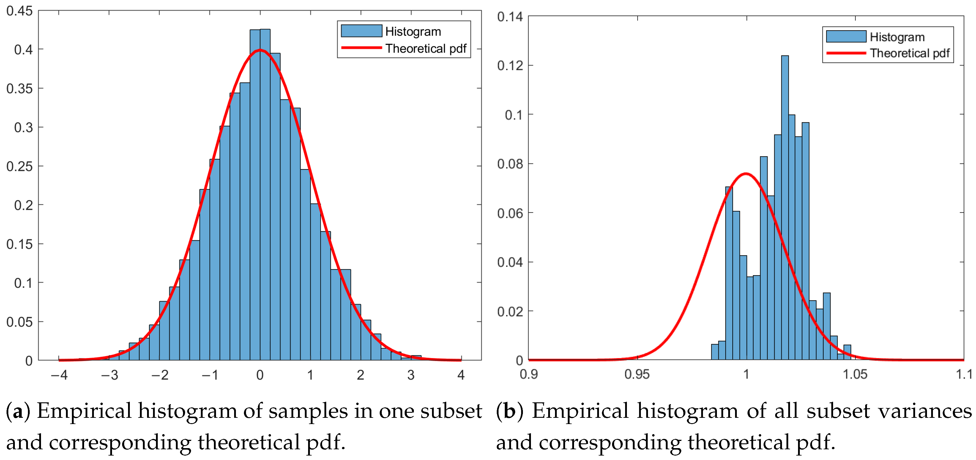
Figure 3 is given as an illustrative example of the impact of correlation. The derivation of sets of independent samples, as presented in Equation (3), can be simulated by a sequence of Monte Carlo simulations and a first-order Gauss–Markov process ($GM({\sigma }^2,\tau )$). The subsets created are indeed comprised of independent samples, as seen in Figure 3a. In Figure 3a, it can be seen that the sample distribution follows a theoretical probability density function of a normal distribution. However, since the subsets originate from a dataset which is comprised of correlated samples, the computed variances of subsets of independent samples remain correlated, as seen in Figure 3b. The variance distribution in Figure 3b does not follow the theoretical probability density function of a chi-squared distribution, as would be expected following Equation (4).

After creating all the subsets of independent samples, the remaining methodology steps are defined for each subset of independent samples separately. First, the elevation binning is performed. The satellite signal reflection depends on the elevation angle between the satellite and the user; hence, the multipath error is expected to highly depend on the elevation angle [7]. The decorrelated multipath sample estimates from all satellites are grouped by their elevation angle. The elevation bin width is adjusted to balance a similar minimum number of samples in each elevation bin.

As a next step, our goal is to determine a parametric distribution based on the samples in each elevation bin. Since, in a general sense, the samples do not follow a Gaussian distribution, and, in most cases, they show longer tails [1], a Gaussian overbounding process is used instead of a simple variance estimator.

In particular, the overbounding methodology, according to [5], involves determining the likely error distribution by collecting a sample distribution. According to [11], the most common choice for this simpler, likely error distribution is the normal distribution, as it is the only finite variance distribution that remains stable through convolution. For that reason, it is assumed that overbounding can be achieved by employing the Cumulative Density Function (CDF). Furthermore, the [5] approach separately calculates the left-hand and right-hand sides of the CDF. What is obtained for each of the subset of independent samples and each elevation bin is both the overbounding sigma estimate and a bias.

Finally, since ensuring independent samples, i.e., dividing the data into subsets, and further dividing it into elevation bins may reduce the number of available samples for each elevation bin, an inflation factor is applied to the variance to account for the finite samples, similarly to [1]. The inflation factor $K_i$ of the measurements-based standard deviations with respect to the truth is determined based on the chi-square distribution of the variance as follows:

$$K_i=\sqrt{{\displaystyle \frac{H-1}{B}}}.$$

(5)

where H represents the number of effective independent samples utilized in deriving the variance for each elevation bin. Thus, in our case $H=H_{min}$, B is defined as the value at which the chi-square distribution ${\chi }_H^2-1$ achieves a probability of $1-\alpha$ (for a $95\%$ confidence interval, $\alpha =0.05$). This formula is chosen based on the principle that the variance estimate obtained from a finite sample size is, in fact, a random variable that follows a chi-squared distribution with H-1 degrees of freedom. In this case, we use the CDF overbounding methodology to account for the non-Gaussianity of the sample dataset, while the inflation factor is used to account for the limited number of samples.

It can be shown that, from around 300 samples, the necessary inflation factor to guarantee $95\%$ estimation probability is close to one. We have used this value to guarantee the minimum number of samples available in each bin.

2.4. Final Model Selection

The last step of the methodology is the final model selection. The final model selection is performed after creating all separate datasets that contain independent samples, determining the overbounding sigma and inflating the overbounding sigma estimate to account for the limited number of samples, as introduced in Equation (5).

Two possibilities for a final model selection are introduced. The final model can be selected based on the $95\%$ quantile of the estimated inflated sigma CDF overbound of all subsets or based on the median of the estimated inflated subset sigma CDF overbound of all subsets. Selecting the $95\%$ quantile would allow for a more conservative error model of the isolated multipath, while selecting the median as a final model would provide a tighter bound. In the future, we will investigate the better suitability of one of the two options, depending on the specific application and goal.

3. Experimental Setup

Results presented in this paper are obtained based on data collected within the European Union ERSAT-GGC project. The dataset was collected during a measurement campaign in Cagliari, Italy, in open-sky and static conditions during the course of eight consecutive hours. The location of the train during the data recording is shown in Figure 4. The setup consisted of a commercial train ALn668-3136 from Trenitalia. The GNSS antenna installed on the train was Antcom G5 antenna, and it was internally connected with a Javad Delta-3N receiver. The receiver was collecting raw measurements with a sampling rate of 10 Hz.

During the collection of the data, the train was placed an as close as possible to an open-sky scenario, given the operational constraints. This allowed for the isolated multipath error to be considered as the multipath caused exclusively by the antenna installation. Furthermore, the long-term recording enables the assumption that the integer ambiguities of the carrier-phase measurement can be successfully estimated and removed (as introduced in Section 2.1). Additionally, we can obtain measurements from a variety of different elevation angles and azimuths.

4. Results

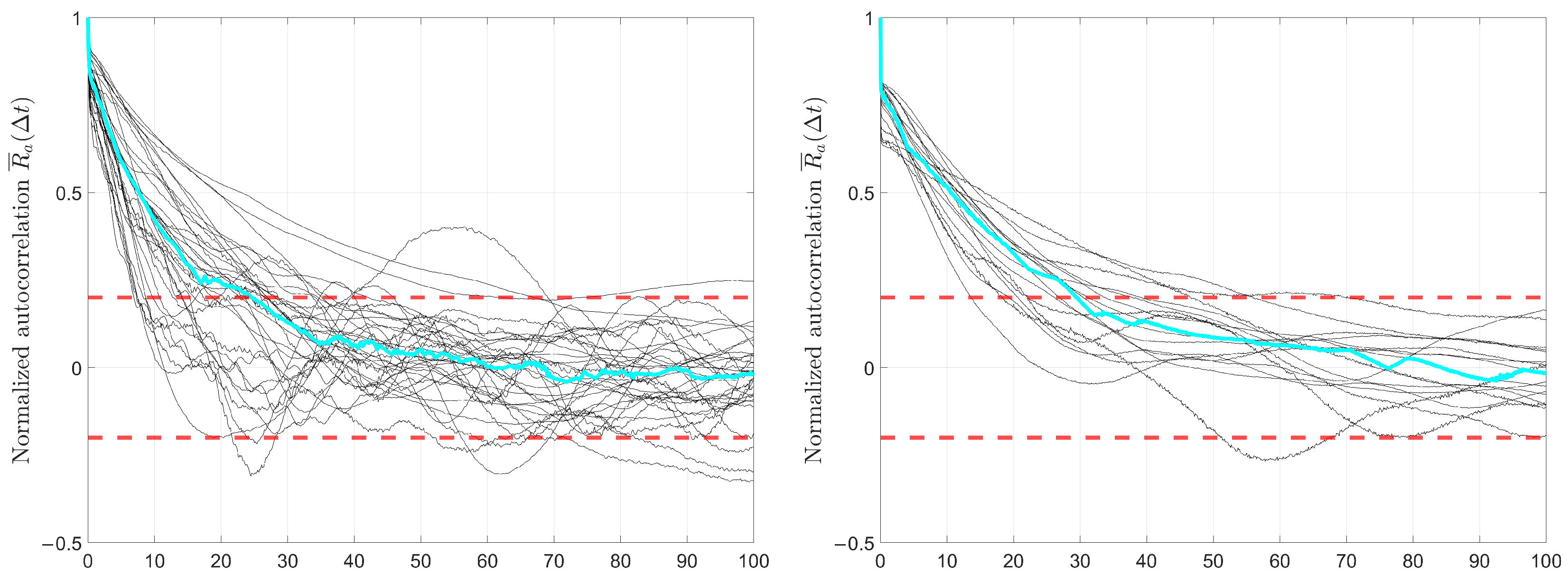
Following the methodology steps introduced before, we first isolate the code multipath of the measured GNSS signals and, second, derive the time lag of the correlated multipath estimates. The result of time lag estimation based on the normalized autocorrelation for the ERSAT-GGC data set is given in Figure 5.

The time lag used for the decorrelation of the samples is the mean time lag based on the normalized autocorrelation of all available time series and equals, in this case 25 s for GPS L1 and 29 s for Galileo E1 measurements.

Following that, we generated the different subsets, each containing only independent samples. The multipath estimates of each subset are separated into different elevation bins, such that in each elevation bin, we do have the minimum number of 300 samples. This resulted in 19 elevation bins for both GPS and Galileo.

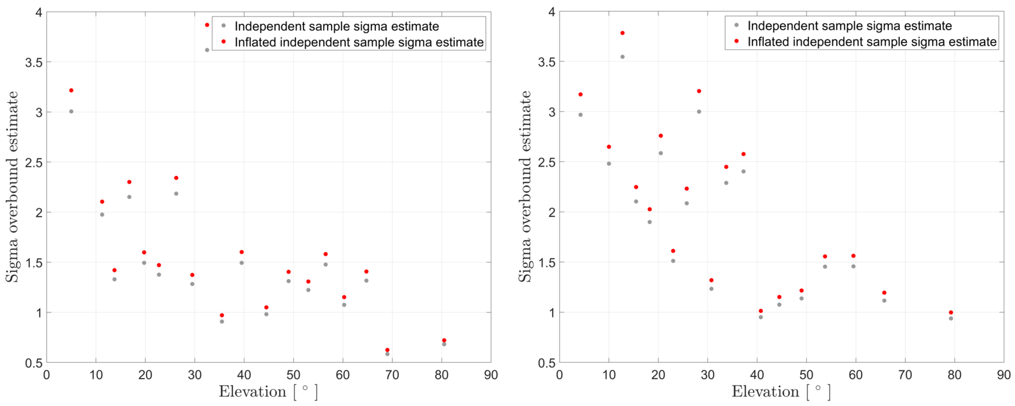
Next, we calculate the CDF overbound, resulting in a left and right hand bias and sigma estimate, we consider only the maximum of both estimates. Finally, we inflated this sigma estimate to account for the limited number of samples. The results are given in Figure 6.

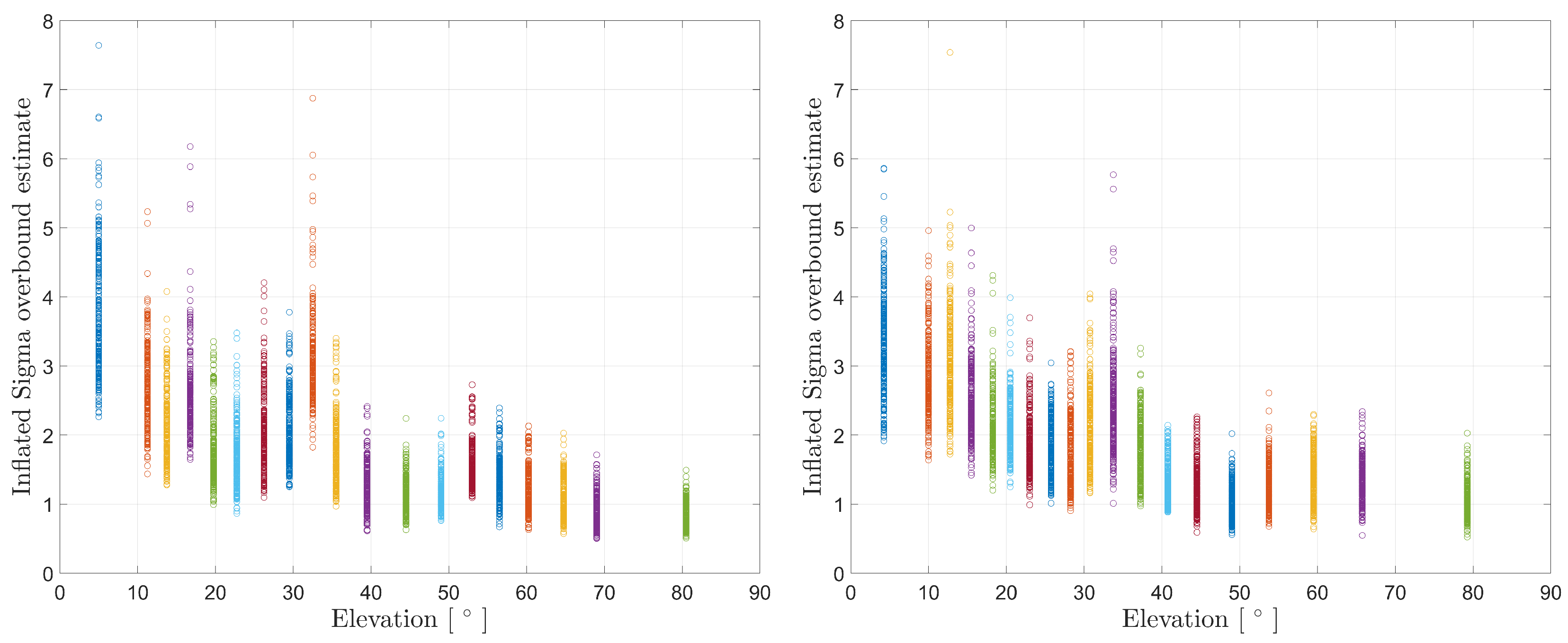
As introduced, we calculated the CDF overbound of every subset containing independent multipath estimates. We repeated the CDF overbound and the finite sample inflation for all generated data subsets of independent samples. The corresponding sigma estimates are shown in Figure 7. Figure 7 shows sigma values of different independent subsets, colored according to the corresponding elevation bins. In other words, different colors denote sigmas of different elevation bins. Each sigma estimate was inflated with the exact inflation factor based on the number of samples in the corresponding elevation bin.

By computing the overbounding sigmas of all the subsets and inflating them to account for the limited number of samples, and finally providing the model based on only one of the independent subsets, we ensure that the one independent subset is selected after an insight to the full dataset and that the limited number of samples are tackled by adopting the inflation factor.

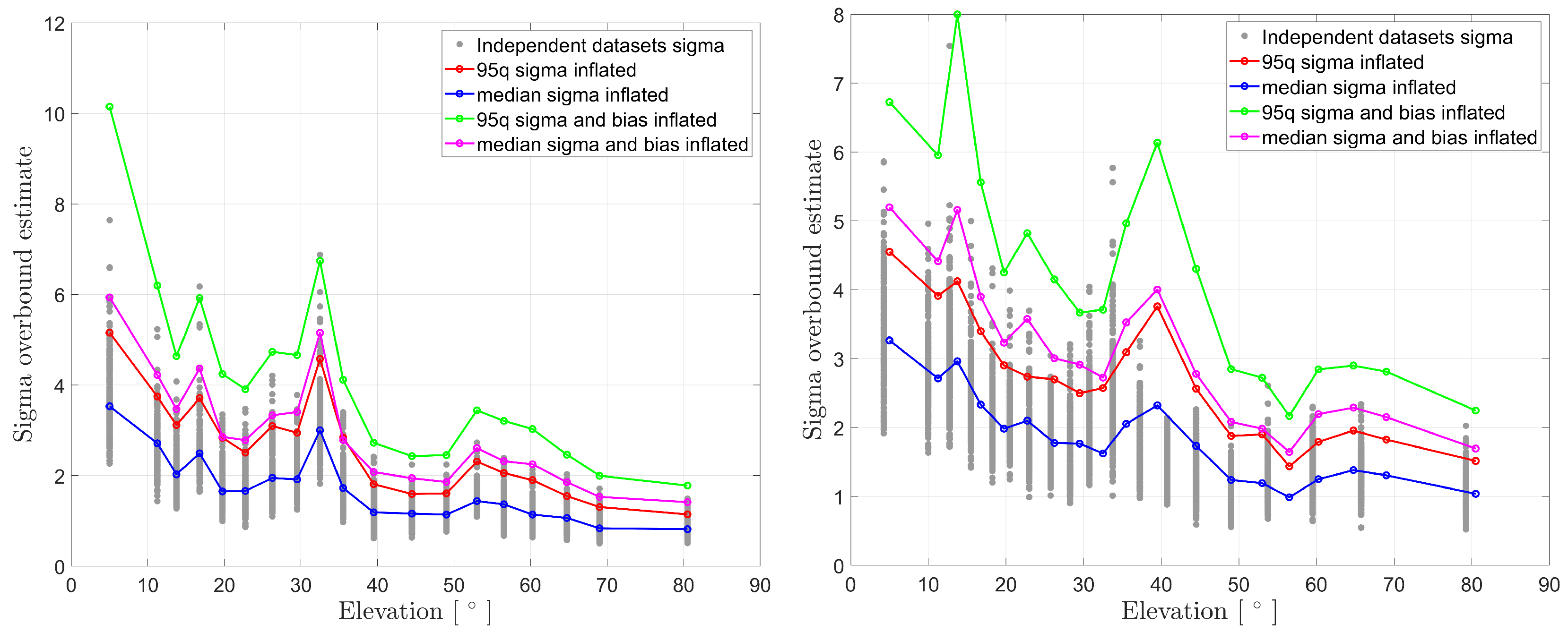
The final step of the methodology is selecting the sigma estimate for the final model selection. Currently, two options are explored: the median inflated sigma estimate and the 95% quantile sigma estimate. The visualization of both is shown in Figure 8.

Finally, since the CDF overbound provides both the sigma estimate and a bias, the models including the bias are given in Figure 9.

5. Conclusions and Future Work

In conclusion, in this paper, we have presented the methodology for a conservative error multipath model, considering time correlation for permanent train GNSS multipath error. Although it is arguable whether physical multipath effect can be decomposed in this way, this allows us to develop a practical methodology to model the total multipath error in post-correlation. In other words, because of the varying nature of multipath, decomposing the total multipath error contribution into two parts allows us to model separate parts of the multipath error, which is otherwise still challenging to model.

The methodology implies gathering static data in open-sky scenarios, assessing sample independence, creating subsets of independent samples, elevation binning and CDF overbounding of every subset of independent samples, and accommodating potential limitations in sample numbers. This reference model is important for deriving fault detection strategies and subsequent models tailored to the railway environment. Nonetheless, it is imperative to acknowledge the operational constraints imposed by this methodology, notably the necessity of collecting specific datasets over extended time periods. For that reason, future work entails deriving guidelines on collecting static measurements for reference multipath error model derivation, most notably its length, as well as further analysis into selecting the overbounding sigma.

References

- Circiu, M.S. Integrity Aspects for Dual-Frequency Dual-Constellation Ground Based Augmentation System (GBAS). Ph.D. Thesis, RWTH Aachen University, Aachen, Germany, 2020. [Google Scholar]
- García Crespillo, O.; Grosch, A.; Adjroloh, P.H.; Zhu, C.; Capua, R.; Frittella, F.; Kutik, O. Multisensor Localization Architecture for High-Accuracy and High-Integrity Land-based Applications. In Proceedings of the 35th International Technical Meeting of the Satellite Division of The Institute of Navigation (ION GNSS+ 2022), Denver, CO, USA, 19–23 September 2022; pp. 1873–1889. [Google Scholar]
- Caamano, M.; García Crespillo, O.; Gerbeth, D.; Grosch, A. Detection of GNSS Multipath with Time-Differenced Code-Minus-Carrier for Land-Based Applications. In Proceedings of the 2020 European Navigation Conference (ENC), Dresden, Germany, 23–24 November 2020. [Google Scholar] [CrossRef]
- Rife, J.; Pullen, S.; Enge, P.; Pervan, B. Paired overbounding for nonideal LAAS and WAAS error distributions. IEEE Trans. Aerosp. Electron. Syst. 2006, 42, 1386–1395. [Google Scholar] [CrossRef]
- Blanch, J.; Walter, T.; Enge, P. Gaussian Bounds of Sample Distributions for Integrity Analysis. IEEE Trans. Aerosp. Electron. Syst. 2019, 55, 1806–1815. [Google Scholar] [CrossRef]
- Perea, S.; Meurer, M.; Pervan, B. Impact of sample correlation on SISRE overbound for ARAIM. Navigation 2020, 67, 197–212. [Google Scholar] [CrossRef]
- Kliman, A.; García Crespillo, O. Characterization of GNSS Multipath in Nominal Open-Sky Scenario for Safe Railway Localization; DGON POSNAV: Berlin, Germany, 2022. [Google Scholar]
- Braasch, M.S. Isolation of GPS Multipath and Receiver Tracking Errors. Navigation 1994, 41, 415–435. [Google Scholar] [CrossRef]
- Box, G.E.; Jenkins, G.M.; Reinsel, G.C.; Ljung, G.M. Time Series Analysis: Forecasting and Control; John Wiley & Sons: Hoboken, NJ, USA, 2015. [Google Scholar]
- García Crespillo, O. GNSS/INS Kalman Filter Integrity Monitoring with Uncertain Time Correlated Error Processes. Ph.D. Thesis, EPFL, Lausanne, Switzerland, 2022. [Google Scholar]
- Blanch, J.; Walter, T.; Enge, P. A Method to Determine Strict Gaussian Bounds of a Sample Distribution. In Proceedings of the ION GNSS, Portland, OR, USA, 25–29 September 2017. [Google Scholar]