Definition of Optimal Ephemeris Parameters for LEO-PNT ^†

Abstract

This paper addresses the selection and justification of ephemeris parameters to be broadcast in a LEO-PNT navigation message. The temporal evolution of LEO orbital elements is analyzed, proving that the GPS/GAL model needs to evolve to cope with LEO orbit dynamics and to ensure high-accuracy ephemeris. In addition, the ephemeris fitting process is performed systematically for different sets of parameters allowing the most convenient parameter combinations to be determined. If adequate parameters are included in an ephemeris model, the fitting error tends to reduce. Beyond ephemeris parametrization, the length of the fitting interval significantly influences the achievable accuracy—for short fitting intervals of 5–10 min with an optimal set of ephemeris parameters, a SISRE at WUL in the order of 1 to 7 mm is obtained.

1. Introduction

Global navigation satellite systems (GNSSs), based on medium Earth orbit (MEO) constellations are currently the only comprehensive technology providing absolute and accurate positioning, navigation, and timing (PNT) services with global coverage. Governments and institutions are showing a growing interest in alternative PNT capacity to improve navigation services and mitigate the risk of disruption in the economy derived from a potential loss of GNSS service. The continuous improvement in space technology that has allowed cost-effective solutions for access to space and the key advantages that low Earth orbits (LEOs) provide for navigation have meant that LEO navigation systems have gained significant attention in recent years as an opportunity to augment and complement existing GNSS systems.

As well as MEO GNSS satellites, LEO navigation satellites broadcast their ephemerides in the navigation message to allow users to efficiently compute the satellites’ coordinates. Ephemerides are a parametrization of the underlying satellite orbits, which must be determined to induce the minimum loss of accuracy with respect to the given orbit. The ephemeris fitting process is extensively and routinely done in GNSS with MEO satellites with a basic set of six Keplerian parameters plus a complementary set of linear-trend-evolution parameters and harmonic terms.

It must be considered that the dynamic conditions for LEO satellites are more complex than for MEO ones. LEOs are particularly influenced by the relevance of higher-order harmonics of the gravitational field and the effects of Earth’s tides and the atmospheric drag. Therefore, although the Global Positioning System (GPS)/Galileo (GAL) ephemeris model is a good starting point, it needs to evolve to cope with LEO orbit dynamics.

This work addresses the selection and justification of parameters to be included in the LEO navigation message, searching for the orbit parametrizations that best fit LEO orbits, paying special attention to the ephemeris fitting error, which is a key factor in meeting the expected accuracy of a few centimeters for LEO-PNT systems.

Research studies on LEO broadcast ephemerides have already been conducted, leading to proposals to incorporate, on top of the GPS/GAL scheme, further linear, quadratic, and harmonic corrective terms to improve the ephemeris accuracy. Based on the temporal variation characteristics of LEO orbit elements, Xie et al. [1] suggested an optimal 20-parameter set to model LEO orbits (adding $C_{rs3}, C_{rc3}, \dot{a}, \dot{n}$ parameters to the GPS/GAL scheme), while Guo et al. [2] proposed a 21-parameter group (adding $\dot{r}, C_{rs1}, C_{rc1}, C_{us3}, C_{uc3}$ parameters), improving the accuracy obtained with the Xie et al. model by 30%.

The methodology followed to obtain the results of this work was inspired by the one presented in these previous research studies. Two software tools have been developed: the first is used to study the temporal evolution of LEO orbital elements, and a second performs the ephemeris fitting process and allows us to identify which combinations of orbital parameters best model LEO orbits.

Nevertheless, this paper embraces a different approach not covered in existing publications. Additional corrective ephemeris parameters that have not been evaluated in previous studies are considered. In addition, the fact that these parameters can become detached from their physical basis when they are numerically adjusted to short fitting intervals is assessed. This characteristic suggests that the potential parameter combinations should not be only selected based on the long-term variation evolution of the orbital elements, but should also be evaluated by systematically performing the fitting process for different sets of parameters. This emphasizes how the fitting interval length and the orbit altitude influence the number of parameters of the optimal model, and highlights the need for different ephemeris models depending on the fitting interval length. This approach leads to optimal ephemeris sets that improve the accuracy of the Guo et al. [2] 21-parameter model by 50%.

2. Analysis of LEO Orbital Elements

The ephemeris parameters used by the GPS [3] and GAL [4], consist of a set of six Keplerian elements (semi-major axis $a$, orbital eccentricity $e$, orbital inclination $i$, right ascension of the ascending node (RAAN) $\Omega$, the argument of perigee $\omega$, and mean anomaly $M$), complemented with corrective terms that model the typical variations of the orbital elements induced by orbit perturbations. These corrective terms are two first-order rates (for RAAN $\dot{\Omega }$ and inclination $\dot{\left(i\right)}$), the mean motion correction parameter $\Delta n$, and six harmonic terms (which modify the argument of latitude $C_{us2}, C_{uc2}$, the inclination $C_{is2}, C_{ic2}$, and the orbital radius $C_{rs2}, C_{rc2}$). These harmonic terms are associated with twice the frequency of the orbital period.

This model is usually referred to as a 16-parameter model, since the 6 Keplerian parameters and the 9 additional evolution parameters are computed for a certain time reference, represented as $t_{0e}$, which completes the model. From these parameters, intermediate quantities such as the mean motion $n$, orbital radius $r$, or the argument of the latitude $u$ are computed, allowing the final computation of the cartesian coordinates of the satellite.

The classical six Keplerian elements are well suited to at least slightly elliptical orbits; however, in the case of near-circular orbits, the difference between the argument of the perigee and the true anomaly disappears and this can cause the fitting algorithm to diverge. For near-circular LEO orbits, the classical Keplerian parameter set needs to evolve to singularity-free Keplerian parameters. The eccentricity, the argument of perigee, and the mean anomaly are substituted by the orbital $x$ and $y$ components of the eccentricity ($e_x$ and $e_y$) and by the mean argument of latitude $\lambda$, obtained following the next relation:

$$e_x=e·\cos \omega , e_y=e·\sin \omega , \lambda =\omega +M.$$

(1)

With singularity-free elements, the parameters that make up the basic 16-parameter set are shown in Table 1:

Table 1. Ephemeris parameters that compose the basic 16-parameter model for near-circular orbits.

Parameter	Definition	Parameter	Definition
$a^{1/2}$	Square root of the semi-major axis	$e_x$	Eccentricity x-component
$e_y$	Eccentricity y-component	$\lambda$	Mean argument of latitude
$i$	Inclination angle	$\Omega$	Right ascension of the ascending node
$\dot{\Omega }$	Right ascension first-order rate	$\dot{\left(i\right)}$	Inclination first-order rate
$\Delta n$	Mean motion difference from computed value	$C_{rs2}, C_{rc2}$	Amplitudes of the 2nd sine and cosine harmonic corrections to the orbital radius *
$C_{us2}, C_{uc2}$	Amplitudes of the 2nd sine and cosine harmonic corrections to the argument of latitude *	$C_{is2}, C_{ic2}$	Amplitudes of the 2nd sine and cosine harmonic corrections to the inclination angle *
$t_{0e}$	Ephemeris reference time

* 2nd harmonic corrections are associated with twice the frequency of the orbital period.

This basic 16-parameter model, although being a good starting point to find the optimal LEO ephemerides, model should evolve to cope with the characteristics of LEO orbits, including further corrective terms. First-order and second-order rates of intermediate orbital elements, and additional harmonic corrections are considered to be potentially included in the navigation message, following the approach promoted in [1,2] but considering further parameters not assessed in these previous studies. Table 2 lays out all the additional corrective terms that have been contemplated.

Table 2. Additional parameters to be potentially included in the LEO navigation message.

Parameter	Definition	Parameter	Definition
$\dot{r}$	Orbital radius first-order rate	$\dot{u}$	Argument of latitude first-order rate
$C_{rs1}, C_{rc1}$	Amplitudes of the 1st sine and cosine harmonic corrections to the orbital radius *	$C_{us1}, C_{uc1}$	Amplitudes of the 1st sine and cosine harmonic corrections to the argument of latitude *
$C_{is1}, C_{ic1}$	Amplitudes of the 1st sine and cosine harmonic corrections to the inclination angle *	$C_{\Omega s1}, C_{\Omega c1}$	Amplitudes of the 1st sine and cosine harmonic corrections to the RAAN *
$C_{\Omega s2}, C_{\Omega c2}$	Amplitudes of the 2nd sine and cosine harmonic corrections to the RAAN	$C_{rs3}, C_{rc3}$	Amplitudes of the 3rd sine and cosine harmonic corrections to the orbital radius **
$C_{us3}, C_{uc3}$	Amplitudes of the 3rd sine and cosine harmonic corrections to the argument of latitude **	$C_{is3}, C_{ic3}$	Amplitudes of the 3rd sine and cosine harmonic corrections to the inclination angle **
$C_{\Omega s3}, C_{\Omega c3}$	Amplitudes of the 3rd sine and cosine harmonic corrections to the RAAN **	$\ddot{r}$	Orbital radius second-order rate
$\ddot{u}$	Argument of latitude second-order rate	$\ddot{\left(i\right)}$	Inclination second-order rate
$\ddot{\Omega }$	Right ascension second-order rate

* 1st harmonic corrections are associated with the same frequency of the orbital period. ** 3rd harmonic corrections are associated with three times the frequency of the orbital period.

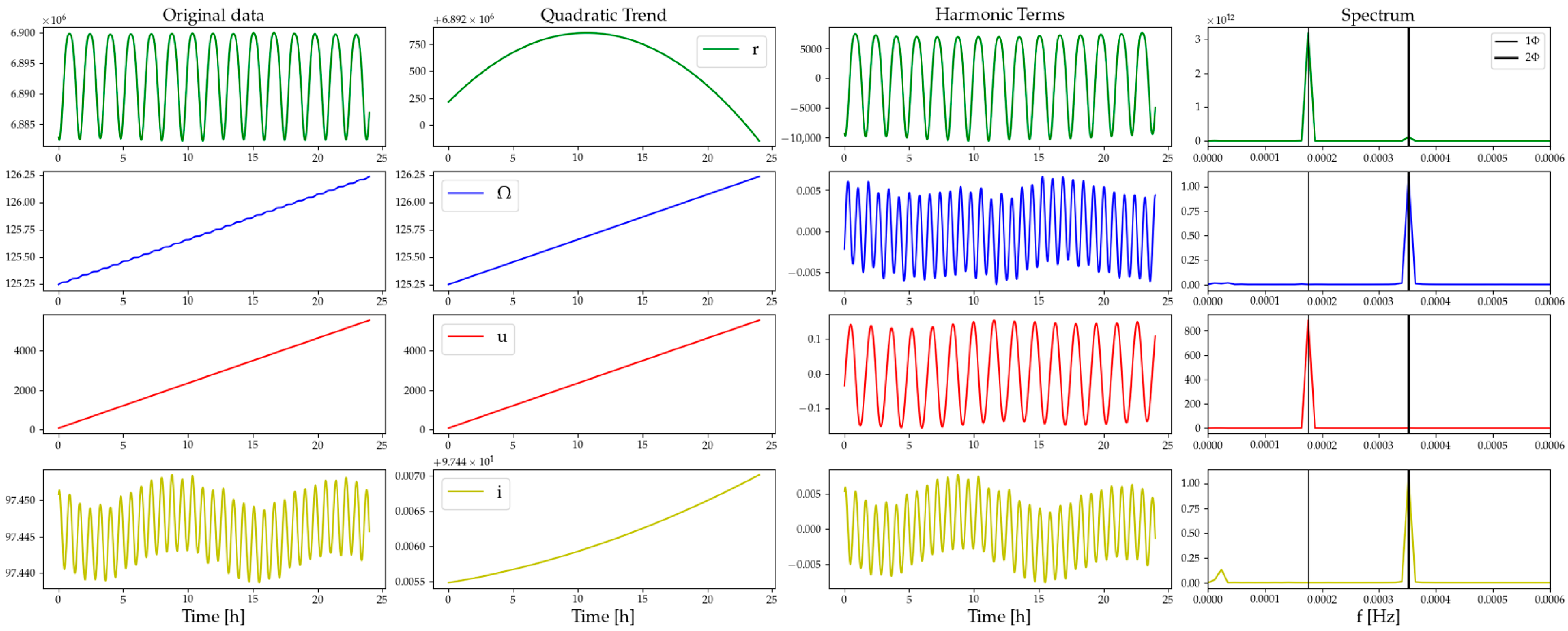
To identify the best representation of LEO orbits, as a first step, the temporal evolution of LEO orbital elements is studied. This study is performed with a software tool that transforms the orbit of a certain satellite into orbital elements, particularly $r$, $\Omega$, $u$, and $i$. To determine which perturbation parameters from Table 2 seem to be more relevant, the long-term quadratic trends and the secular harmonic terms of the evolution of orbital elements are characterized. In addition, Fourier analyses are performed on harmonic terms, showing the most influential harmonic frequencies.

The orbit analyzed in Figure 1 is a 1-day representative LEO orbit with an approximate altitude of 510 km. A low altitude orbit has been intentionally selected, as a worst case, as it has been observed that orbital perturbations gain a greater relevance in the orbital dynamics the lower the altitude is. This orbit is obtained with MAORI, a Flight Dynamics and Geodesy library developed at GMV [5], with the force models of Table 3.

Figure 1. Temporal evolution of orbital elements of the reference 510 km altitude LEO orbit.

Table 3. Orbit modeling used for LEO-PNT simulated orbit.

Force Model	Value	Force Model	Value
Gravity field	EIGEN.GRGS.RL04 TVG (100 × 100), drift/annual/semi-annual linear terms up to 90 × 90.	Ocean tides	FES2014 (100 × 100, 100 tidal constituents)
Solid Earth tides	IERS 2010	Earth and ocean pole tides	IERS 2010
Relativity	IERS 2010	Third bodies	Sun, moon, planets DE-421
Atmospheric density model	msise00	Drag coefficient	Fixed to 2.0

From Figure 1, it can be concluded that parameters $r$ and $u$ show harmonic terms with the same frequency as the orbit, while $\Omega$ and $i$ parameters present terms associated with twice the frequency of the orbit. For long-orbit periods, the harmonic analysis shows that, in addition to the GPS/GAL 16-parameter set, it is essential to consider $\dot{r}$, $\ddot{r}$, $\dot{u}$, $\ddot{\left(i\right)}$, $C_{rs1}, C_{rc1}$, $C_{us1}, \mathrm{and} C_{uc1}$ parameters in order to achieve a high-accuracy ephemeris model.

Nevertheless, it must be highlighted that, if short orbit intervals are analyzed, the difference between the long-term evolution and the short-term secular variations becomes diffuse, and when numerically adjusting ephemeris parameters some parameters can absorb the physical effect corresponding to other parameters and become more relevant. In particular, if ephemerides are fitted to intervals shorter than half the orbital period, the orbital elements that have a harmonic variation with the same frequency of the orbital period can be clearly modeled with a parabolic evolution, and the second-order rate parameter acquires the physical correspondence of the harmonic variation. Consequently, as will be consolidated in the next section, neither the $\ddot{\Omega }$ parameter nor harmonic corrections with higher frequencies can be discarded.

3. Ephemeris Computation

To find the orbit parametrization that best adjusts to the LEO-PNT satellite orbits, the fitting process of the ephemeris parameters must be performed. A dedicated software tool was developed for the LEO ephemeris computation, designed to conduct optimization analyses, with the capacity to iterate over all correction terms of Table 2 and generate results for all possible combinations between them. To generate these combinations, harmonic terms can only be introduced pairwise, and the second-order rates are only included if the first-order rate of the same parameter is also part of the ephemeris set. This iteration capacity allows us to systematically test all the possible combinations and evaluate the optimal ephemeris parameter set that minimizes the fitting error, not only based on the long-term characteristics of LEO orbital elements, since it was shown in the previous section that some parameters can acquire the physical effect corresponding to others and become more relevant.

3.1. Ephemeris Fitting Algorithm

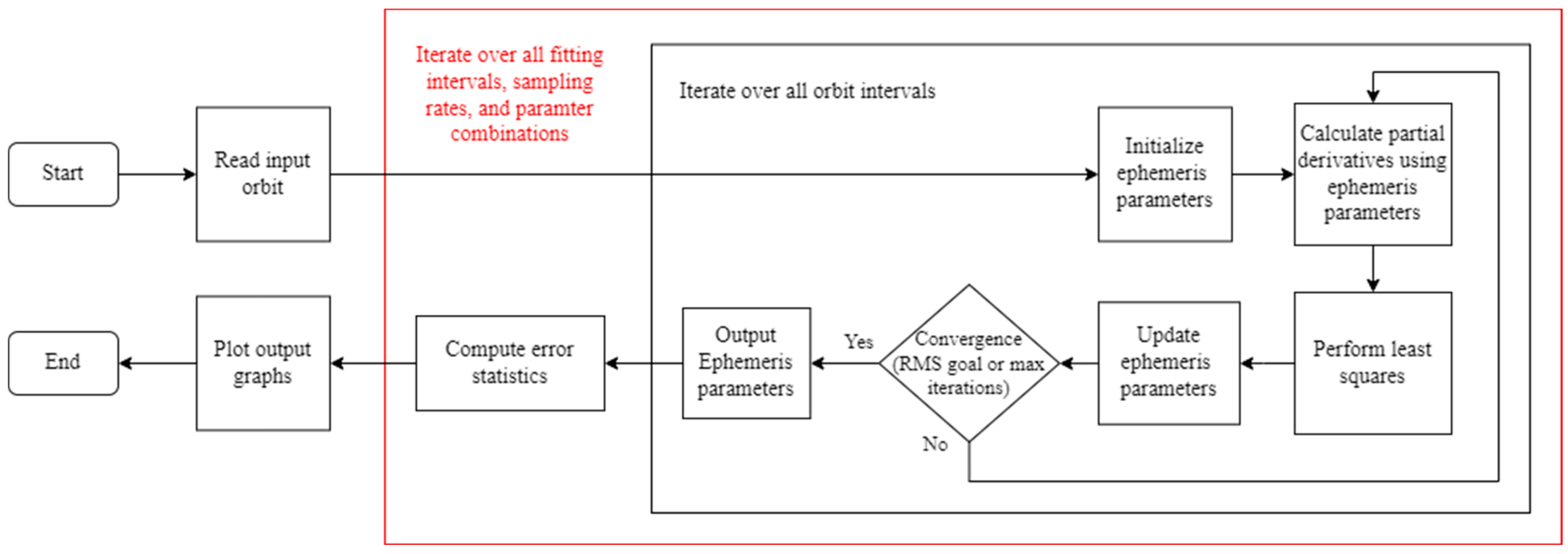
The ephemeris computation tool estimates, via an iterative least square process, the values of the ephemeris parameters that best fit different intervals of the input orbit, for a determined ephemeris parameter set. The input orbit is divided into various intervals, obtaining a new set of ephemeris values for each orbit arc. The length of the fitting intervals and the sampling rate of the orbit points used in the fitting process are both configurable. In addition to all possible parameter combinations, several values of fitting interval length and sampling rate can be included in the same execution of the tool, which allows us to compare how these configuration variables condition the fitting process. The procedure followed by the ephemeris computation tool is illustrated in the scheme of Figure 2.

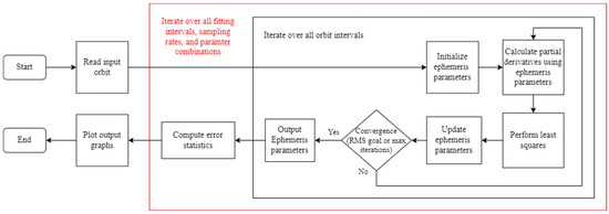
Figure 2. Flow diagram of LEO ephemeris software tool.

In the least squares process, the ephemeris parameters are continuously updated with the variations obtained from the Jacobian matrix and the residuals vector. To avoid ill-posed problems, each column of the Jacobian matrix, which contains the partial derivatives of satellite coordinates with respect to a concrete parameter for all points of the fitting interval, is normalized with its own norm.

The software tool also computes global error statistics regarding all intervals into which the orbit is divided. These error statistics are represented in this work as the signal in space ranging error (SISRE) projected at the worst user location (WUL), considering a masking angle of 5°.

3.2. Results of LEO Optimization Analyses

In the results presented in this section, the 16-parameter model extensively used in GNSS is used as the reference parameter set, meaning that these parameters will always be included in the ephemeris model, adding, on top of them, all possible combinations between the parameters of Table 2.

In addition to the orbit parametrization, the orbit interval length selected to adjust the ephemeris values plays a critical role in the achievable accuracy. Fitting intervals embraced in LEO analyses are considerably shorter than the ones used in traditional GNSS systems. Inversely, the sampling rate selected in the adjustment process demonstrated an insignificant impact on the accuracy obtained. In addition, the orbit altitude also strongly conditions the accuracy obtained, improving the accuracy with the orbit altitude, as detailed in [2], and confirming the accuracy of our ephemeris computation algorithm.

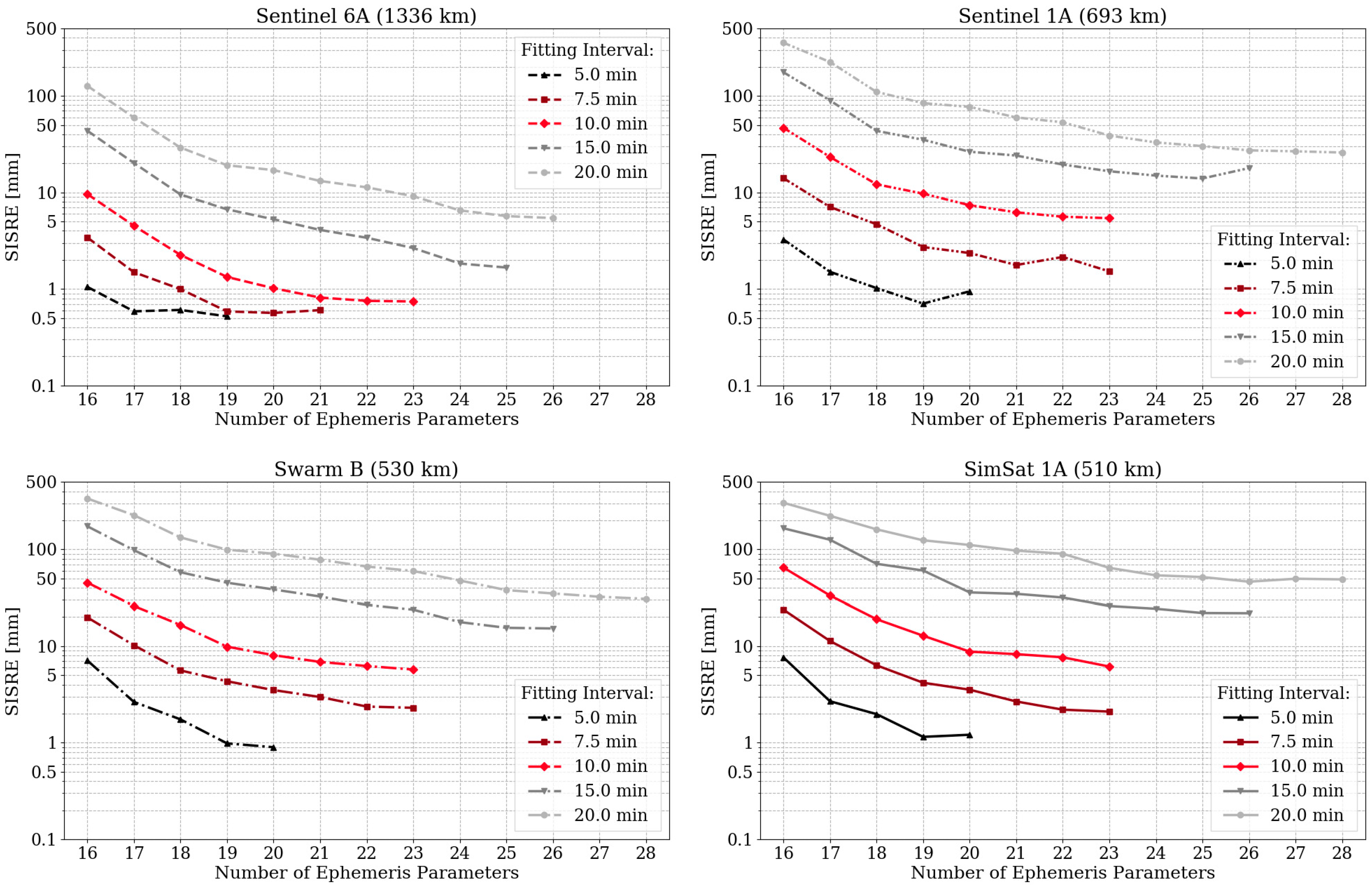
The results of orbits with different altitudes are presented in Figure 3, for various fitting interval lengths ranging from 5 to 20 min. The lowest orbit analyzed is the same satellite orbit as that previously studied, with an approximate altitude of 510 km, obtained with MAORI [5]. It is intentionally selected to examine, in a worst-case scenario, the ephemeris fitting errors obtained. This worst-case analysis, conducted with simulated data, has been supplemented with real data from various satellites, including Sentinel 6A, Sentinel 1A, and Swarm B. Sentinel 1A and Swarm B, both in the lower range of LEO altitudes (693 km and 530 km, respectively), contrast with Sentinel 6A, which operates at a higher altitude (1336 km), representing a best-case scenario. Figure 3 was generated iterating over all possible parameter combinations; however, due to the large number of solutions, only the lowest SISRE from all parameter sets made up of the same number of parameters is represented in the figure for each fitting interval length and satellite.

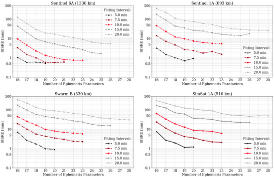
Figure 3. Evolution of SISRE at WUL with the number of parameters that make up the LEO ephemeris model, for various fitting intervals and orbits with different altitudes.

The fitting interval length is the factor with the most influence on the achievable accuracy and on the number of parameters of the ephemeris models that converge through the least squares process. In Figure 3 it can be seen that the longer the fitting interval, the greater the fitting error, even though more solutions with further parameters converge. Solutions with many parameters do not converge for short fitting intervals. However, most accurate solutions are obtained with the shortest intervals, despite the lower number of estimable parameters.

The altitude of the orbit also conditions the fitting error and the ephemeris schemes that converge, improving the accuracy with the orbit altitude. On the other hand, some parameter combinations only converge for the lowest altitudes of the LEO range. The largest parameter combinations do not provide a valid solution for the Sentinel 6A orbit. Despite this, the accuracy obtained with the optimal solution of the Sentinel 6A orbit is greater than the optimal solution of the other orbits analyzed.

For the SimSat 1A orbit and a 10 min fitting interval, a SISRE at WUL well below 1 cm can be achieved, and even close to 1 mm for a fitting interval of 5 min. For the highest Sentinel 6A orbit and a 10 min fitting interval, a SISRE at WUL well below 1 mm is achieved, as well as one very close to 0.5 mm for a 5 min fitting interval. The lowest error values of Figure 3 for each fitting interval length and satellite, with the ephemeris schemes that provide those error values, are shown in Table 4.

Table 4. Parameter combinations that provided the lowest SISRE at WUL values, for various fitting intervals and orbits with different altitudes.

Fitting Interval	No. of Param.	Parameter Combination Added	SISRE [mm]	No. of Param.	Parameter Combination Added	SISRE [mm]
	Sentinel 6A			Sentinel 1A
5 min	19	$C_{rs3} C_{rc3} \ddot{\Omega }$	0.52	19	$C_{rs3} C_{rc3} \ddot{\Omega }$	0.70
7.5 min	20	$\dot{r} C_{rs3} C_{rc3} \ddot{r}$	0.56	23	$C_{us3} C_{uc3} C_{rs3} C_{rc3} C_{\Omega s3} C_{\Omega c3} \ddot{\Omega }$	1.52
10 min	23	$C_{us3} C_{uc3} C_{rs3} C_{rc3} C_{\Omega s3} C_{\Omega c3} \ddot{\Omega }$	0.74	23	$C_{us3} C_{uc3} C_{rs3} C_{rc3} C_{\Omega s3} C_{\Omega c3} \ddot{\Omega }$	5.41
15 min	25	$\dot{r} C_{us3} C_{uc3} C_{us1} C_{uc1} C_{rs3} C_{rc3} C_{\Omega s3} C_{\Omega c3}$	1.67	25	$\dot{r} C_{us3} C_{uc3} C_{us1} C_{uc1} C_{rs3} C_{rc3} C_{\Omega s3} C_{\Omega c3}$	13.95
20 min	26	$\dot{r} C_{us3} C_{uc3} C_{us1} C_{uc1} C_{is1} C_{ic1}{C}_{rs3} C_{rc3} \ddot{\Omega }$	5.43	28	$\dot{r} C_{rs1} C_{rc1} C_{us3} C_{uc3} C_{rs3} C_{rc3} C_{\Omega s3} C_{\Omega c3} \ddot{r} \ddot{\left(i\right)} \ddot{\Omega }$	25.50
	Swarm B			SimSat 1A
5 min	20	$\dot{r} C_{rs3} C_{rc3} \ddot{r}$	0.90	19	$\dot{r} C_{us3} C_{uc3}$	1.15
7.5 min	23	$\dot{r} C_{us3} C_{uc3} C_{rs3} C_{rc3} C_{is3} C_{ic3}$	2.30	23	$C_{rs3} C_{rc3} C_{is3} C_{ic3} C_{\Omega s3} C_{\Omega c3} \ddot{\Omega }$	2.19
10 min	23	$\dot{r} C_{us3} C_{uc3} C_{is3} C_{ic3} \ddot{r} \ddot{\Omega }$	5.73	23	$\dot{r} C_{us3} C_{uc3} C_{is1} C_{ic1} \ddot{r} \ddot{\Omega }$	5.77
15 min	26	$\dot{r} C_{us3} C_{uc3} C_{us1} C_{uc1} C_{rs3} C_{rc3} C_{is3} C_{ic3} \ddot{\left(i\right)}$	15.26	26	$\dot{r} C_{us3} C_{uc3} C_{us1} C_{uc1} C_{rs3} C_{rc3} C_{is3} C_{ic3} \ddot{\Omega }$	21.06
20 min	28	$\dot{r} C_{rs1} C_{rc1} C_{us3} C_{uc3} C_{rs3} C_{rc3} C_{is3} C_{ic3} \ddot{r} \ddot{\left(i\right)} \ddot{\Omega }$	30.73	26	$\dot{r} C_{us3} C_{uc3} C_{\Omega s1} C_{\Omega c1} C_{is1} C_{ic1} C_{rs3} C_{rc3} \ddot{\Omega }$	47.18

It can be seen that the ephemeris parameters that make up the combinations of Table 4 tend to repeat. This indicates that those parameters are the most relevant ones to model short intervals of LEO-PNT orbits. Specifically, harmonic correction terms associated with three times the orbital period acquire a key role in orbit modeling, as the fitting intervals embraced are shorter than the orbital period, as well as $\dot{r}$, $\ddot{r}$, and $\ddot{\Omega }$ parameters. The great relevance of $\ddot{\Omega }$ confirms that perturbation parameters become, in a certain sense, detached from their physical basis when adjusted to short orbit arcs.

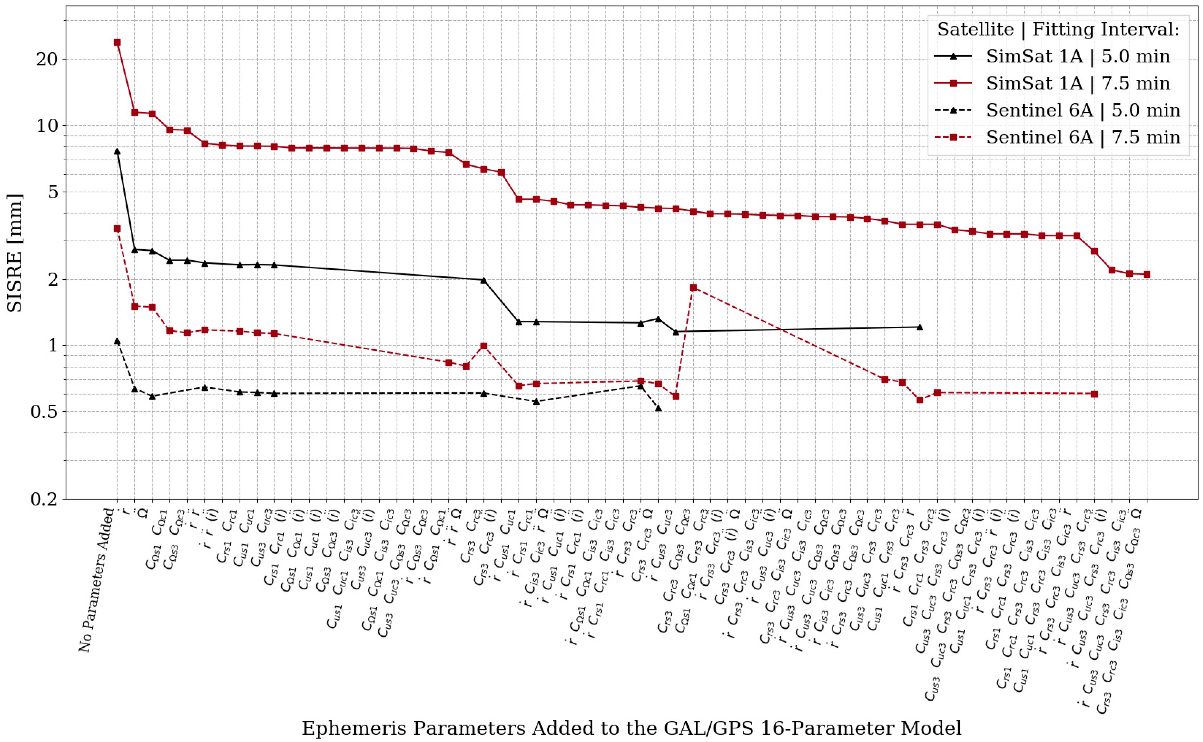
In addition to the parameter sets of Table 4, more parameter combinations converge and provide comparable errors to the minimum for each fitting interval and satellite. Figure 4 illustrates all parameter sets that successfully converge and present a SISIRE at WUL lower than the basic 16-parameter model, for the lowest and highest altitude orbits analyzed, with 5 min and 7.5 min fitting intervals.

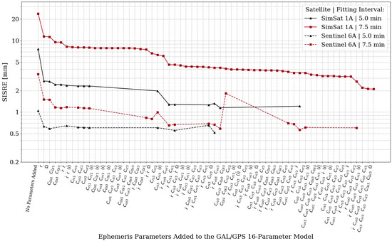
Figure 4. SISRE at WUL provided by all parameter sets subjected to the 16-parameter basic model, for 5 min and 7.5 min fitting intervals and SimSat 1A and Sentinel 6A orbits.

Figure 4 reveals that, in addition to the fact that solutions with a higher number of parameters converge, more combinations with the same total number of parameters can provide a solution as the fitting interval length is increased and the orbit altitude decreases. Also, in addition to the optimal parameter combination for each fitting interval and satellite, more parameter models provide a very similar SISRE at WUL and should be considered as strong candidates to make up a high-accuracy LEO ephemeris model. In particular, the optimal parameter combinations for the Sentinel 6A satellite also provide highly accurate solutions for SimSat 1A, however SimSat 1A optimal combinations are unable to provide a valid solution for the highest orbit.

In the context of potentially standardizing a common ephemeris model for LEO satellites, the model should be adaptable to different altitudes within the LEO regime. Therefore, the optimal ephemeris combinations for Sentinel 6A at each fitting interval length, listed in Table 4, are proposed as the most suitable models, since they can deliver high-accuracy solutions across varying altitudes of the LEO regime. The SISRE at WUL values that they provide for the highest and lowest orbit analyzed are presented in Table 5.

Table 5. Optimal ephemeris models proposed, subjected to the 16-parameter basic parameter set, depending on the fitting interval length.

Fitting Interval Length	Parameter Combination	Approximate SISRE at WUL
		Sentinel 6A	SimSat 1A
20 min	$\dot{r} C_{us3} C_{uc3} C_{us1} C_{uc1} C_{is1} C_{ic1}{C}_{rs3} C_{rc3} \ddot{\Omega }$	5 mm	50 mm
15 min	$\dot{r} C_{us3} C_{uc3} C_{us1} C_{uc1} C_{rs3} C_{rc3} C_{\Omega s3} C_{\Omega c3}$	2 mm	20 mm
10 min	$C_{us3} C_{uc3} C_{rs3} C_{rc3} C_{\Omega s3} C_{\Omega c3} \ddot{\Omega }$	0.7 mm	7 mm
7.5 min	$\dot{r} C_{rs3} C_{rc3} \ddot{r}$	0.6 mm	3.5 mm
5 min	$C_{rs3} C_{rc3} \ddot{\Omega }$	0.5 mm	1.3 mm

The optimal ephemeris models of Table 5 proposed in this paper can be compared with ephemeris schemes of previous research studies. The 21-parameter scheme (adding $\dot{r}, C_{rs1}, C_{rc1}, C_{us3}, C_{uc3}$) selected in [2] provides a SISRE at WUL fitting error in the order of 10 cm with a 20 min fitting interval, around 5 cm with 15 min, and 1.5 cm with a 10 min fitting interval, for orbits higher than 500 km. With the approach of considering different optimal parameter combinations depending on fitting interval and the optimal ephemeris schemes outlined in this paper, the accuracy of the model in [2] is improved by 50% on average. Furthermore, small fitting intervals are also suggested to generate the navigation message, with ephemeris models that provide SISRE values around 3.5 mm for a 7.5 min fitting interval and very close to 1 mm for a 5 min fitting interval.

4. Conclusions

This paper embraces optimization analyses that allow the identification of the ephemeris parameters that best adjust to the LEO satellite orbits and would form the optimal LEO-PNT ephemeris model to be included in the navigation message. The analysis of the temporal evolution of LEO orbital elements shows that the more complex dynamics of LEO orbits make the basic 16-parameter model used in MEO GNSS not enough to ensure high-accuracy ephemerides, and that further corrective terms should be added.

Performing the ephemeris fitting process, it has been proved that if the adequate parameters are added on top of the GPS/GAL model with Keplerian singularity-free elements, the fitting error tends to reduce. Beyond the ephemeris parametrization, the orbit interval length and the orbit altitude significantly influence the achievable accuracy. The longer the fitting interval and the lower the orbit, the bigger the fitting error, even though more solutions with further parameters converge. The most accurate solutions are obtained with the shortest intervals, despite the number of estimable parameters being reduced as the fitting interval length decreases. The optimal parameter models that can deliver high-accuracy solutions across varying altitudes of the LEO regime are summarized in Table 5, considering scaled fitting intervals between 5 and 20 min. With a fitting interval of 10 min, a SISRE at WUL in the order of 7 mm can be achieved, and very close to 1 mm with a 5 min fitting interval, for orbits higher than 500 km.

It has been shown that when ephemeris corrective terms are fitted to short fitting intervals, these parameters may absorb the physical effects meant for others, although providing high ephemeris accuracy. This may not be desirable and other approaches could also be considered to reduce the fitting error, such as adding a Chebyshev polynomial correction to the GPS/GAL model, instead of including further perturbation corrective terms. Both ephemeris approaches for LEO-PNT applications are compared in [6].

References

- Xie, X.; Geng, T.; Zhao, Q.; Liu, X.; Zhang, Q.; Liu, J. Design and validation of broadcast ephemeris for low Earth orbit satellites. GPS Solutions 2018, 22, 54. [Google Scholar] [CrossRef]
- Guo, X.; Wang, L.; Fu, W.; Sou, Y.; Chen, R.; Sun, H. An optimal design of the broadcast ephemeris for LEO navigation augmentation systems. Geo-Spat. Inf. Sci. 2022, 25, 1–13. [Google Scholar] [CrossRef]
- NAVSTAR Global Positioning System. NAVSTAR GPS Space Segment/Navigation User Segment Interfaces–Rev. N.; National Coordination Office of the United States: Washington, DC, USA, 2022.
- European GNSS Agency. Galileo Open Service—Signal-in-Space Interface Control Document (OS SIS ICD)—Issue 2.1; Publications Office of the European Union: Luxembourg, 2023. [Google Scholar]
- Fernández, J.; Fernández, C.; Berzosa, J. MAORI—A new Flight Dynamics and Geodesy library. In Proceedings of the 29th International Symposium on Space Flight Dynamics, ESOC, Darmstadt, Germany, 22–26 April 2024. [Google Scholar]
- Gómez, C.; Auz, A.; Monreal, A.; Muñoz, A.; Catalán, C.; Juez, A. Comparison of Different Parametrizations to Minimize the Ephemeris Fitting Error for LEO Satellites. In Proceedings of the 37th International Technical Meeting of the Satellite Division of the Institute of Navigation (ION GNSS+ 2024), Baltimore, MD, USA, 16–20 September 2024; pp. 867–886. [Google Scholar]
Disclaimer/Publisher’s Note: The statements, opinions and data contained in all publications are solely those of the individual author(s) and contributor(s) and not of MDPI and/or the editor(s). MDPI and/or the editor(s) disclaim responsibility for any injury to people or property resulting from any ideas, methods, instructions or products referred to in the content. |
© 2025 by the authors. Licensee MDPI, Basel, Switzerland. This article is an open access article distributed under the terms and conditions of the Creative Commons Attribution (CC BY) license (https://creativecommons.org/licenses/by/4.0/).