In-Band Medium-Frequency R-Mode Signal Quality Estimation ^† †

Abstract

Assessing the quality of a received signal is of fundamental importance to predict the performance of the receiver. In general, the signal to noise ratio (SNR) or the carrier to noise density $C/N_0$ ratio is used as an indicator to describe the signal quality of most receivers. For the medium-frequency (MF) R-Mode, a terrestrial positioning navigation and timing (PNT) system, the knowledge of the SNR or $C/N_0$ is important for monitoring purposes, helping the service operator to assess the healthiness of the transmitted signals, as well as for the users to optimize the receiver algorithms and performance. In this paper, we present how the $C/N_0$ can be estimated from the output of the discrete Fourier transform (DFT). The DFT is already used in the receiver to perform the phase estimation; hence, the receiver computational load is reduced. Theory is first presented and discussed, followed by the definition of the estimator, which is tested with Monte Carlo simulation as well as with real data to validate the approach. The results show good agreement between theory, simulation, and in-field measurements, which proves that the estimated $C/N_0$ is a good indicator to measure the received signal quality under optimal propagation condition.

1. Introduction

The medium-frequency (MF) R-Mode system is an alternative navigation system that reuses terrestrial DGPS maritime beacons to transmit synchronized signals, allowing the users to obtain positioning, navigation, and timing (PNT) information [1,2,3,4]. In recent years, a test-bed has been developed in the Baltic Sea region [5] as part of several regional projects led by DLR where research institutions, industry, and administrations from different countries were involved. The MF R-Mode concepts and working principles have been already demonstrated in the field [4,6] where positioning accuracy better than 20 m could be achieved with the DLR receiver. Recently, a follow-up project has begun to further develop the system and bring it into an operational status with core service functionalities [7]. In general, an important feature of an R-Mode receiver is the ability to assess the received signal quality and predict its performance under certain assumptions. This is relevant for different reasons. On the one hand, it supports the service operator with monitoring activities on dedicated shore sites where the signals are received, processed, and compared with expected quality. In case of anomalies, the operator can issue warnings to the users. On the other hand, the indicator is useful on the user side to predict the expected accuracy of the ranging signals and, therefore, implement weighting functions or exclusions in case of poor signal quality. Usually, for satellite navigation receivers the carrier to noise ratio ($C/N$) or carrier to noise density ratio ($C/N_0$) are used to define the quality of the received signals and assess the performance of the receiver [8]. The difference between the two is that for the $C/N$, the noise power is considered in the computation, typically over a defined bandwidth, whereas for the $C/N_0$ the noise power density is used i.e., the noise power over 1 Hz bandwidth. In this paper, we define and describe the $C/N_0$ as the quality factor of the MF R-Mode signals, and we explain how to exploit the discrete Fourier transform (DFT) to estimate it. The paper is divided as follows. Section 2 presents the MF R-Mode signal structure and the Cramer–Rao Lower Bound (CRLB) that describes the performance of the phase estimation and ranging accuracy. Section 3 describes the definition of the signal quality indicator ($C/N_0$) and its link to the ranging accuracy. In Section 4, the results obtained with Monte Carlo simulation for two scenarios are presented: the estimation of the $C/N_0$ of a sinusoid in additive white Gaussian noise (AWGN) and the estimation of the $C/N_0$ for the aiding carrier of the R-Mode signal in AWGN. The results are compared and discussed. Section 5 shows the results obtained with real data and demonstrates that the indicator can be used to predict the expected ranging accuracy. Finally, Section 6 concludes the paper.

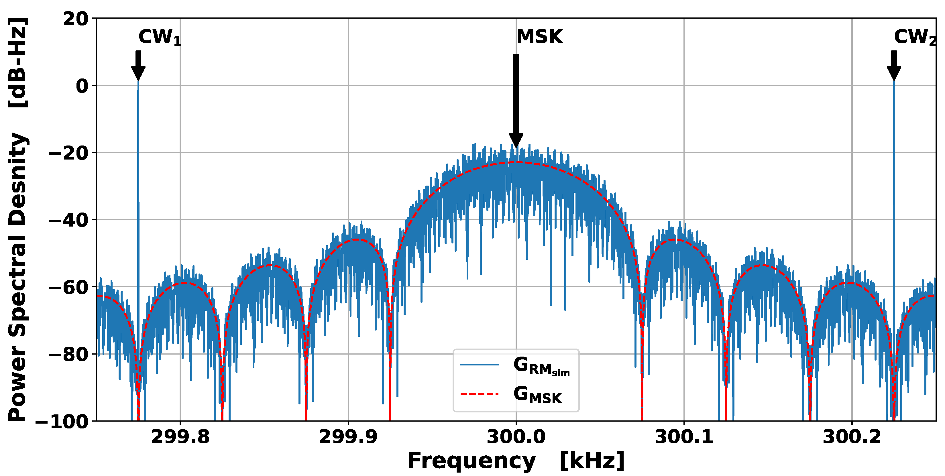
2. The MF R-Mode Signal

The system shares the medium with a frequency division multiple access (FDMA) scheme in which a bandwidth of 500 Hz in the European area is allocated to each transmitter. Different geographical regions might have slightly different allocation strategies that are not considered in this paper. The transmitted MF R-Mode signal is composed of a minimum shift keying (MSK) component, which contains the D(ifferential)GPS information, and two aiding carriers indicated as $C{W}_1$ and $C{W}_2$ placed, respectively, at $f_{MSK}-225$ Hz and $f_{MSK}+225$ Hz, where $f_{MSK}$ is the center frequency of the channel and carrier frequency of the MSK signal. Figure 1 presents the power spectral density (PSD) of a simulated MF R-Mode signal for one channel with a center frequency of 300 kHz (blue line). The different signal components are indicated, and the theoretical PSD of the MSK signal is also presented (red dashed line) to better distinguish them.

The MF R-Mode receiver exploits the aiding carriers to perform ranging by computing their phase. By knowing that at the transmitter side at each full second the phase is zero, the observed phase can be directly translated to a distance measurement. The tracking stage is used to compute the evolution of the phase over time to describe the receiver movement and clock drift. Due to the signals’ wavelength of about 1 km and an approximate service coverage of 300 km, the phase observations are affected by ambiguities. Such ambiguity can be initially solved by performing a calibration procedure by using GNSS for few seconds [4] or by using an apriori knowledge of the location of the receiver. As an alternative, the phase obtained by mixing the of two aiding carriers, referred to as the beat signal phase, can be used to solve the ambiguity since the resulting wavelength is about 666 km. As discussed, the first step of the receiver is the computation of the CW phase. To do that, the discrete Fourier transform (DFT) or its fast implementation, also known as fast Fourier transform (FFT), is used due to the efficiency of the estimation process and low computational complexity. Additionally, the FFT provides the estimates for all the channels in view in one shot. To bound the performance of the phase estimation process, usually the Cramer–Rao Lower Bound (CRLB) is adopted, which describes the optimal achievable performance of an unbiased estimator [9]. Each estimator can be compared with such a bound, and if the estimator attains the bound the estimator is said to be efficient. The CRLB for the phase estimation of the CWs in the MF R-Mode signal is given in [10], where the author describes the assumptions and validity criteria in detail. Under additive white Gaussian noise (AWGN) and by assuming that the bit sequence of the MSK signal is uniformly distributed, the bound for the phase estimate is

$${{\sigma }_{CRLB}}^2\left({\varphi }_{CW}\right)={\displaystyle \frac{2{{\sigma }_n}^2}{A_{CW}^{2}L}}={\displaystyle \frac{{{\sigma }_n}^2}{P_{CW}L}},$$

(1)

where ${{\sigma }_n}^2$ is the noise power, $A_{CW}$ is the amplitude of the sinusoidal tone, and L is the number of samples. The formula can also be expressed by using the sinusoidal tone power since $P_{CW}=\left(A_{CW}^2\right)/2$. By using Equation (1), the optimal achievable performance can be predicted. The challenge now is to properly estimate the noise power and the amplitude of CW to finally obtain the prediction that can be used to monitor the received signal quality under optimal propagation condition.

3. Definition of the Signal Quality Indicator

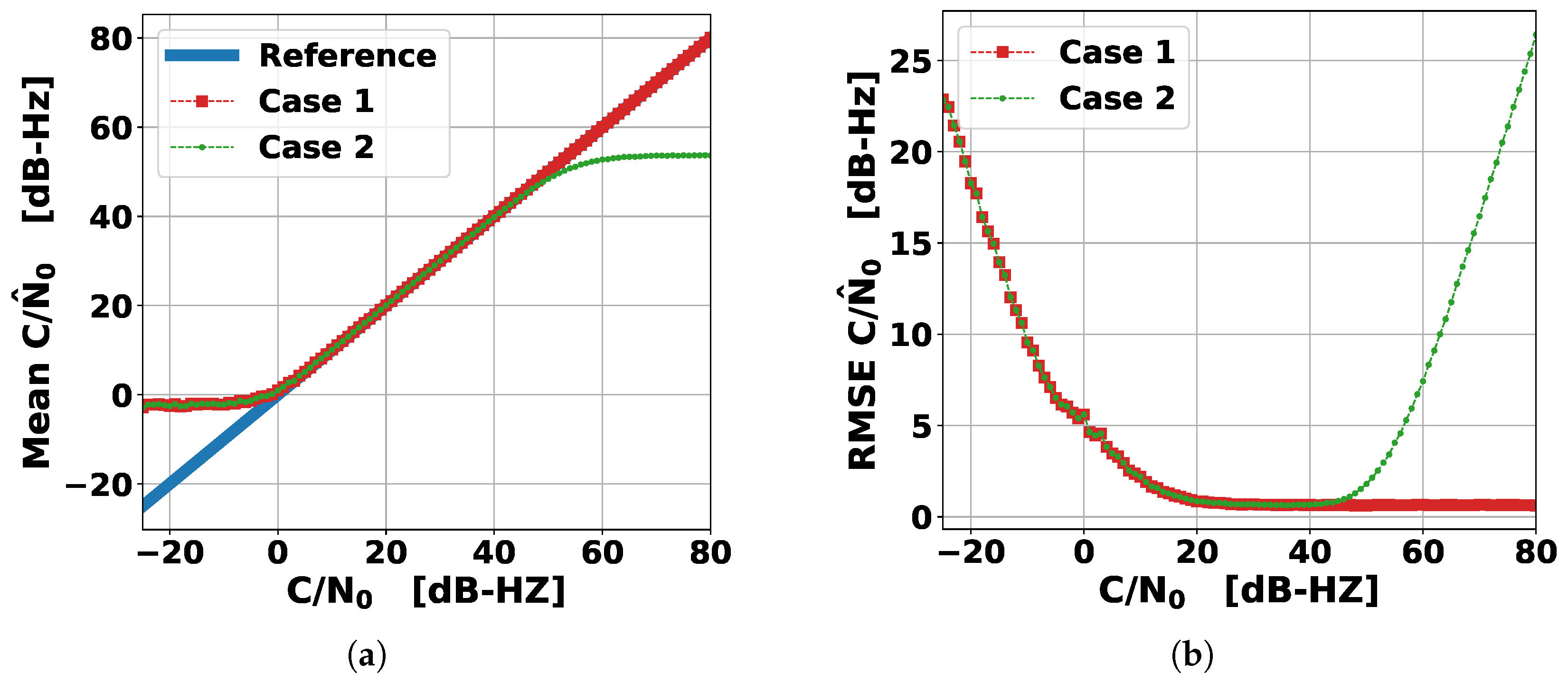
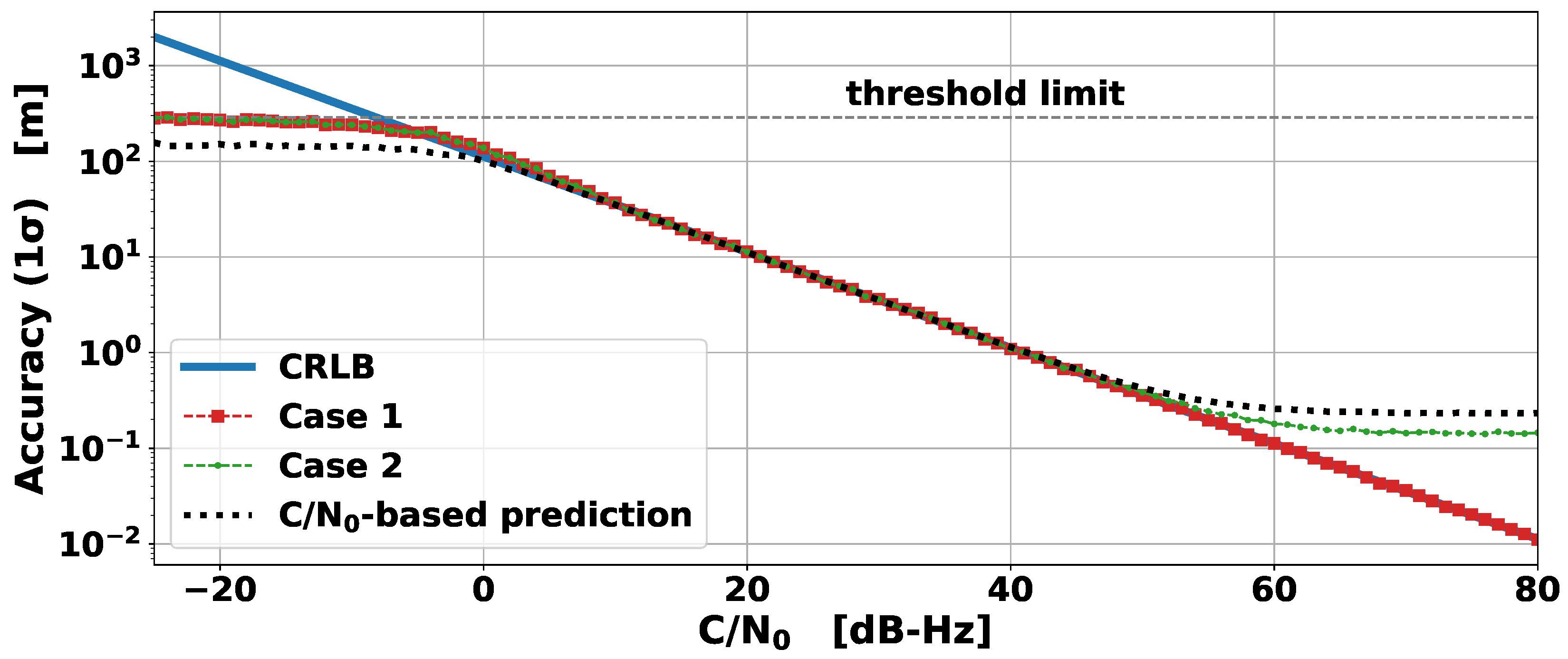
In principle, to define a signal quality indicator we would need to estimate the amplitude or power of the CWs and noise floor level. Such information could be retrieved from the DFT directly, reducing the complexity of the receiver due to the fact that the DFT is already used to perform the phase estimation. Let us assume we have L samples of the real received signal x obtained with sampling frequency $f_s$. The DFT returns L complex numbers $Z_k$

$$Z_k=\sum _{l=0}^{L-1}{x}_n{e}^{-{\displaystyle \frac{j2\pi lk}{L}}}k=0,\dots ,L-1.$$

(2)

It is known that the DFT of a real signal has Hermitian symmetry [11]; hence, only the positive frequency component can be considered, which is for $k=0,...L/2-1$ for even L. The complex number $Z_k$ represents the contribution of the signal with frequency $k{f}_s/L$, and by selecting k such that $\left(k{f}_s\right)/L=f_{CW}$ we can compute amplitude $A_{CW}$ and phase ${\varphi }_{CW}$ of the aiding carrier as

$$A_{CW}={\displaystyle \frac{\left|Z_{CW}\right|}{L}},$$

(3)

$${\varphi }_{CW}=\mathrm{atan}\left\{\mathrm{imag}\left(Z_{CW}\right),\mathrm{real}\left(Z_{CW}\right)\right\}.$$

(4)

From the DFT, one can compute the PSD as follows:

$$\mathbf{P}={\displaystyle \frac{1}{L{f}_S}}\mathbf{ZZ}*,$$

(5)

where $\mathbf{Z}*$ is the complex conjugate of $\mathbf{Z}$. In case of AWGN, the noise power is given by [11]

$$P_n={\sigma }_n^2={\displaystyle \frac{N_0}{2}}{f}_s,$$

(6)

where $N_0/2$ is the noise power density, which can be estimated by using the PSD. Therefore, we can define the carrier to noise density ($C/N_0$)

$$C/N_0={\displaystyle \frac{P_{CW}}{N_0}}={\displaystyle \frac{A_{CW}^2}{2N_0}},$$

(7)

by substituting Equation (7) in (1), the bound can be written as a function of the $C/N_0$ as follows:

$${{\sigma }_{CRLB}}^2\left({\varphi }_{CW}\right)={\displaystyle \frac{2{\sigma }_n^2}{A_{CW}^{2}L}}={\displaystyle \frac{f_s}{2LC/N_0}}.$$

(8)

Therefore, under the optimal propagation condition and with an efficient estimator, the receiver performance can be described by Equation (8).

To estimate the power noise density $N_0$, an average value of the PSD, excluding the sinusoidal tone contribution $P_{k_{CW}}$, can be calculated as follows:

$$N_0=2\overline{P}={\displaystyle \frac{2}{L}}\sum _{k=1}^{{\displaystyle \frac{L}{2}}-1}{P}_k\forall k\ne k_{CW},$$

(9)

where $\overline{P}$ is the mean value of the P. Equation (9) holds only if we have a single continuous wave in AWGN. For the R-Mode signal, this is clearly not the case due to the presence of nearby MSK. Moreover, in real applications the full sampling bandwidth might contain different levels of noise per channel and specific channels might be corrupted by nearby interference that does not affect other channels. However, the FFT can be also seen as a bank of filters applied on the target frequencies $\left(k{f}_s\right)/L$. The bandwidth of each filter depends on $f_s$ and L, and in principle one would need to estimate the noise level within the single filter band. Clearly, this is not possible since the FFT computes the total amount of power entering each filter and cannot distinguish between noise and useful signal component. Therefore, the estimation of the noise floor needs to be carried out locally in the proximity of the target aiding carrier by considering a limited number of samples of $P_k$ around the single tone. Thus, the estimator for the $C/N_0$ becomes

$$C\widehat{/}{N}_0={\displaystyle \frac{P_{k_{CW}}}{\frac{1}{L_B}\left({\sum }_{k=k_{CW}-L_B}^{k_{CW}+L_B}{P}_k\right)}},\forall l\ne k_{CW}$$

(10)

where $L_B$ is the number of points considered on the left and right side of the CW. The accuracy of the estimated $C\widehat{/}{N}_0$ depends on $L_B$, $f_s$, and L used for the DFT; the power allocated for the MSK and CWs; as well as the noise power and nearby interference. The next section presents some results based on simulations.

4. Simulation

To evaluate if Equation (10) can be an appropriate measure of the received signal quality, we perform Monte Carlo simulations. The following signal cases are considered and compared:

• Case 1: Single tone with AWGN
• Case 2: Single channel R-Mode signal (MSK + CWs) in AWGN

It is important to specify that the simulated MSK bit sequence is generated such that bits are random and evenly distributed. This is also quite close to the real MSK bit distribution. For both cases, we assume the reference CW to be located at 300.225 kHz and the channel center frequency to be 300 kHz. Therefore, the spectrum looks like the one represented in Figure 1. We also assume that 50% of the power is allocated to the MSK, whereas 25% is allocated to each CW. We can fix the sampling rate to 1 MS/s, a common value that is used in our receiver, and fix $L_B=25$. If the number of samples for the FFT is $L=1$ MS, the resolution of the FFT is 1 Hz and the bandwidth on which the noise density is calculated is approximately 50 Hz. This means that the noise (and interference of the MSK) is evaluated within the transmitter channel around the target CW. A total number of 1000 runs are simulated for each case and for each value of $C/N_0$. Figure 2 presents the mean value (a) and root mean squared error (RMSE) (b) of the estimate $C\widehat{/}{N}_0$ in dB-Hz for different values of the true $C/N_0$ used in the simulation.

It appears clear that for the case of a single tone in AWGN, the red squared line, the estimated mean value is matching the reference, which is the true value (blue line). For values below 7 dB-Hz, the curve starts to diverge due to the fact that noise power becomes too strong. It can be seen that, by increasing the value of $N_0$, the estimated ($C\widehat{/}{N}_0$) tends to 0 as the amplitude of the CW becomes hidden in the noise.

This behavior is similar for the R-Mode signal case represented by the green line. On the other side, for values of $C/N_0>42$ dB-Hz the estimated mean value is diverging from the reference line and tends to a constant value. This is due to the fact the noise floor is estimated over a 50 Hz bandwidth by using the side bins of the DFT, which are affected by the presence of the MSK side-lobes, similar to a self interference effect. As the noise decreases, the presence of the MSK remains constant, hence the estimated $C\widehat{/}{N}_0$ level will also stay constant and differ from the true value. Regarding the RMSE of the estimate, it can be seen that it increases as the $C/N_0$ level decreases, as expected. Therefore, for $C/N_0<42$ dB-Hz the results for the two cases are similar, whereas for $C/N_0>42$ dB-Hz there is a concrete difference. While the RMSE approaches a constant value for the single tone case, the RMSE increases considerably for the R-Mode case due to the bias of the $C\widehat{/}{N}_0$ estimation.

Figure 3 presents the accuracy of the phase estimation in meters obtained in simulation for the two specific cases. In particular, the RMSE of the phase estimation is given for the single tone case (red) and for the R-Mode signal (green). Additionally, the CRLB for the single tone (blue) and the predicted accuracy (black) obtained by using the estimated values of $C\widehat{/}{N}_0$ for the case 2 are also presented. Good agreement between the curves is visible for $C/N_0$ between 7 and 42 dB-Hz. Below 7 dB-Hz, the signal is strongly compromised by the noise. The estimated RMSE approaches the theoretical limit of $\lambda \sqrt{(1/12)}$ (represented by the horizontal gray dotted line) with the $\lambda$ wavelength of the signal, deriving from the fact that the distribution of the observed phase becomes uniform at $[0,2\pi )$. However, for $C/N_0$ below 7 dB-Hz the signal should not be considered in the positioning algorithm; hence, it is not important to focus on that part of the results, and they are only shown for the sake of completeness.

Above 42 dB-Hz, the CRB and the RMSE for the single tone overlap very well, whereas the result is slightly different when the full R-Mode signal is used. In such a case, we can observe that the RMSE of the phase estimate is a bit better then the predicted curve. Therefore, the predicted curve appears to be like an upper bound of the true RMS phase error. The RMS of the phase error does not follow the CRLB at high $C/N_0$ due to the interference of the MSK. Nevertheless, the accuracy level at this point is in the sub-meter range domain, which is far above the target accuracy of the MF R-Mode system and, in reality, difficult to achieve due to the presence of additional source of error such as the residual error of the atmospheric and ground-wave delay factors (AGDF) [12,13].

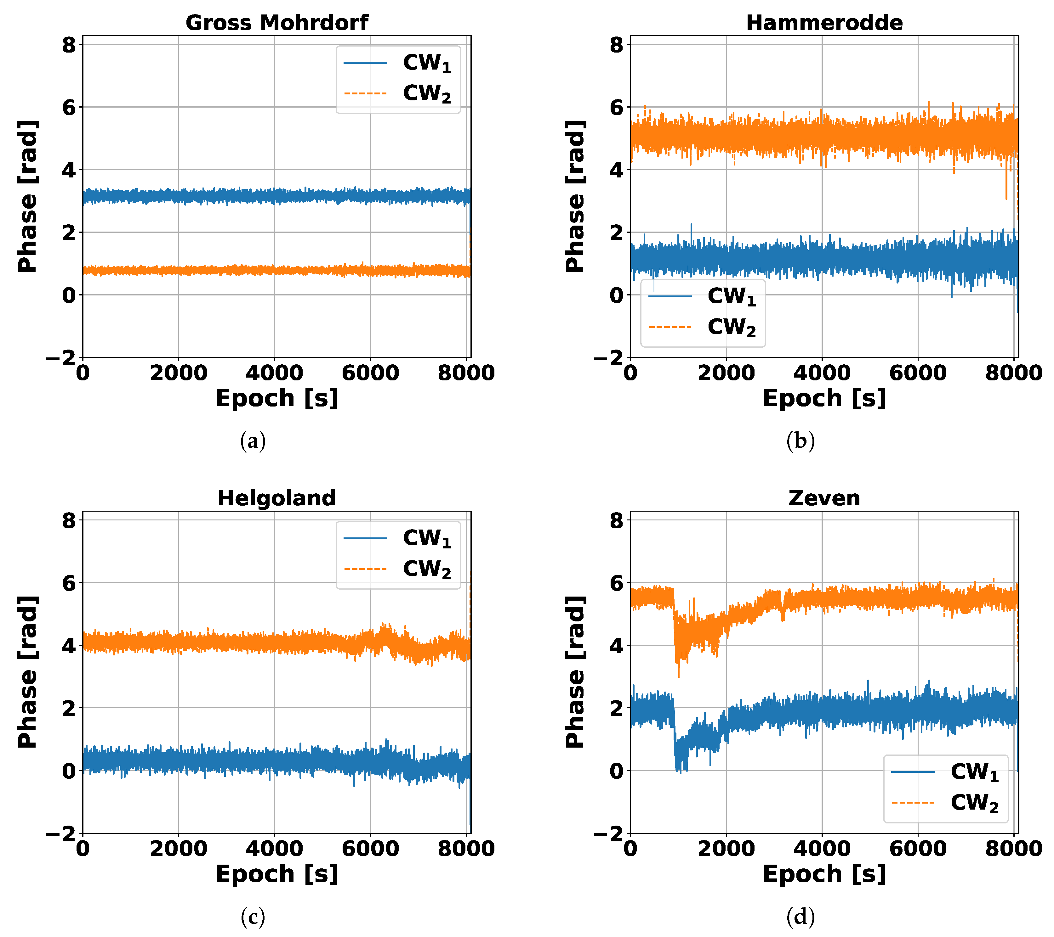
5. Real Data Analysis

Real data are used to validate the usability of the defined $C/N_0$ as a measure of the signal quality under optimal propagation conditions, i.e., without biases. In this paper, we use data from a measurement campaign conducted in September 2023 at a static location on Fehmarn island. The map represented in Figure 4 shows the location of the monitor receiver as an orange triangle, and the MF beacons, which were received as blue circles. As is visible in the map, four stations were received, namely, Groß Mohrdorf, Hammerodde, Zeven, and Helgoland, for a total of eight CW signals.

We are aware that during the measurement, the setup was experiencing some issues that could have caused a noise level increase. Despite the ranging performance loss, this allowed us to evaluate whether the $C/N_0$ parameter could still be used for monitoring purposes under non-nominal noise conditions. The measurements were obtained with a 1 Hz sampling rate.

The standard deviation of the phase error was computed such that a comparison with the predicted accuracy could be carried out. Even if in a static location the phase estimation is in general quite stable, due to the fact that a high accurate rubidium clock is used in the receiver, biases can still be introduced by the station hardware itself. To compensate for these biases, a moving averaging filter is used. Figure 5 presents the phase estimation of both CWs (blue and orange) for the four stations. It appears clear that for some stations, i.e., Helgoalnd and Zeven, time varying biases arise, which must be properly compensated for to achieve optimal positioning performance. In the future, this compensation parameter will be computed by the R-Mode service provider and transmitted to the users with the navigation message. On the contrary, the phase estimation for Groß Mohrdorf and Hammerode was quite good and stable. Once the biases are removed, the standard deviation of the phase can be evaluated and compared with the expected ranging accuracy by using the estimated $C\widehat{/}{N}_0$ in Equation (8).

Figure 6 shows the 2D histogram of the phase standard deviation ($1\sigma$) evaluated over a moving window of 30 samples as a function of the estimated $C/N_0$. To reduce the noise of the $C\widehat{/}{N}_0$ estimation, a moving averaging filter of 30 samples length is applied. Moreover, the ${\widehat{C/N}}_0$ estimate of all the eight CWs is aggregated and used to build the histogram. The data are represented by the gray scale points. Due to the fact that the data were recorded in a static location, the full range of $C/N_0$ values was not observable, which explains the presence of data gaps in the histogram. The predicted accuracy, estimated with Equation (8), is also visible as a red dashed line. As it appears in the figure, the estimated accuracy becomes noisier when the actual $C/N_0$ decreases. This is reasonable as the variance of estimated signal amplitude phase variance increases with the increase in the noise [9]. On the other hand, if the true $C/N_0$ increases or, equivalently, the noise level decreases, its estimate also improves. This agrees with the results obtained in the simulation. In general, it can be observed that the data fit the theoretical curve quite well, which means that the estimated ${\widehat{C/N}}_0$ is a valuable measure of the signal quality under optimal propagation conditions and can be used to predict signal ranging performance. Nevertheless, a small bias between the data and the theoretical lower bound is visible, especially for smaller values of $C/N_0$. To compensate for this bias and to cover the potential residual error due to AGDF mismatch or transmitter instabilities, an inflation factor could be considered to scale up the actual predicted variance of the measurements. In the future, we plan to extend this study by analyzing longer data sets and try to better characterize the different error sources.

6. Conclusions

The paper presents a straightforward approach to define and compute a signal quality indicator, namely, the carrier to noise density ($C/N_0$) ratio, to predict the ranging performance of the MF R-Mode aiding carriers on the receiver side. The indicator is relevant to perform weighting of the measurements on the positioning algorithm as well as to monitor the signals and support the activity of the service operator. Due to the presence of the MSK and the nature of the system, which is based on FDMA, the $C/N_0$ is estimated locally in the vicinity of the aiding carriers by using the output of the FFT to reduce the computational load of the receiver. Thought not claiming to be an exhaustive analysis of all possible approaches to estimate the received signal quality, the usability of the estimated $C/N_0$ as defined in Equation (8) is validated with Monte Carlo simulation as well as with real data. Only the estimation with one set of parameters is presented in this paper, $f_s=1$ MS/s, $N=1$ MS, and $L_B=25$, and in the future other possible values could be explored in order to optimize the estimation, assessing their impact on the $C/N_0$ estimate and ranging performance prediction. Additionally, the work will be extended to consider larger data sets and include a better characterization of the error sources.

References

1. Johnson, G.; Swaszek, P. Feasibility Study of R-Mode Using MF DGPS Transmissions. Available online: https://www.iala.int/content/uploads/2016/08/accseas_r_mode_feasibility_study_mf_dgps_transmissions.pdf (accessed on 8 January 2024).
2. Johnson, G.; Dykstra, K.; Ordell, S.; Swaszek, P. R-Mode positioning system demonstration. In Proceedings of the 33rd International Technical Meeting of the Satellite Division of the Institute of Navigation (ION GNSS+ 2020), Online, 21–25 September 2020. [Google Scholar] [CrossRef]
3. Jeong, S.; Son, P.W. Preliminary Analysis of Skywave Effects on MFDGNSS R-Mode Signals During Daytime and Nighttime. In Proceedings of the IEEE International Conference on Consumer Electronics-Asia (ICCE-Asia), Yeosu, Republic of Korea, 26–28 October 2022. [Google Scholar] [CrossRef]
4. Grundhöfer, L.; Rizzi, F.G.; Gewies, S.; Hoppe, M.; Bäckstedt, J.; Dziewicki, M.; Del Galdo, G. Positioning with medium frequency R-Mode. Navigation 2021, 68, 829–841. [Google Scholar] [CrossRef]
5. Gewies, S.; Dammann, A.; Ziebold, R.; Bäckstedt, J.; Bronk, K.; Wereszko, B.; Rieck, C.; Gustafson, P.; Eliassen, C.G.; Hoppe, M.; et al. R-Mode testbed in the Baltic sea. In Proceedings of the 19th IALA Conference, Incheon, Republic of Korea, 27 May–2 June 2018. [Google Scholar]
6. Rizzi, F.G.; Grundhöfer, L.; Gewies, S.; Ehlers, T. Performance assessment of the medium frequency R-Mode Testbed at Sea near Rostock. Appl. Sci. 2023, 13, 1872. [Google Scholar] [CrossRef]
7. Interreg Baltic See Region. ORMOBASS. Available online: https://interreg-baltic.eu/project/ormobass/ (accessed on 8 January 2024).
8. Falletti, E.; Pini, M.; Lo Presti, L. Low Complexity Carrier-to-Noise Estimators for GNSS Digital Receivers. IEEE Trans. Aerosp. Elecronic Syst. 2011, 47, 420–437. [Google Scholar] [CrossRef]
9. Kay, S.M. Fundamentals of Statistical Signal Processing: Estimation Theory; Prentice-Hall, Inc.: Upper Saddle River, NJ, USA, 1993. [Google Scholar]
10. Grundhöfer, L.; Wirsing, M.; Gewies, S.; Del Galdo, G. Phase Estimation of Single Tones Next to Modulated Signals in the Medium Frequency R-Mode System. IEEE Access 2022, 10, 73309–73316. [Google Scholar] [CrossRef]
11. Proakis, J.G.; Salehi, M. Digital Communications; McGraw-Hill: New York, NY, USA, 2008. [Google Scholar]
12. Hehenkamp, N.; Rizzi, F.G.; Grundhöfer, L.; Gewies, S. Prediction of Ground Wave Propagation Delay for MF R-Mode. Sensors 2024, 24, 282. [Google Scholar] [CrossRef] [PubMed]
13. Rizzi, F.G.; Hehenkamp, N.; Grundhöfer, L.; Gewies, S. Enhancement of MF R-Mode ranging accuracy by exploiting measurement-based error mitigation techniques. WMU J. Marit. Aff. 2023, 22, 299–316. [Google Scholar] [CrossRef]
Figure 1. Simulated MF R-Mode signal PSD (blue curve). The red dashed line represents the theoretical spectrum of a MSK signal.
Engproc 88 00050 g001
Figure 2. Mean value of the estimated C / N 0 for the two cases compared with the reference line (a) and its RMSE (b) in dB-Hz.
Engproc 88 00050 g002
Figure 3. Ranging accuracy for the two described cases compaerd with the CRLB and the C / N 0 -based predicted accuracy.
Engproc 88 00050 g003
Figure 4. Location of the monitor station (orange triangle) and MF R-Mode transmitters (blue circles) processed at the monitor side.
Engproc 88 00050 g004
Figure 5. Fractional part of the phase in rad for Groß Morhdorf (a), Hammerodde (b), Helgoland (c), and Zeven (d).
Engproc 88 00050 g005
Figure 6. 2D histogram of the computed accuracy ( 1 σ ) as function of the estimated C / N 0 . The predicted accuracy is plotted as dashed red line.
Engproc 88 00050 g006
Disclaimer/Publisher’s Note: The statements, opinions and data contained in all publications are solely those of the individual author(s) and contributor(s) and not of MDPI and/or the editor(s). MDPI and/or the editor(s) disclaim responsibility for any injury to people or property resulting from any ideas, methods, instructions or products referred to in the content.