1. Introduction
In recent years, there has been a great increase in the occurrence of Global Navigation Satellite System (GNSS) jamming. In conflict areas, GNSS jamming is widely deployed to hamper the operations of the opposing force. A good overview of where jamming occurs in the world is provided by the website “GPSJam.org”. The idea behind GNSS jamming is simple; by causing interference, the jammer increases the noise received at a receiver until the receiver can no longer track the desired signals. As the received GNSS signals are extremely weak, in the order of −155 dBW, a low-power interference source can impact a large area. A jammer with a power of just 20 mW might cause GNSS disruptions in an area with a radius of more than one kilometer, which is a surface area of more than 3 square kilometers. This makes GNSS jamming relatively easy to perform and cheap, and it can have a large impact, as many systems rely on GNSS not only for positioning but even more often because of the accurate timing it provides. For this reason, GNSS jamming is becoming increasingly popular among the military and other state actors, in addition to criminals and other actors. The reasons for the use of a jammer range from privacy protection for individuals to protection from GNSS-guided (cruise) missiles.
The presence of an interference source, such as a jammer, will impact the carrier-to-noise ratio (
). The carrier-to-noise ratio is the ratio between the power of the carrier of the desired signal
to the power spectral density of the (thermal) noise
. If the
is suppressed enough, the receiver can no longer track the signals and will lose its lock on these signals. Usually, for Binary Phase Shift Keying (BPSK) signals, such as the Global Positioning System (GPS) C/A code or P(Y) code signals, the threshold where the receiver will lose its lock is around 25 dB-Hz [
1]. However, before the lock is lost, the accuracy of the receiver will deteriorate. This is shown in [
2] through a practical experiment and some basic calculations made to predict the impact on GPS C/A. Also, in [
3], the effect on accuracy is shown in an experimental setup where the accuracy of commercial GPS receivers is assessed under different jamming-to-signal ratios. In the current paper, we delve deeper into the theory behind the impact of a jammer on position accuracy. The focus is on the impact of a Gaussian white-noise jammer with different bandwidths on the GPS C/A code and Galileo E1 signals. As both types of signals are sent using different modulation techniques, with GPS C/A being a BPSK signal and Galileo E1 being a Composite Binary Offset Carrier (CBOC) signal, the effects of jamming are expected to be different.
Theory from the literature will be reviewed, after which this theory will be evaluated by comparing the theoretical results with actual measurements using a high-end GNSS signal simulator and a software-defined GNSS receiver [
4].
1.1. Goal of This Paper
The main goal of this paper is to provide insight into the effects of jamming on the accuracy of GNSS receivers. The main message is that the effective range of a jammer is not equal to the range at which the receiver loses its lock; this range is potentially much larger, depending on the required accuracy of the position solution. This paper focuses on the pseudo-range accuracy under additive white Gaussian noise (AWGN) jamming conditions. Biases are not considered. If the accuracy can be predicted well, this prediction can be used to determine the expected effective range of a jammer, in this case, for an AWGN jammer, for applications where accuracy is critical.
1.2. Layout of This Paper
This paper is organized in the following way. First, the theoretical background on which the prediction of the pseudo-range accuracy is based is given. This theoretical background includes the effect of a jammer on the and the tracking error of the DLL. Next, the experimental setup is explained, after which the results are provided. Finally, the paper is drawn to a close in the Conclusions.
2. The Impact of a Jammer on DLL Noise
Pseudo-range errors are a result of the tracking error of the delay lock loop (DLL), so this is our starting point. The tracking error for a non-coherent DLL discriminator is given by the general expression [
5,
6,
7]
where
is the normalized power spectral density of the signal used,
is the correlator spacing,
is the duration of a code chip,
is the coherent integration time,
is the DLL tracking bandwidth, and
is the receiver’s front-end bandwidth. In (1), the noise and interference are assumed to be white Gaussian noise.
In [
1], a simplified version of (1), specifically for BPSK signals, is given:
As we see in these equations, the accuracy is dependent on the , amongst other parameters. The , however, is the only parameter that can be influenced by an interference source, such as a jammer. So, if we can determine the impact of a jammer on the , we will be able to predict the accuracy of the GNSS receiver while under attack from a jammer.
In the literature, the following expression for the impact of interference with a received power
on the effective
can be found [
7]:
where
is the normalized received power of the desired signal within the bandwidth of the front end of the receiver, and
is a jamming resistance quality factor. This jamming resistance quality factor can be calculated as follows:
where
is the normalized power spectral density of the interference; for an AWGN jammer,
where
is the bandwidth of the jammer. Further, the received power,
, of the signal is expressed as
The normalized power spectral densities for BPSK and CBOC are expressed as
and
Finally, the received power of the jammer for the receiver at a distance
can be calculated by using the well-known Friis law, expressed as
where
is the transmitted jammer power;
and
are the antenna gains for the jammer and receiver, respectively; and
is the wavelength.
Upon inspecting (3), it becomes clear that both the duration of a chip,
, and the jamming resistance quality factor,
, influence the impact of a jammer. A smaller
(a larger chiprate) will reduce the impact of a jammer, so the P(Y) code with a chiprate of 10.23 MHz will be less affected by a jammer than a C/A code with a chiprate of 1.023 MHz. This is, of course, exactly as expected. Similarly, a larger
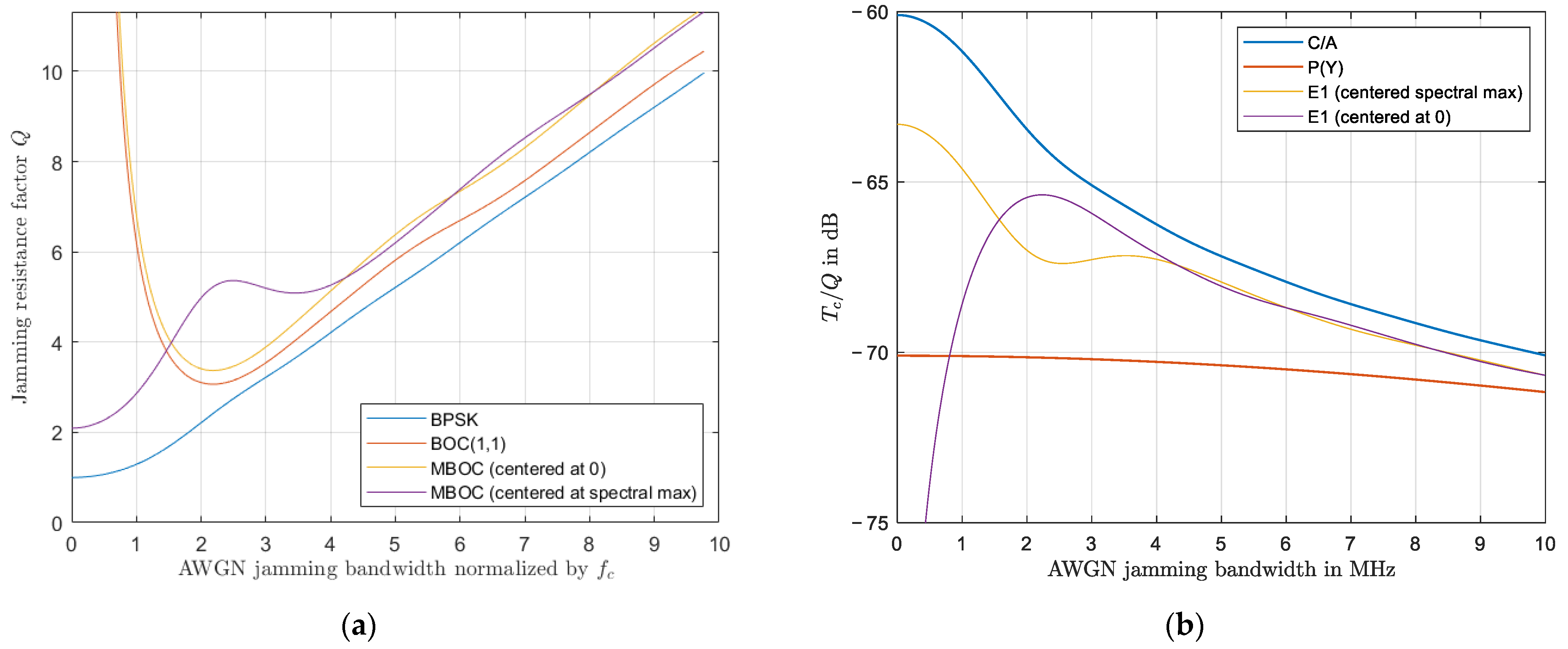
will also reduce the impact of the jammer. In
Figure 1a, the value of
is given for different GNSS signal modulations and a white noise interference source as a function of the normalized (by the chiprate
bandwidth of the interference. From this figure, it is clear that the
for the CBOC modulation is always higher than the
for the BPSK signals. Note, however, that
in this figure is independent of
, so the fact that
is always higher does not indicate that all CBOC GNSS signals are less affected by jamming than BPSK signals, as the
might be different. This is clearly visible in
Figure 1b, where the
, as it appears in (3), is given for the GPS C/A, GPS P(Y), and Galileo E1-OS signals versus the bandwidth of an AWGN jammer. In this figure, a higher
indicates a greater impact of the jammer.
Clearly, the C/A code is most affected by the jammer, while the P(Y) code, although a BPSK signal, performs best because of the 10-times higher chip rate (smaller ).
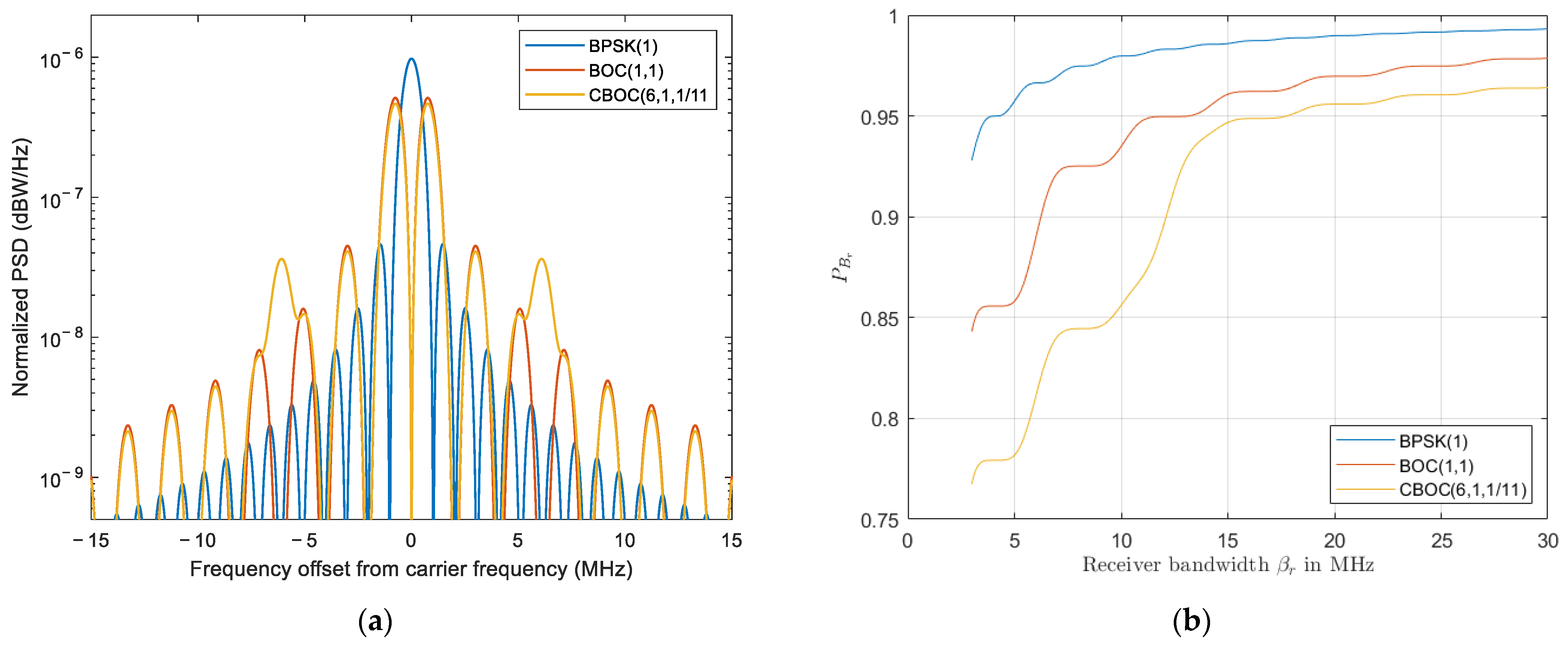
Upon observing
Figure 1a, it also becomes clear that the CBOC modulation performs differently compared to the binary offset carrier (BOC) modulation, despite the fact that the spectra of both signals are quite similar (see
Figure 2a). The difference in performance can be explained by the slight difference in the distribution of the power over the spectrum. The power of the CBOC modulation is spread out over a larger bandwidth, which is visible by the additional power at a frequency offset of around 6 MHz. As long as the power of the received signal within the bandwidth of the jammer is smaller for the CBOC signal, the signal will be less affected by the interference. The difference in bandwidth is also visible in
Figure 2b, where the normalized received power of the signal is given as a function of the receiver’s front end bandwidth. At a bandwidth of 10 MHz, the received power of a CBOC signal is slightly over 85%, while the received power of a BOC(1, 1) signal is around 93%. Even at a bandwidth of over 30 MHz, the difference is still around 1.5%.
Finally, when looking at
Figure 1a, it is notable that the impact of a jammer is maximized by minimizing the bandwidth of the jammer while transmitting at the frequency of the spectral maximum of the target signal. Further, for the (C)BOC signals, the impact of a jammer at the central frequency with a relatively small bandwidth (<0.5 MHz) is, in comparison to the other signals, small. This can be explained by the absence of signal power around the central frequency (see
Figure 1a). If the same jammer is transmitting at the frequency of the spectral maximum, the impact is greater, though not as great as for the BPSK signals. Most jammers, however, do not transmit at a narrow bandwidth, as this may be filtered out by, for example, a notch filter.
Once the impact of the jammer on the is known, the impact on the accuracy of the DLL can be calculated using (1) and/or ().
3. GNSS Jamming Experiment
The equations provided in the previous Section were compared to actual measurements. These measurements were obtained with a software-defined receiver. As over-the-air jamming in the GNSS frequency bands is strictly prohibited, a high-fidelity GNSS receiver was used to generate the satellite signals along with a GNSS jammer signal.
3.1. GNSS Simulator
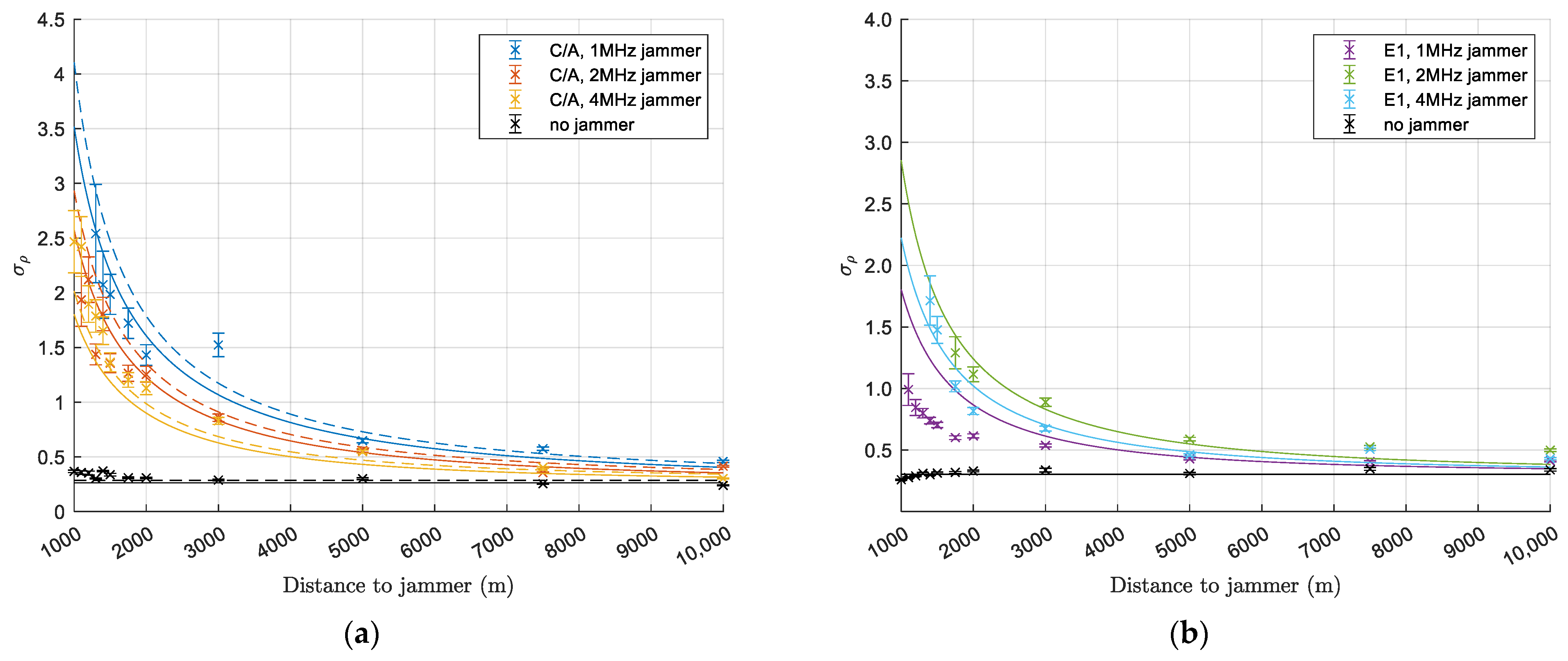
The GNSS simulator used in the experiments was the Orolia Broadsim, which runs the Skydel simulator software. This simulator replicates the GNSS signals, in our case, GPS C/A and Galileo E1, at a chosen position and time. The simulator allows one to place a jammer with user-defined characteristics, like the signal modulation, bandwidth, center frequency, etc., at a certain fixed location or on a moving trajectory. In the experiment, the jammer was set as an AWGN jammer with a transmission power of 20 mW and with different bandwidths of 1, 2, and 4 MHz. The distance from jammer to receiver was varied between 1000 m and 10 km. All simulated experiments were performed 30 m above a flat terrain, with no obstructions of any kind present. The receiver antenna was set to be isotropic in the simulation.
3.2. Software-Defined GNSS Receiver
The receiver used in the experiments was the open-source software-defined GNSS receiver GNSS-SDR [
4]. A software-defined receiver was chosen because it allows one to exactly define the tracking parameters that do influence the accuracy of the receiver. With commercially available receivers, the user usually has no control over these parameters, which complicates the theoretical prediction of their accuracy. The signals were captured using a USRP B210 front end, which was directly connected to the simulator output using a coax cable, so no signals were transmitted over the air. The signals were captured at a sample frequency of 16 MHz as 16-bit IQ data at a central frequency of 1575.42 MHz.
For GPS C/A code tracking, an early-minus-late discriminator was used, with an early-late spacing of 0.4 chips, a DLL loop bandwidth of 0.25 Hz, and an integration time of 10 ms. For Galileo E1 tracking, the GNSS-SDR very-early-minus-very-late discriminator was used, with an early-late spacing of 0.2 chips. The very-early-late spacing was set to be equal to the early–late spacing such that the very-early-minus-very-late discriminator effectively became an early-minus-late discriminator. This setup might result in ambiguity problems due to the additional correlation peaks of the CBOC modulation. This problem, however, was not observed in these experiments. The loop bandwidth for E1 was set to 0.25 Hz, and the integration time was set to 8 ms. The output of the receiver was configured as RINEX files, which contain the pseudo-range, carrier phase, and measurements of the tracked satellites, with a rate of 10 measurements per second.
3.3. Experimental Setup
The experiments were performed in the following way: The first 1.5 min were measured without the jammer being active to allow the receiver to obtain a fix, usually within 25 s, and establish a baseline for performance without jamming. After 1.5 min, the jammer was turned on, and after 3 min, measurement ceased. This process was repeated for distances between the jammer and receiver from 1000 m up to 10 km and for the different jammer bandwidths of 1, 2, and 4 MHz.
The duration of the captured signals was limited by the hardware used to log the USRP-B210 output. Due to the hardware limitations, the maximum file size of the log files was 12 Gb, which led to a maximum duration of only 3 min.

