

A Novel Approach for Classifying Gliomas from Magnetic Resonance Images Using Image Decomposition and Texture Analysis †

 , ,
, ,
Abstract
1. Introduction
2. Related Works
2.1. Research Gaps
2.2. Key Contributions
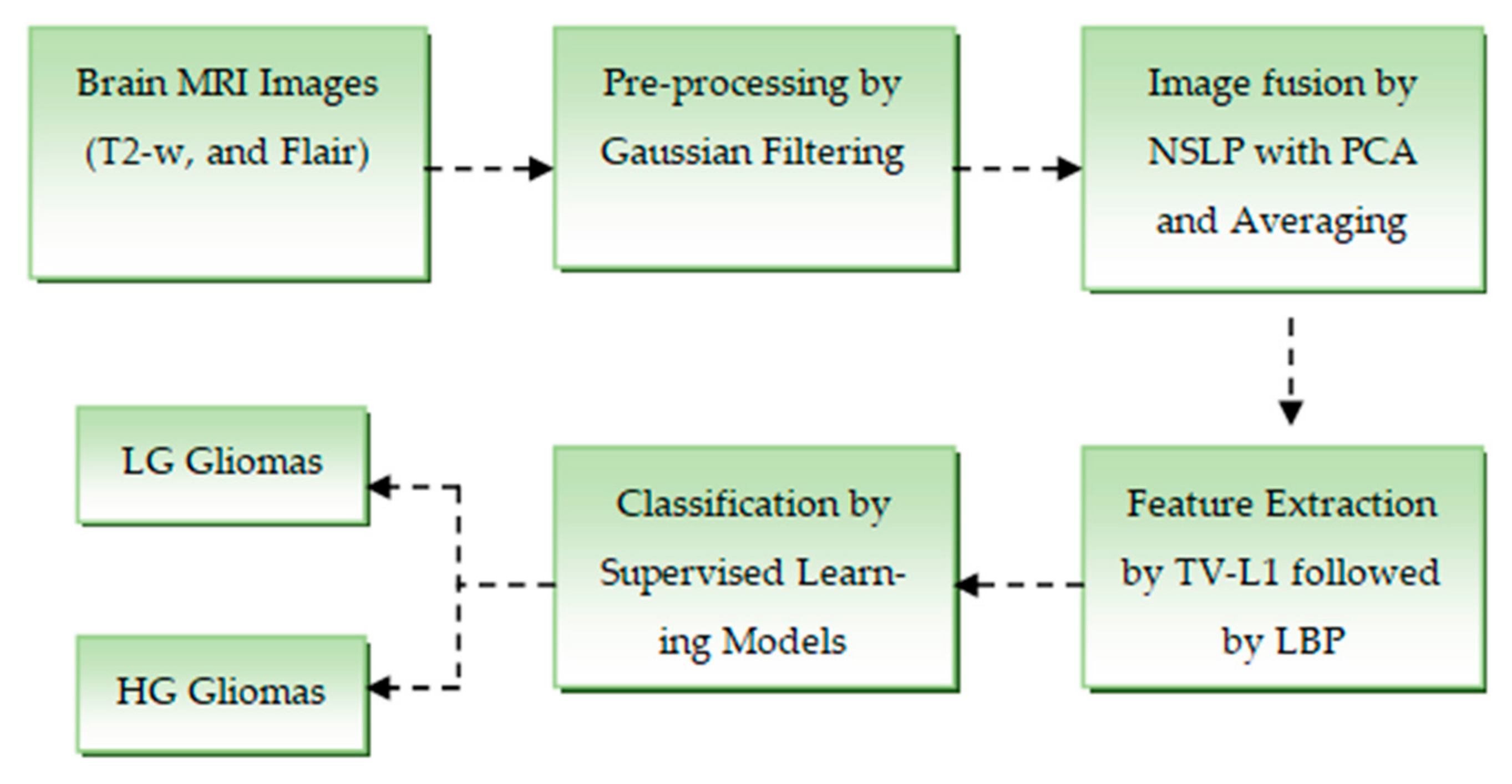
- With the help of GF, we significantly smoothen brain MRI images by eliminating unnecessary details that could affect classification. Further, to improve the visibility of glioma boundaries, we employed NSLP, since it preserves important high-frequency details. This allows us to differentiate LG and HG tumors relatively well;
- TV-L1 separates essential tumor structures (cartoon component) from noise and minor texture variations, aiding in robust feature extraction. Further, we passed LBP through the texture component of TV-L1 decomposition to capture local patterns and edge information that improve the feature representation for machine learning classifiers. Due to this strategic combination, the proposed model attained better performance compared with the existing models
3. Materials and Methods
3.1. Materials
3.2. Pre-Processing
3.3. Brain MRI Image Fusion
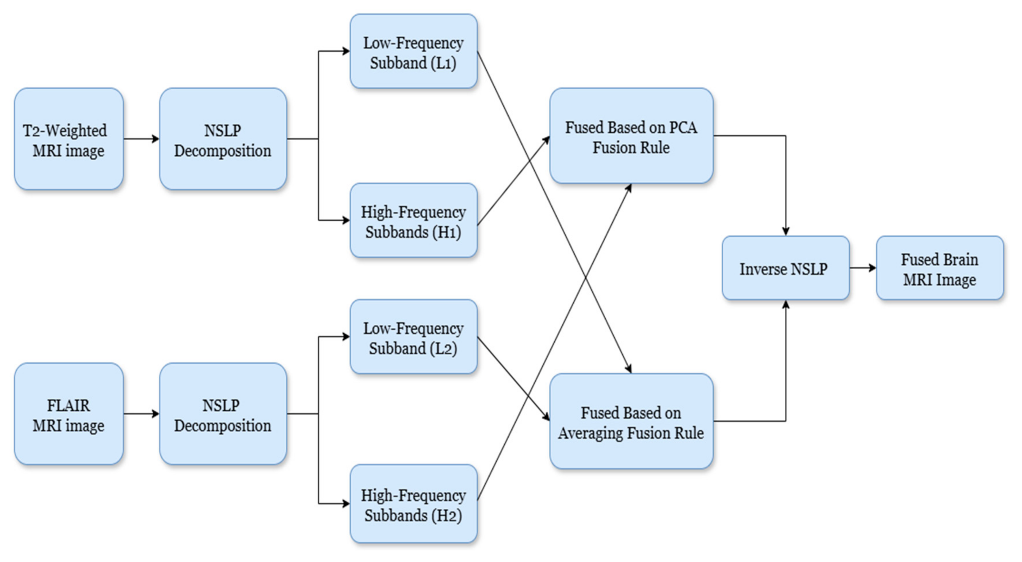
- Image Decomposition: To achieve image decomposition, in this work, we introduced the NSLP-based decomposition approach [16]. NSLP is a multi-resolution analysis strategy that subdivides images into a set of subbands (low-frequency and high-frequency) at different scales and orientations. In this work, we introduced a two-stage NSLP decomposition to decompose the enhanced brain MRI gliomas, resulting in three subbands: one low-frequency (LF) and two high-frequency (HF) subbands. Here, LF subbands illustrate coarse structures, whereas HF subbands illustrate fine details and edges. Further, to improve detection accuracy, these subbands are concatenated using image fusion techniques. To fuse the HF subbands, we utilized principal component analysis (PCA), while for LF subbands, the averaging rule is considered as the fusion rule. Via this process, we can preserve the relevant image details and enhance the overall accuracy of the model;
- High-Frequency Fusion: The HF subbands of both brain MRI glioma images are concatenated using a PCA-based fusion rule, as introduced by Vijayarajan et al. [17]. Here, PCA recognizes the most meaningful principal components within the image. Therefore, by employing PCA on the HF subbands, we can select and combine the components that capture the most significant details from both modalities, resulting in the HF fused subband;
- Low-Frequency Fusion: Here, the LF subbands from both brain tumor images (T1-weighted and FLAIR) are merged using a simple approach, namely averaging [17]. The pixel values of corresponding LF subbands of both images are averaged to attain the fused LF subband;
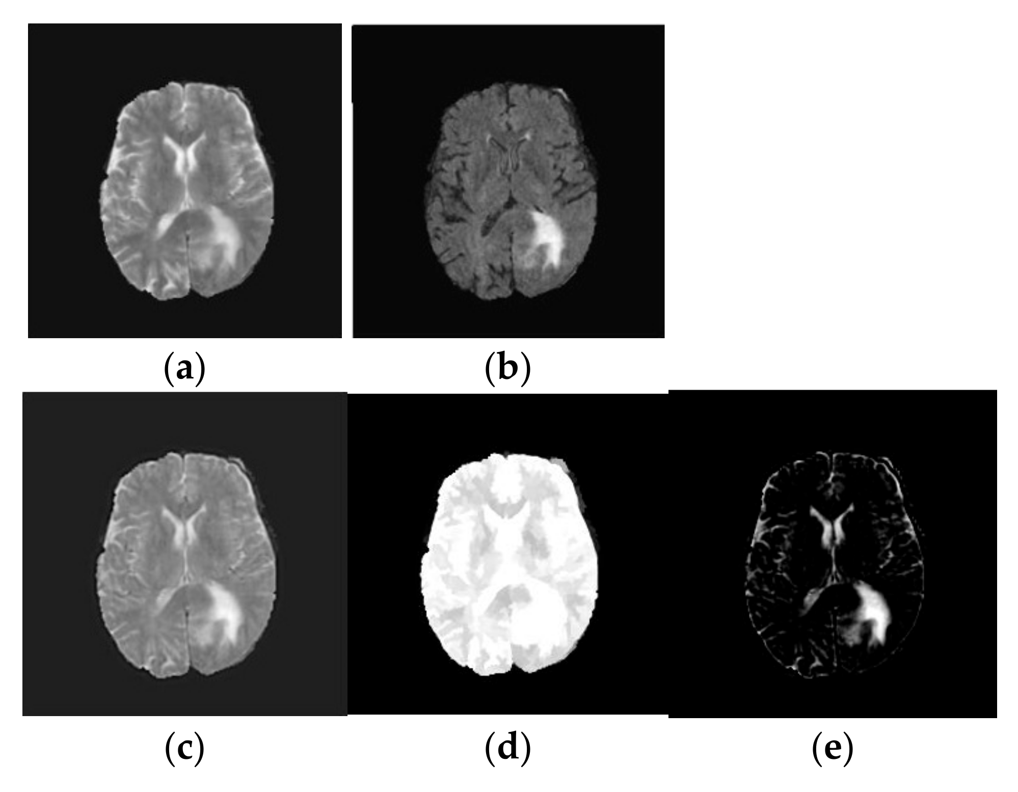
- Image Reconstruction: Finally, the fused low-frequency and high-frequency subbands are recombined using the inverse NSLP. This process reconstructs the final fused MRI image, which is expected to contain the complementary information from both T1-weighted and FLAIR images. The implications of the fused process are shown in Figure 3.
3.4. Feature Extraction
- TV-L1 Decomposition: The primary objective of our method is to decompose the fused image, into two distinct components: a piecewise smooth (geometric) component and a texture component. The geometric component represents the smooth regions and boundaries of the image, while the texture component captures oscillating features, including edges and noise. In medical imaging, the texture component often contains critical structural details that are essential for tasks such as tumor classification. These structural details can be effectively extracted using the TV-L1-based cartoon-texture decomposition technique. The TV-L1 method separates the fused brain MRI tumor image into two components: the cartoon (geometric) component and the texture component, as outlined in [18]:where gives the cartoon part and which characterizes the geometric component of the fused image. Similarly, represents the texture part of the fused image. The cartoon component of the fused image is attained by minimizing the following objective function [18]:where represents the gradient operator and λ defines the regularization criteria which is a trade-off between the fidelity criteria and regularization term. In this work, we chose λ as 0.1. Similarly, denotes the image domain and the symbol represents L1 normalization. The first part of Equation (2) represents the TV of cartoon component and the second part specifies the fidelity to make the cartoon part keep close to the fused image, and they are calculated over the image domain Ω. The solution to Equation (2) is resolved by the following optimization [19]:where and represent the forward and backward differences. provides the magnitude of gradient. The parameter l provides the iteration index. In this, we chose l as 50. is defined as changes in time, and and indicate discrete spatial distances of the image grid. φ and ε (0.00001) are constants. The resultant outcome of TV-L1 decomposition is shown in Figure 3.
- Local binary patterns (LBPs): To further enhance classification performance, local features were extracted from the texture component of the fused image () using the LBP technique [20]. LBP is a simple yet powerful texture descriptor that labels the pixels of an image by thresholding the neighborhood of each pixel and converting the result into a binary number. It captures local texture patterns by comparing the intensity of each pixel with its surrounding neighbors, creating a binary code that represents the texture. The key advantage of LBP lies in its ability to capture distinct local texture patterns while establishing spatial relationships between them. Additionally, its robustness to variations in illumination and high computational efficiency make it an excellent choice for tasks such as brain tumor classification. In this work, we consider radius (R) as one, the number of neighboring pixels for thresholding as eight, and a variant of uniform LBP.
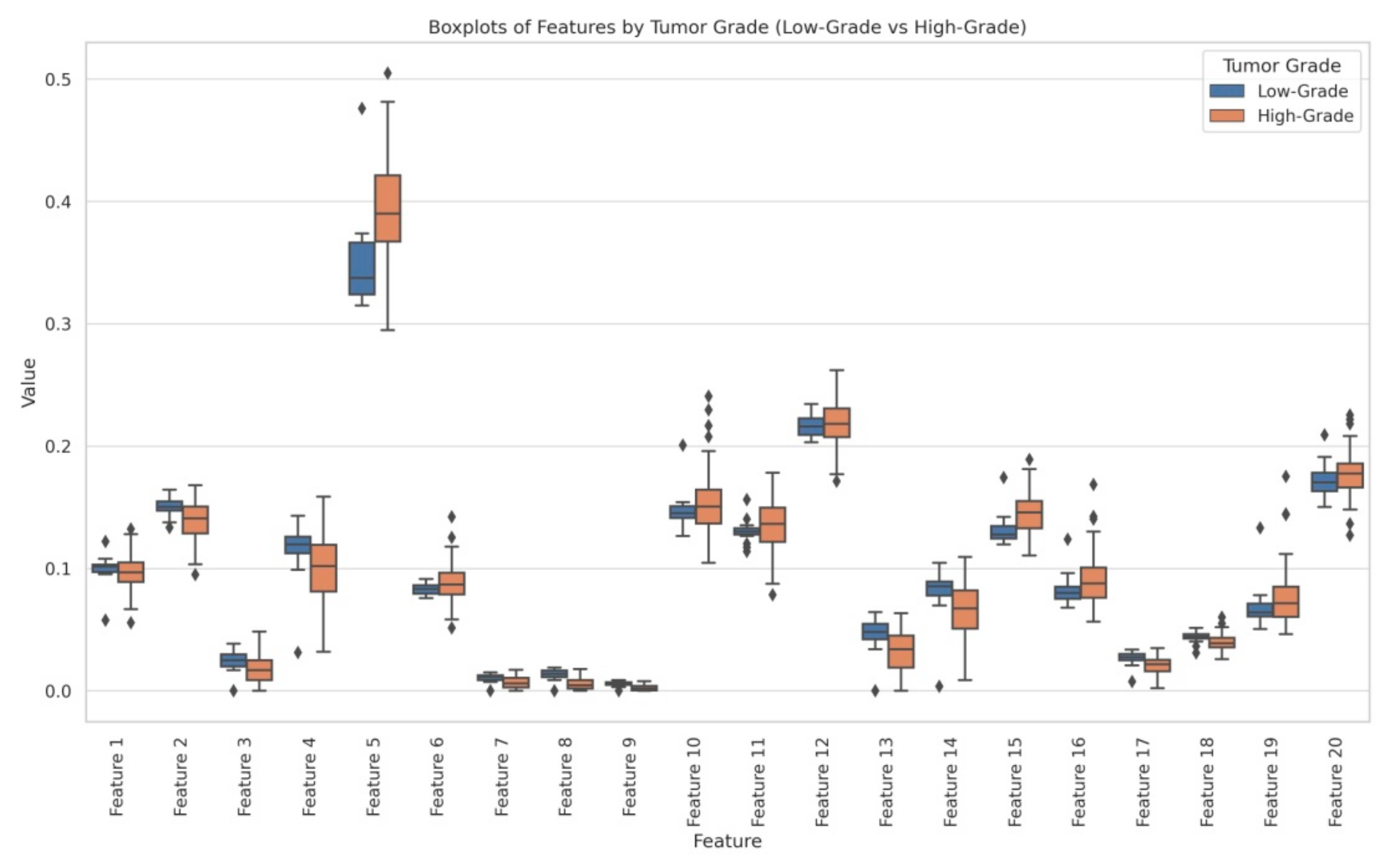
- Statistical analysis: By the above-mentioned feature engineering process, we obtained 20 radiomic features and they were analyzed through independent t-tests and ANOVA to identify significant differences between LG and HG. The statistical analysis revealed that several features exhibited significant differences between LG and HG:
- Feature 2 (t-test p = 0.000052, ANOVA p = 0.0044);
- Feature 5 (t-test p = 0.000742, ANOVA p = 0.00026);
- Feature 7 (t-test p = 0.001887, ANOVA p = 0.00387);
- Feature 8 (t-test p = 0.000005, ANOVA p = 3.73 × 10⁻⁹);
- Feature 9 (t-test p = 0.000006, ANOVA p = 3.04 × 10⁻⁹).
3.5. Classification
4. Results and Discussion
Comparison with the Existing Approaches
- By integrating the modalities of brain MRI tumor images based on the NSLP followed by the fusion strategies, the presented model significantly detects abnormal regions within the brain tumors. Unlike relying on individual imaging sequences, the fusion process enhances tissue information, enabling a more accurate detection of tumor regions. This fusion-based enhancement is a significant advantage of the proposed technique;
- Furthermore, the proposed brain tumor classification methodology outperforms existing techniques by accurately distinguishing LG and HG gliomas from MRI images. This is achieved through an efficient extraction strategy that is TV-L1 decomposition followed by LBP. Here, the TV-L1 identifies crucial details, like patterns and structural features of the images, whereas the LBP provides the edge and corner features. Together, these approaches represent a major contribution of the proposed method, enabling precise and reliable tumor classification.
5. Conclusions and Future Scope
Author Contributions
Funding
Institutional Review Board Statement
Informed Consent Statement
Data Availability Statement
Conflicts of Interest
References
- Ostrom, Q.T.; Price, M.; Neff, C.; Cioffi, G.; A Waite, K.; Kruchko, C.; Barnholtz-Sloan, J.S. CBTRUS statistical report: Primary brain and other central nervous system tumors diagnosed in the United States in 2015–2019. Neuro-Oncology 2022, 24 (Suppl. S5), v1–v95. [Google Scholar] [CrossRef]
- Schneider, T.; Mawrin, C.; Scherlach, C.; Skalej, M.; Firsching, R. Gliomas in adults. Dtsch. Ärzteblatt. Int. 2010, 107, 799. [Google Scholar] [CrossRef] [PubMed]
- Ichimura, K. Molecular pathogenesis of IDH mutations in gliomas. Brain Tumor Pathol. 2012, 29, 131–139. [Google Scholar] [CrossRef] [PubMed]
- Zeng, T.; Cui, D.; Gao, L. Glioma: An overview of current classifications, characteristics, molecular biology and target therapies. Front. Biosci. (Landmark Ed.) 2015, 20, 1104–1115. [Google Scholar]
- Louis, D.N.; Ohgaki, H.; Wiestler, O.D.; Cavenee, W.K.; Burger, P.C.; Jouvet, A.; Scheithauer, B.W.; Kleihues, P. The 2007 WHO classification of tumours of the central nervous system. Acta Neuropathol. 2007, 114, 97–109. [Google Scholar] [CrossRef]
- Sharif, M.; Amin, J.; Raza, M.; Anjum, M.A.; Afzal, H.; Shad, S.A. Brain tumor detection based on extreme learning. Neural Comput. Appl. 2020, 32, 15975–15987. [Google Scholar] [CrossRef]
- Amin, J.; Sharif, M.; Gul, N.; Yasmin, M.; Shad, S.A. Brain tumor classification based on DWT fusion of MRI sequences using convolutional neural network. Pattern Recognit. Lett. 2020, 129, 115–122. [Google Scholar] [CrossRef]
- Chandra, S.K.; Bajpai, M.K. Fractional mesh-free linear diffusion method for image enhancement and segmentation for automatic tumor classification. Biomed. Signal Process. Control 2020, 58, 101841. [Google Scholar] [CrossRef]
- Reddy, K.R.; Dhuli, R. Segmentation and classification of brain tumors from MRI images based on adaptive mechanisms and ELDP feature descriptor. Biomed. Signal Process. Control 2022, 76, 103704. [Google Scholar]
- Hafeez, H.A.; Elmagzoub, M.A.; Abdullah, N.A.B.; Al Reshan, M.S.; Gilanie, G.; Alyami, S.; Hassan, M.U.; Shaikh, A. ACNN-model to classify low-grade and high-grade glioma from MRI images. IEEE Access 2023, 11, 46283–46296. [Google Scholar] [CrossRef]
- Sachdeva, J.; Sharma, D.; Ahuja, C.K.; Singh, A. Efficient-Residual Net—A Hybrid Neural Network for Automated Brain Tumor Detection. Int. J. Imaging Syst. Technol. 2024, 34, e23170. [Google Scholar] [CrossRef]
- Rachmawanto, E.H.; Sari, C.A.; Isinkaye, F.O. A good result of brain tumor classification based on simple convolutional neural network architecture. Telkomnika (Telecommun. Comput. Electron. Control) 2024, 22, 711–719. [Google Scholar] [CrossRef]
- Menze, B.H.; Jakab, A.; Bauer, S.; Kalpathy-Cramer, J.; Farahani, K.; Kirby, J.; Burren, Y.; Porz, N.; Slotboom, J.; Wiest, R.; et al. The multimodal brain tumor image segmentation benchmark(BRATS). IEEE Trans. Med. Imaging 2014, 34, 1993–2024. [Google Scholar] [CrossRef]
- Gupta, K.; Gupta, S.K. Image Denoising techniques—A review paper. IJITEE 2013, 2, 6–9. [Google Scholar]
- Gonzalez, R.C. Digital Image Processing; Pearson Education India: Chennai, India, 2009. [Google Scholar]
- Da Cunha, A.; Zhou, J.; Do, M. The nonsubsampled contourlet transform: Theory, design, and applications. IEEE Trans. Image Process. 2006, 15, 3089–3101. [Google Scholar] [CrossRef]
- Vijayarajan, R.; Muttan, S. Discrete wavelet transform based principal component averaging fusion for medical images. AEU-Int. J. Electron. Commun. 2015, 69, 896–902. [Google Scholar] [CrossRef]
- Le Guen, V. Cartoon + texture image decomposition by the TV-L1 model. Image Process. Line 2014, 4, 204–219. [Google Scholar] [CrossRef]
- Ghita, O.; Ilea, D.E.; Whelan, P.F. Texture Enhanced Histogram Equalization Using TV-L1 Image Decomposition. IEEE Trans. Image Process. 2013, 22, 3133–3144. [Google Scholar] [CrossRef]
- Ojala, T.; Pietikäinen, M.; Harwood, D. A comparative study of texture measures with classification based on featured distributions. Pattern Recognit. 1996, 29, 51–59. [Google Scholar] [CrossRef]
- Vapnik, V. The Nature of Statistical Learning Theory; Springer Science & Business Media: Berlin, Germany, 2013. [Google Scholar]
- Cunningham, P.; Delany, S.J. K-nearest neighbour classifiers—Atutorial. ACM Comput. Surv. (CSUR) 2021, 54, 128. [Google Scholar]
- Loh, W.-Y. Classification and regression trees. Wiley Interdiscip. Rev. Data Min. Knowl. Discov. 2011, 1, 14–23. [Google Scholar] [CrossRef]
- Schapire, R.E. Explaining adaboost. In Empirical Inference: Festschrift in Honor of Vladimir N. Vapnik; Springer: Berlin/Heidelberg, Germany, 2013; pp. 37–52. [Google Scholar]
- Friedman, J.; Hastie, T.; Tibshirani, R. Additive logistic regression: A statistical view of boosting (With discussion and a rejoinder by the authors). Ann. Stat. 2000, 28, 337–407. [Google Scholar]

| Classifier | Key Hyperparameters |
|---|---|
| SVM | Kernel Function: ‘rbf’, and Kernel Scale: ‘auto’ |
| KNN | Num Neighbors: 5, and Distance: ‘euclidean’ |
| DT | Max Num Splits: 10, Split Criterion: ‘gdi’, and Prune: ‘on’ |
| AdaBoost | Num Learning Cycles: 100, and Learn Rate: 0.1 |
| LogitBoost | Num Learning Cycles: 100, Learn Rate: 0.1, and Max Num Splits: 10 |
| Classifier | Performance Metrics (%) | |||||
|---|---|---|---|---|---|---|
| Sensitivity | Specificity | Precision | F1-Score | AUC | Accuracy | |
| SVM | 45.71 | 99.28 | 94.12 | 61.53 | 72.5 | 88.57 |
| KNN | 68.57 | 94.28 | 75 | 71.64 | 81.43 | 89.14 |
| DT | 31.42 | 91.43 | 47.82 | 37.92 | 61.43 | 79.43 |
| AdaBoost | 85.71 | 99.28 | 96.77 | 90.9 | 92.5 | 96.57 |
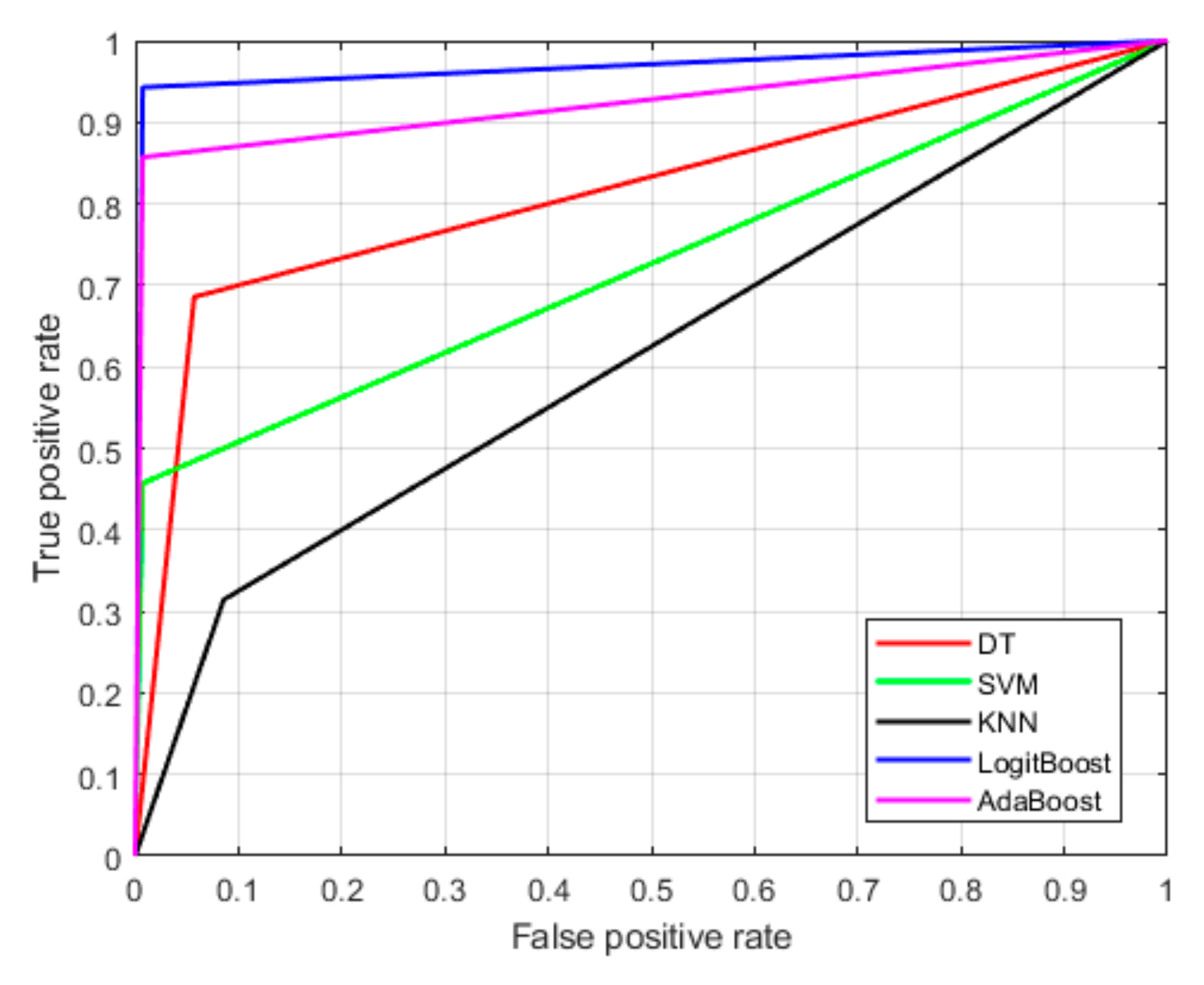
| LogitBoost | 94.28 | 99.29 | 97.05 | 95.64 | 96.8 | 98.29 |
| Method | Evaluation Criteria | Performance Measures | ||
|---|---|---|---|---|
| Sensitivity | Specificity | Accuracy | ||
| ELM [6] | 80% training and 20% testing | 95 | 93 | 96.5 |
| DWT-CNN [7] | 80% training and 20% testing | 98 | 92 | 96 |
| FMFPDE-SVM [8] | 5- fold cross validation | 97.5 | 96.08 | 97.5 |
| ELDP-SVM [9] | 10-fold cross validation | 89.19 | 97.08 | 94.44 |
| CNN [10] | - | 99.88 | 98.88 | 97.85 |
| Hybrid Model [11] | 80% training and 20% testing | 98 | - | 97.59 |
| Customized CNN [12] | 80% training and 20% testing | 95.84 | 90.08 | 94.14 |
| The Proposed | 94.28 | 99.29 | 98.25 | |
Disclaimer/Publisher’s Note: The statements, opinions and data contained in all publications are solely those of the individual author(s) and contributor(s) and not of MDPI and/or the editor(s). MDPI and/or the editor(s) disclaim responsibility for any injury to people or property resulting from any ideas, methods, instructions or products referred to in the content. |
© 2025 by the authors. Licensee MDPI, Basel, Switzerland. This article is an open access article distributed under the terms and conditions of the Creative Commons Attribution (CC BY) license (https://creativecommons.org/licenses/by/4.0/).
Share and Cite
Babu, K.S.; Munigeti, B.J.; Naidana, K.S.; Bapatla, S. A Novel Approach for Classifying Gliomas from Magnetic Resonance Images Using Image Decomposition and Texture Analysis. Eng. Proc. 2025, 87, 70. https://doi.org/10.3390/engproc2025087070
Babu KS, Munigeti BJ, Naidana KS, Bapatla S. A Novel Approach for Classifying Gliomas from Magnetic Resonance Images Using Image Decomposition and Texture Analysis. Engineering Proceedings. 2025; 87(1):70. https://doi.org/10.3390/engproc2025087070
Chicago/Turabian StyleBabu, Kunda Suresh, Benjmin Jashva Munigeti, Krishna Santosh Naidana, and Sesikala Bapatla. 2025. "A Novel Approach for Classifying Gliomas from Magnetic Resonance Images Using Image Decomposition and Texture Analysis" Engineering Proceedings 87, no. 1: 70. https://doi.org/10.3390/engproc2025087070
APA StyleBabu, K. S., Munigeti, B. J., Naidana, K. S., & Bapatla, S. (2025). A Novel Approach for Classifying Gliomas from Magnetic Resonance Images Using Image Decomposition and Texture Analysis. Engineering Proceedings, 87(1), 70. https://doi.org/10.3390/engproc2025087070