1. Introduction
The oil industry is crucial for meeting global energy demands, providing petroleum products through a pipeline network [
1]. To have safe and efficient operation, it is essential to ensure the pipelines are maintained. The main maintenance method used in pipelines is called pigging. The process involved the use of specialized devices known as (pipeline inspection gauges) pigs are inserted through the pipelines for cleaning and inspection. This routine maintenance is crucial for the efficient and safe transport of these resources [
2]. Regular operations are performed on pipelines to address anomalies and ensure smooth oil flow. During this operation, debris or buildup within the pipeline is cleaned to prevent corrosion, improve oil flow, and maintain the pipeline’s integrity [
3]. Although pigging is crucial for maintaining pipeline integrity, our traditional approach to scheduling these tasks primarily depends on manual design specifications, which frequently leads to issues, resulting in time and cost consumption and placing significant pressure on the industry. This current method often disrupts daily operations, leads to overcleaned pipelines, and increases costs. Its ability to predict issues like blockages and buildup before they occur is crucial, even though it does not adapt to real-time conditions [
4]. These restrictions significantly impact the environment and the economy. They also jeopardize our pipelines and consume excessive resources. People are starting to recognize these problems more clearly, and we understand that a data-driven solution is necessary. That is why we plan to utilize machine learning to determine the optimal times for cleaning our oil pipelines.
Machine learning is a skilled detective that analyzes complex datasets, discovers hidden patterns, and finally makes confident predictions [
5,
6]. Machine learning has the capability to transform many industries, like the oil and gas sector. By using real-time and historical pipeline data, machine learning can accurately identify the optimal schedule and locations to carry out pigging operations in oil pipelines [
3]. Moving from a reactive, manual scheduling method to a proactive, data-driven approach can reduce costs and downtime and enhance the integrity of pipelines [
7]. This study seeks to exploit this capability by creating a machine learning-based predictive model to enhance the efficiency and maintenance schedules in oil pipelines. The main objective is to help the oil industry improve efficiency and sustainability while making significant progress in pipeline management and maintenance. Machine learning and predictive modeling have undergone significant progress, leading to transformations in the oil and gas sector. For instance, it is like how individuals learn from experience and predict outcomes based on familiar patterns; these technologies enable oil and gas companies to analyze large datasets, predict potential challenges, make well-informed decisions, and enhance safety and efficiency. Even though there is progress in machine learning utilization in the oil and gas industries, there is still a gap in predicting maintenance schedules for oil pipelines. Previous studies have mostly concentrated on overall pipeline maintenance, but little attention has been paid to planning the best time to schedule pigging. The models we have now mostly predict things like how much wax builds up, and they often look at small pieces of the pipeline [
8]. They miss out on all the tricky details involved in planning the most effective pigging operations.
1.1. Challenges of Pigging Operational in Pipeline Maintenance
Pigging is an important activity in crude oil pipelines, but it has several challenges during operation that impact the integrity and maintenance schedules of pipelines. The main challenge is wax deposition, which occurs when crude oil cools and leads to paraffinic wax accumulation inside the pipeline walls. Excessive wax buildup can increase a drop in pressure, affect flow, and lead to frequent pigging to prevent blockages. If not managed properly, the accumulation of wax can lead to a reduction in operational efficiency and unexpected shutdowns. Variation in flow rate is another significant factor that affects the effectiveness of pigging activities. An optimal flow rate is required for pigs to travel smoothly through the pipeline. Pigs stall is caused by a low flow rate, while excessive wear is caused by a high flow rate. Also, fluctuations in flow rates can lead to uneven accumulation of deposits, which makes it difficult to forecast when maintenance is needed. Pipeline geometry also plays a vital role in the efficiency of pigging operations. Variables such as diameter variations, bends, and branch connections can cause obstacles to the movement of pigs, which leads to a reduction in their ability to remove deposits effectively.
These challenges in pigging operations highlight the need for data-driven predictive maintenance techniques that can optimize pigging schedules based on real-time pipeline conditions. Traditional static maintenance strategies, which normally rely on fixed time intervals, may not solve these dynamic challenges. Therefore, by integrating machine learning models that analyze variation in flow rate, pipeline operators can develop a maintenance schedule that improves the integrity of the pipeline, enhances cost efficiency, and reduces disruption during operation.
There is a gap in the research when it comes to having detailed plans for dealing with this problem. Refs. [
9,
10,
11,
12,
13] concentrate on predicting wax accumulation in pipelines, but there is not much emphasis on how to make sure the cleaning process goes smoothly. This study introduces an approach using machine learning. Therefore, it aims to bridge this gap by developing a predictive model using machine learning that is tailor-made to optimize maintenance schedules in oil pipelines such as pigging operations. It takes data on how fast the oil flow rate moves at different spots along the pipeline to paint a clear picture of how clean the pipeline is. This way, it can determine the best time to start a cleaning operation.
1.2. Limitations of Traditional Pipeline Maintenance Approaches
Condition-Based Maintenance (CBM), Time-Based Maintenance (TBM), and Reliability-Centered Maintenance (RCM2) are three traditional ways of maintaining crude oil pipelines. Each of these techniques has specific features and limits that affect maintenance efficiency and cost-effectiveness [
14,
15].
Condition-Based Maintenance (CBM) improves efficiency by integrating sensors and routine checks to evaluate pipeline conditions instantly. CBM also depends on predetermined thresholds and human perception, notwithstanding its benefits. Because human judgment and threshold settings may not always adequately capture complicated deterioration patterns, this dependency may not always result in the best maintenance practices.
Time-Based Maintenance (TBM) adheres to a set maintenance plan regardless of the pipeline’s actual status. Even though this method provides routine inspections and interventions, it frequently leads to raising operating expenses, needless maintenance tasks, and resource usage without necessarily enhancing pipeline dependability.
Reliability Centered Maintenance (RCM2) is a more sophisticated method that incorporates prioritization strategies and risk-based evaluations. Concentrating maintenance efforts on important pipeline components enables strategic decision-making. However, RCM2 is less flexible to operating conditions dynamically, especially in intricate pipeline networks with fluctuating flow rates and environmental influences, because it necessitates a great deal of expert input and detailed failure mode analysis.
Therefore, considering these drawbacks, machine learning-based predictive maintenance presents a viable substitute by using real-time monitoring and historical data to dynamically improve maintenance plans.
2. Research Methodology
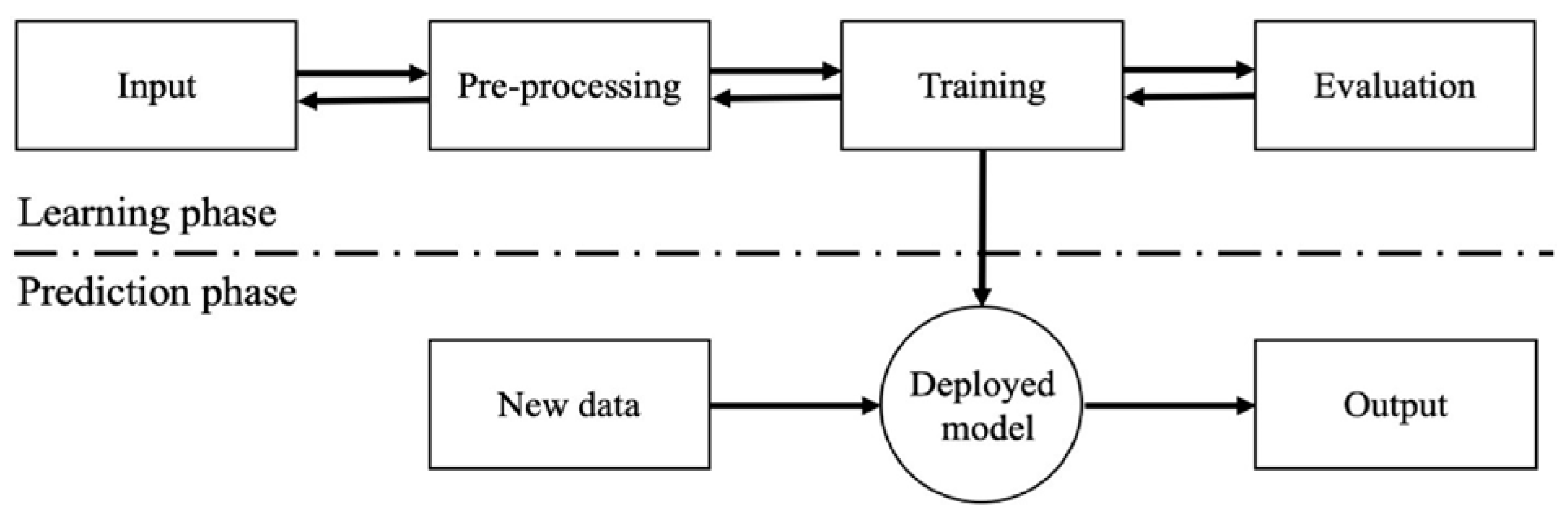
This research introduced a machine learning algorithm to predict maintenance schedules for oil pipelines. It described the key stages taken to develop and deploy machine learning models. Machine learning utilizes algorithms to detect patterns within data, which are subsequently utilized for predictive models’ development [
6]. Historical data on diverse characteristics and properties of pipelines are used to build models for oil pipelines. These data encompass information like the pipeline’s diameter, wall thickness, length, materials, location, type, age, topology, coating type, debris weight, frictional force, pig speed, oil speed, discharge temperature, and oil flow rate.
2.1. Data Description
It was challenging to collect data for oil and gas pipeline inspections due to confidentiality concerns. However, relevant parameters and their ranges of values were gathered from the existing literature and industry standards [
16,
17,
18,
19,
20,
21,
22]. To create a strong machine learning model, pipeline geometry, operating conditions, material qualities, and maintenance-related parameters were among the 24 features that were found.
2.2. Data Augmentation
Data augmentation techniques were used to expand the dataset because real-world pipeline data are limited, and large datasets are required to train efficient machine learning models. To ensure that the enhanced data represented realistic and representative distributions, this procedure involved producing synthetic data points within the predetermined ranges for each parameter [
7]. To make sure it faithfully represents pipeline processes in the real world, the expanded dataset was validated.
2.3. Machine Learning Development Process
After data acquisition, the data underwent feature engineering, a process that converts raw data into a more suitable format for machine learning models. This process involves several steps, such as transforming categories into numerical values, cleaning up the data, normalizing the dataset, dealing with any missing information, and creating new features from the existing dataset. The aim was to prepare the dataset so that machine learning algorithms could predict efficiently and accurately. By extracting and refining key parameters/features, the model can concentrate on essential connections and patterns in the data, which improves its ability to make predictions accurately. Once feature engineering was performed, datasets were split into 2, which is one for training and the other for testing. The training set was used to train the machine learning model, enabling it to identify relationships and patterns within the data. This serves as the foundation for the model’s predictive abilities, while the test set is kept aside to assess the performance of the developed model.
After training the model on the training dataset, it was then evaluated using unseen, new data. Assessing how accurately the model predicts output with this unfamiliar data is essential in evaluating its performance. Assessing the performance of the model allows us to determine its accuracy in real-world scenarios, ensuring it can provide reliable predictions in practical applications [
23]. This algorithm employs mathematical modeling to predict and identify patterns.
In developing this model, we used supervised machine learning because we used historical data for both inputs and outputs. Supervised learning means training a model with known input–output pairs, as described by [
24], allowing it to predict future outputs. In predictive analytics, regression models are commonly used to predict trends and output [
25]. When the model trains with the available data, it can predict output unseen and new data. The model is then tested and validated to ensure its accuracy and reliability. If the results are not satisfactory, the model will also undergo other refinements in an iterative process until reliable and acceptable results are obtained. This process entails training and testing the model several times with the same dataset. After ensuring the model is well-trained, thoroughly tested, and accurately evaluated, it becomes ready for real-world application in production.
The machine learning process involves five main stages, as illustrated in
Figure 1 [
26].
2.4. Evaluating the Performance of the Developed Models
In this research, we used several measurements to confirm the statistical accuracy of the models for predicting maintenance schedules based on oil flow rate. The assessment metrics include RMSE, MSE, MAE, and R2. RMSE assesses how close the actual values are to the average of predicted values by calculating the average of squared differences between each of the predicted values and its corresponding actual value.
The formula for RMS is shown in Equation (1):
= data observed, = data predicted, and n denotes the total number of data points.
MSE is used to measure the average difference between predicted and actual values in regression analysis, reflecting how the model accurately captures the data. Its formula is shown in Equation (2):
MAE (means square error) is the measure used to assess variability in data. It is obtained by averaging the absolute differences between actual and predicted and actual values. The formula for MAE is shown in Equation (3):
R
2 shows how well a prediction of the developed model matches the actual output by looking at the differences between the real data model predictions, as shown in Equation (4)
= average value of the observed data.
3. Results
This research shows different visualization methods and evaluation standards for assessing the predictive accuracy of machine learning models in estimating the flow rate within oil pipelines. The analysis yielded valuable insights into the models’ performance and highlighted significant relationships within the dataset.
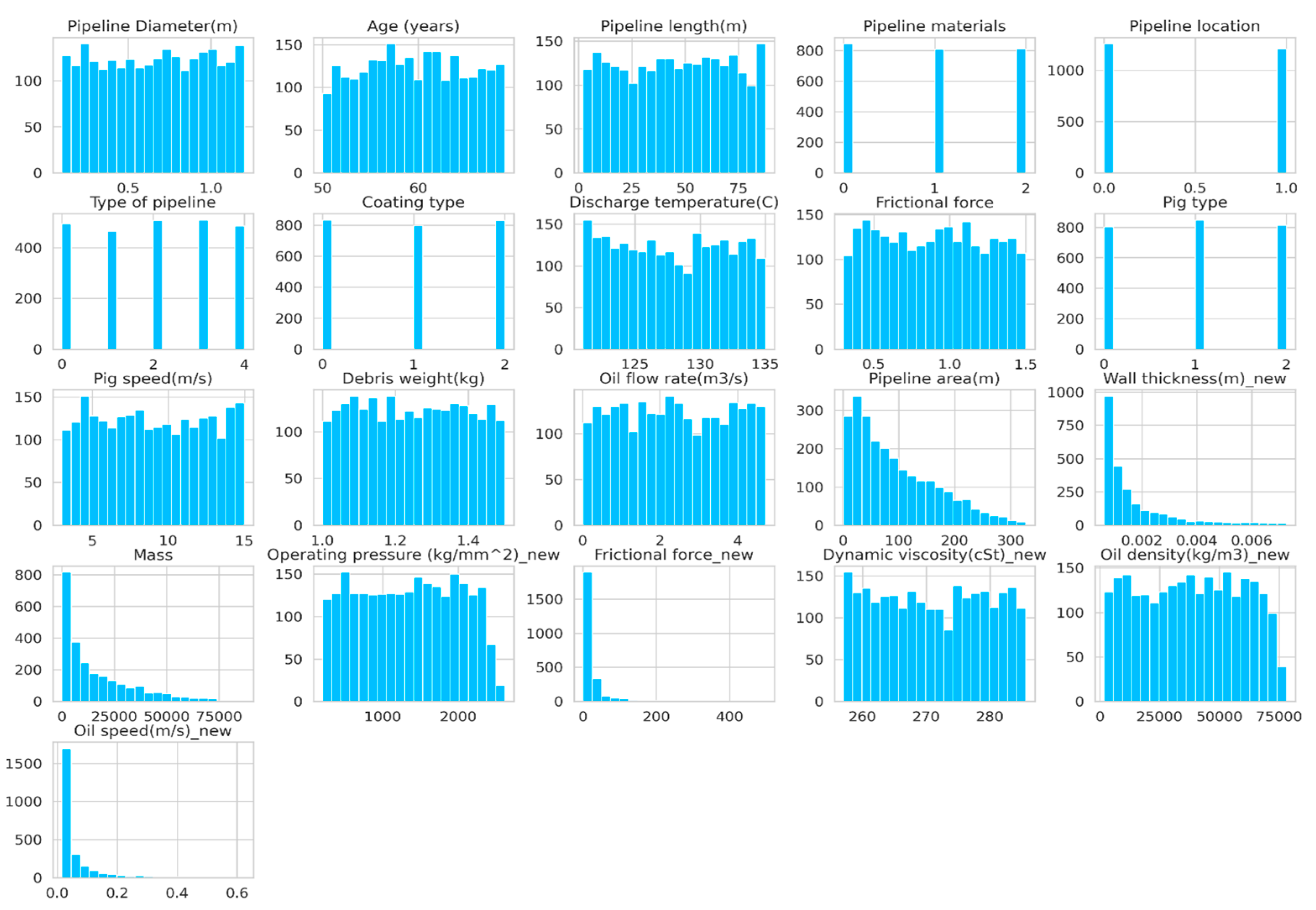
3.1. Pipeline Parameters Data Visualization
Histograms are a visual tool used to depict the distribution of a single variable. They display the frequency or count of data points within distinct intervals. Adjusting the number of bins allows for control over the level of detail in the representation. Choosing more bins increases detail but may make interpretation more complex, whereas fewer bins could oversimplify the distribution.
Figure 2 shows the data patterns of specific features (variables).
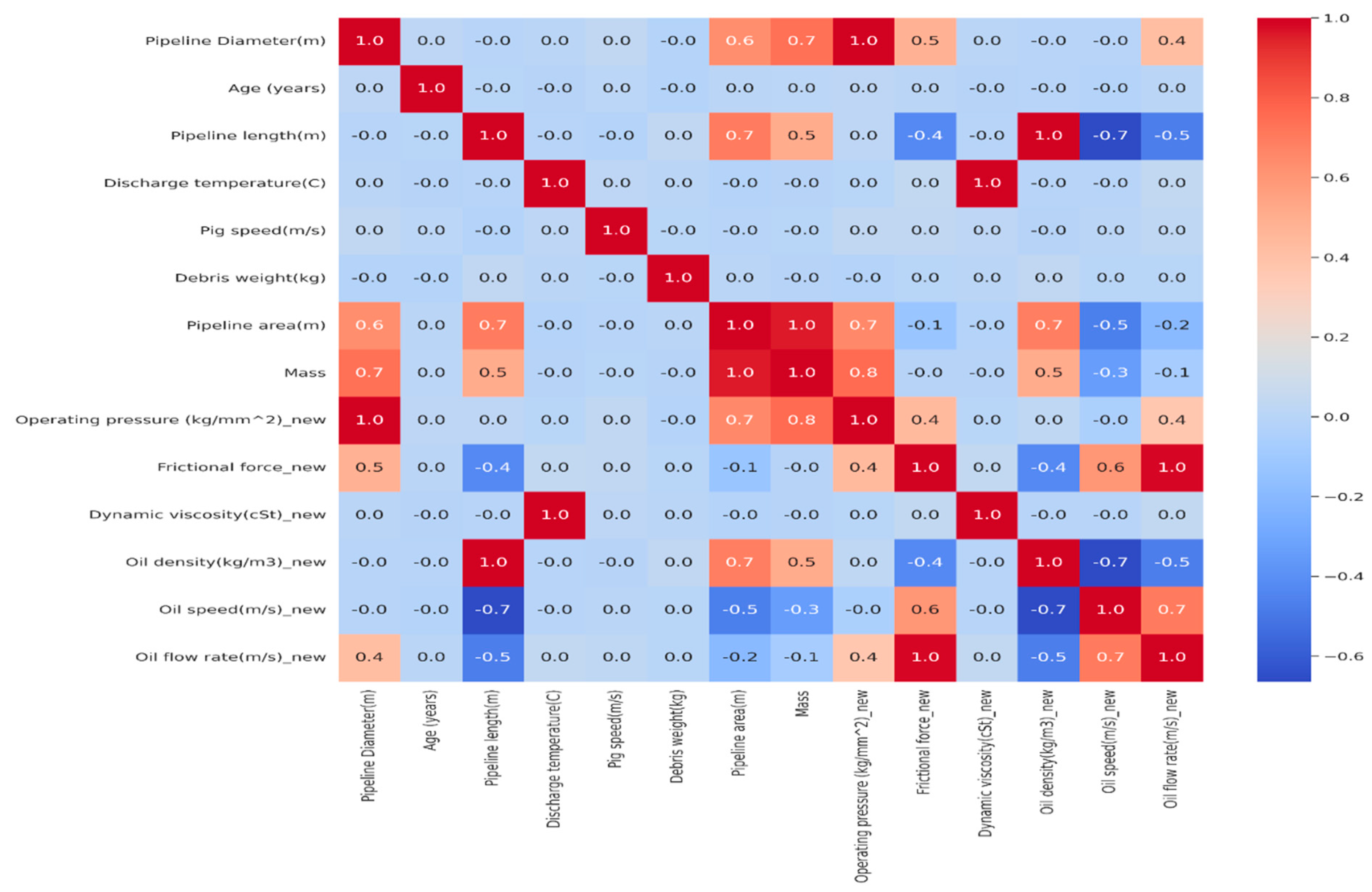
3.2. Correlation Matrix
The heatmap in
Figure 3 provides a visual assessment of the relationship among variables within the dataset. Intense colors indicate strong correlations, whether positive or negative, while lighter colors or shades of grey denote weaker correlations. Detecting patterns in variable associations, identifying multicollinearity issues, and prioritizing futures for further analysis or modeling are all made possible by heatmap analysis. Additionally, the annotation of correlation coefficient values provides accurate numerical information, improving the precision of interpretation and decision-making.
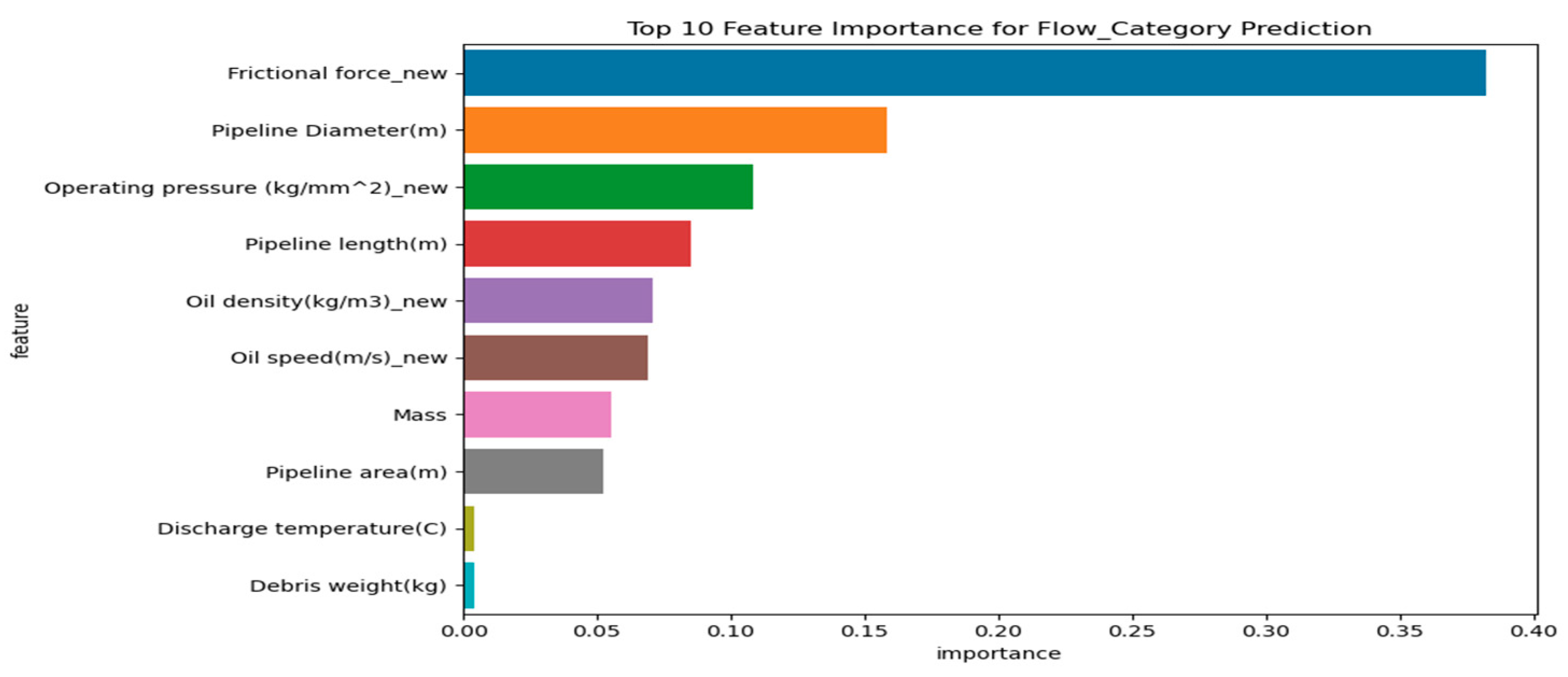
3.3. Feature Importance Analysis
The bar plot in
Figure 4 provides a visual representation of the importance of each feature in predicting the regression output. Features situated higher on the
y-axis are considered more influential in forecasting the target variable, whereas those positioned lower contribute less significantly. The length of each bar indicates the relative importance of its corresponding feature. The plot serves to highlight the significance of individual features within the regression model. This analysis facilitates the selection of features and comprehension of the underlying dataset relationships, potentially improving the model’s performance by prioritizing the most relevant features.
3.4. Linear Regressor Model Performance
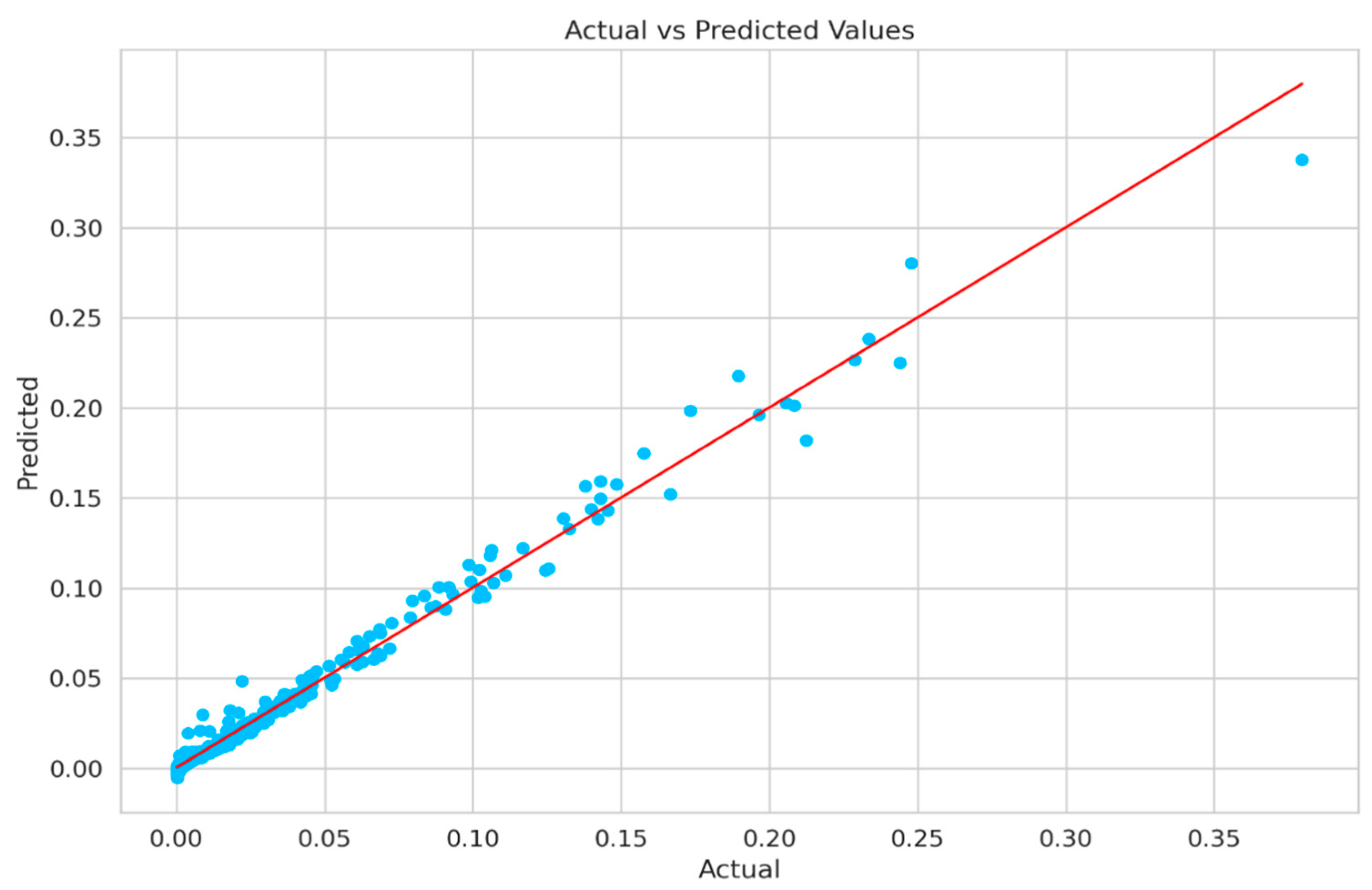
Figure 5 shows the plot of actual vs. predicted values of oil flow rate. The plot serves as a visual gauge for the model’s predictive performance and the extent of the linear relationship between the variables. When the points in the scatter plot closely align with the best-fit line, it signals that the model’s predictions closely match the actual values, indicating a strong fit. Conversely, if the points are spread widely around the best-fit line, it suggests a less accurate fit, implying that the model’s predictions may not be as reliable. Hence, the scatter plot aids in evaluating both the accuracy of the model’s predictions and the strength of the linear relationship between the variables.
3.5. Assembled Models’ Technique Performance Metrics Comparison
Ensemble techniques combine prediction from various individual models to enhance overall effectiveness. Typical ensemble techniques encompass Gradient Boosting, XGBoost Regressor Random Forest, K-Nearest Neighbors, Linear Regression, Ridge, Decision Tree, Huber Regressor, AdaBoost Regressor, ElasticNet, Lasso, and Support Vector Regressor. In this study, the RMSE, MAE, and R
2 were used to assess the performance of different models, as shown in
Table 1. These metrics consist of MSE, RMSE, R
2, and MAE, which are commonly utilized to evaluate the regression model’s performance. Lower MSE, RMSE, and MAE values, along with higher R
2 values, typically indicate higher model performance [
27]. The evaluation’s result shows that Gradient Boosting and XGBoost Regressor emerge as the top-performing models, while the Support Vector Regressor indicates lower satisfactory performance.
3.6. Assembled Models Comparison Based on RMSE and R2 Scores
Figure 6 compares the R
2 scores of an ensembled machine learning model. Each bar in the chart indicates a different model, with the length of the bar showing its R
2 score, which measures how well the model makes predictions. Taller bars indicate better performance. This chart helps visualize how well various models explain the data, simplifying the process of selecting the most suitable one for a specific task or dataset. It aids in making informed decisions regarding the choice of machine learning model. This chart helps in making informed decisions about which machine learning model to use.
3.7. Comparison of Actual vs. Predicted Flow Rate
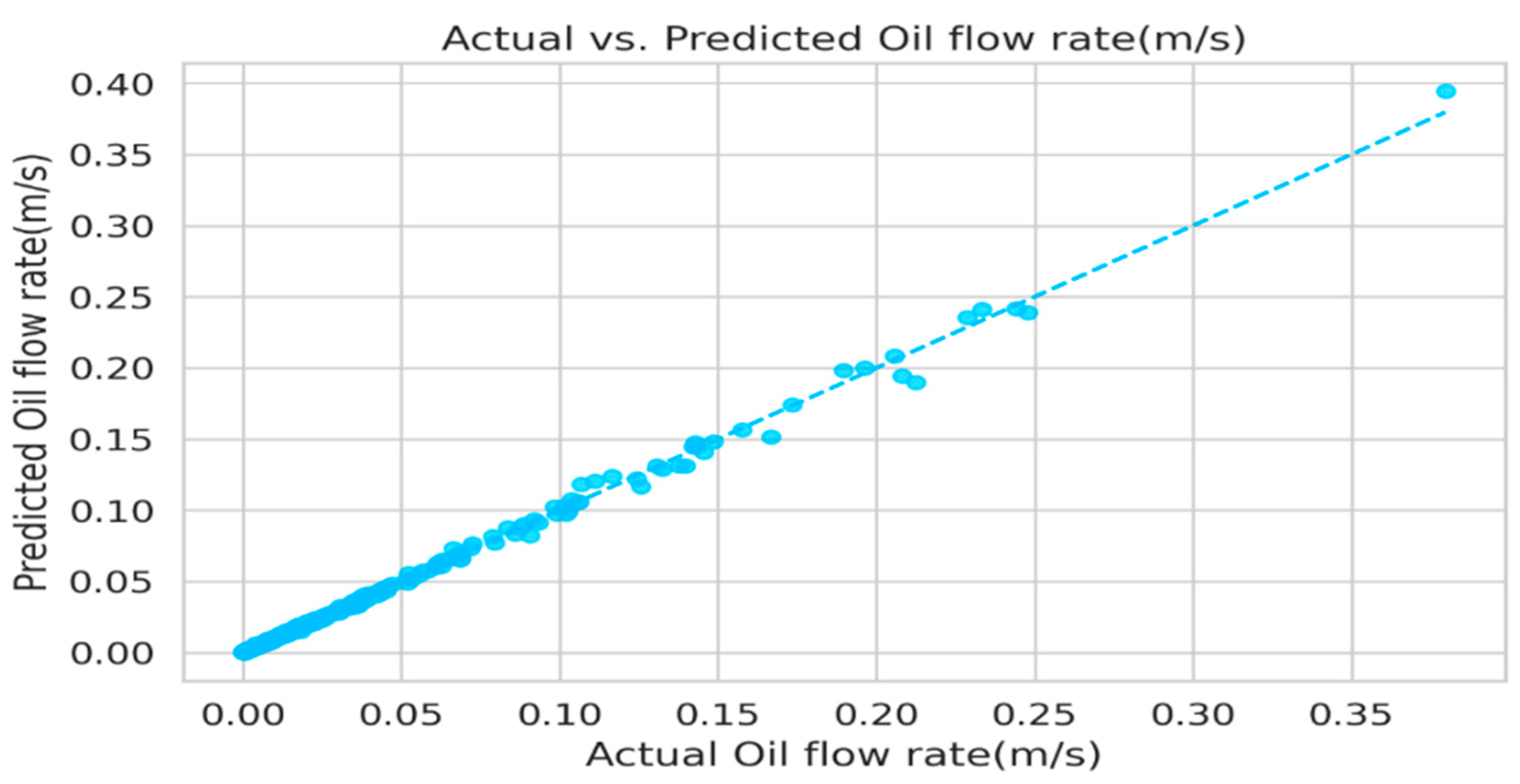
Figure 7 below shows the plot that presents a visual comparison between the predicted and actual flow rate, offering insights into the model’s predictive performance. Each data point represents a pair of predicted and actual values, with the
x-axis indicating the actual flow rate and the
y-axis representing the predicted ones. A dashed diagonal line serves as a reference for perfect alignment between predicted and actual values. Points above the line indicate overestimation, while those below suggest underestimation. The dispersion of points around this line indicates the level of agreement between actual and predicted values, with tighter clustering implying greater accuracy. This visual analysis aids in evaluating how well the model predicts flow rate, offering insights for possible adjustment to enhance its accuracy.
3.8. Optimized Maintenance Planning Using ML-Based Predictive Modelling
By analyzing real-time patterns in oil flow rate, the proposed ML model dynamically predicts maintenance needs in comparison to traditional maintenance strategies that depend on set schedules or predefined thresholds. By ensuring that maintenance is carried out in accordance with current pipeline conditions rather than static time-based plans, this data-driven method improves decision-making. This ML-based predictive model has the following benefits:
- (a)
Improved maintenance prediction accuracy: The model successfully predicts failure risks with high predictive accuracy (R2 = 0.997) by utilizing historical inspection data. Facilitating immediate interventions prior to significant performance loss enhances reliability.
- (b)
Optimized maintenance intervals: The model assigns three efficiency levels—High, Moderate, and Low—to pipeline flow rates, each of which is associated with a particular maintenance schedule. By minimizing unneeded interventions and ensuring that maintenance is only carried out when required, pipeline integrity is maintained.
- (c)
Reducing maintenance costs and downtime: The model improves overall pipeline performance and decreases operational costs and downtime by reducing needless maintenance tasks. This results in more effective resource allocation.
By supporting proactive maintenance planning and extending pipeline service life, this ML-driven approach offers a more flexible and economical option than traditional maintenance methods.
3.9. Comparison of Traditional and ML-Based Maintenance Approaches
A comparison between the proposed ML-based predictive maintenance model and traditional maintenance techniques is shown in
Table 2.
- (a)
Accuracy in Prediction
Since predictive accuracy metrics are not used by traditional maintenance techniques like Time-Based Maintenance (TBM), Condition-Based Maintenance (CBM), and Reliability-Centered Maintenance (RCM2), it can be challenging to make direct performance comparisons. When compared with the machine learning-based predictive model, it shows high predictive accuracy, with the Gradient Boosting algorithm achieving an R2 of 0.997. The higher performance highlights its capability to predict risks of failure with greater precision than expert-driven maintenance planning.
- (b)
Maintenance Frequency
TBM follows a fixed maintenance schedule and requires interventions 4–6 times per year [
28]. CBM decreases the maintenance frequency to 2 to 4 times per year by incorporating sensor-based monitoring but still relies on predefined thresholds and manual assessments [
29]. RCM2 also optimizes maintenance by risk-based assessment integration, resulting in 1 to 3 maintenance cycles per year; however, it also depends on expert judgment when making decisions [
30]. In contrast, the machine learning-based predictive maintenance model minimizes interventions 1 to 2 times per year by adjusting schedules dynamically based on real-time conditions of the pipeline and ensuring efficiency without compromising reliability.
- (c)
Cost Efficiency
Because of its strict scheduling method, TBM does not provide savings in costs. CBM and RCM2 reduce unnecessary maintenance activities, which results in moderate cost savings (10–25%). Because it optimizes resource allocation, minimizes operating expenses, and dynamically schedules maintenance only when necessary, the ML-based predictive maintenance strategy provides the best cost efficiency, with potential savings of 30–50% [
31].
- (d)
Downtime Reduction
In traditional methods, unscheduled maintenance and pipeline failures are major causes of downtime. By predicting and proactively addressing possible issues before they worsen, the ML-based method prevents unplanned shutdowns and increases overall system availability, reducing downtime by 40–50% [
31].
- (e)
Failure Prevention Efficiency
Due to their reliance on rigid schedules or expert-driven risk assessments, traditional maintenance strategies have failure prevention rates of between 50 and 80%. By continuously analyzing variations in oil flow rates to identify early indicators of deposit formation and other irregularities, the machine learning (ML)-based predictive maintenance model achieves 90–95% efficiency, greatly improving failure prevention. This feature ensures a proactive maintenance plan that successfully reduces operational risks [
15,
32].
4. Conclusions
The study analyzes how well machine learning models can predict the need for maintenance to be carried out in oil pipelines, specifically examining the rate of fluid travel through the pipelines. The study reveals that employing these models, trained on inspection data, can accurately predict oil flow rate in pipelines, thereby assisting in maintenance planning. A change in flow rate indicates the potential buildup of blockages in the pipes, suggesting that maintenance is needed. A higher oil flow rate indicates that the system is functioning well and that there is no need to carry out maintenance and can be postponed, whereas a slower flow rate provides a signal that there is a problem like a buildup of deposits within the pipeline; thus, maintenance is needed. Variable performance levels among the ensemble models were observed. Notably, Gradient Boosting and XGBoost Regressor indicate the highest accuracy, exhibiting better predictions and lower error rates compared to the Support Vector Regressor. Gradient Boosting shows an MSE of 0.000005, an RMSE of 0.002259, an MAE of 0.000968, and an R2 of 0.997259. Similarly, XGBoost Regressor had an MSE of 0.000005, an RMSE of 0.002269, an MAE of 0.000922, and an R2 of 0.997234. The Support Vector Regressor showed lower performance with an MSE of 0.002868, RMSE of 0.053554, MAE of 0.046311, and an R2 of −0.540765. The study findings emphasize the importance of selecting a suitable machine learning model that aligns with the available dataset task objectives. They also illustrate how professionals in the oil and gas industry can use these insights to make informed decisions in using machine learning for scheduling maintenance in oil pipelines. This approach improves maintenance practices within the oil and gas industry by using predictive models. Further study and validation are needed to enhance these findings and advance the techniques of predictive maintenance in the industry.


