Evaluation of Seismic Effects on Atmospheric Pressure Liquid Storage Tanks ^†

Abstract

As part of the seismic capacity assessment of thin-walled tanks containing liquid fuels, the appropriate modeling of hydrodynamic loads is required. The theory adopted in existing work requires the modeling of the hydrodynamic pressure contribution due to tank deformability, which, however, cannot be calculated in closed form. The approach adopted in this work uses acoustic–structural modal analysis to obtain the deformation and response period required to calculate this contribution. The use of the proposed method, on a finite element model, allows the implementation of thickness variability and more geometric detail in the modal analysis. On the other hand, using the obtained load distributions, in non-linear static analyses, reduces the computational time compared to dynamic simulations. In addition, analyses can be performed by importing a pre-deformed surface derived from a three-dimensional scan of the real tank into the final model, thus including the effect of geometric imperfections. As a case study, an existing tank model was produced and analyzed, and the same damage patterns documented in real cases following seismic events were obtained. Therefore, due to the low computational cost, this method is appropriate to be reproduced for a statistically significant number of load cases.

1. Introduction

The evaluation of the seismic vulnerability of structures used to contain liquids (tanks) is an area of study that is of primary importance not only for the safety and security of people in proximity to such structures but also for the appropriate operation of the utilities and facilities of which such structures may be a part.

Neglecting, momentarily, the interaction between the bottom and the shell, if H is the wetted height by the fluid, R is the radius of the cylindrical tank, and z is the height at which the tension is picked up $\sigma \theta \left(z\right)$, with one of the two principal radii of curvature being infinite and the other equal to R, we have membrane equilibrium

$$p=\rho g(H-z)={\displaystyle \frac{N_{\theta }}{R}}\Rightarrow {\sigma }_{\theta }={\displaystyle \frac{N_{\theta }}{s}}={\displaystyle \frac{\rho gR(H-z)}{s}}$$

(1)

where s is the thickness of the cylindrical shell, $g\rho$ is the specific gravity of the contained liquid, and $N_{\theta }$ is the circumferential stress per unit length. Consequently, if we desire constant tension, we must vary the thickness with the elevation by increasing it back toward the base of the tank.

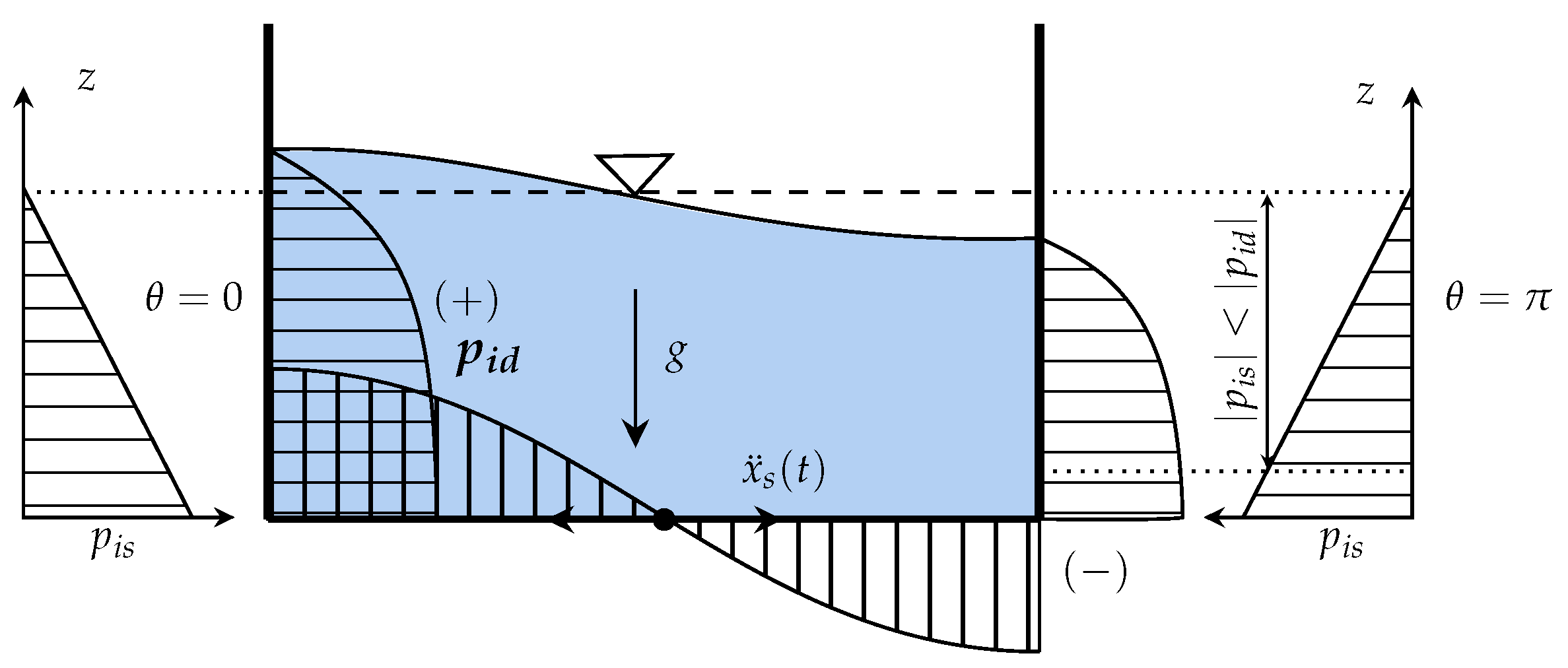
1.1. Seismic Stress Modeling

The evaluation of seismic effects is dependent on the choice of a measure of the earthquake intensity. Examples of such measures are the peak ground acceleration (PGA) and the value of the elastic response spectrum corresponding to the fundamental period of the structure ($S_e\left(T_1\right)$).

Alternatively, it is possible to use a group of accelerograms, recorded at different locations, whose values are scaled by appropriate safety coefficients to obtain accelerograms called spectra-compatible accelerograms. In this way, it is possible to obtain response spectra that have the characteristic pattern of a real seismic event and values compatible with those obtained from the norm, as shown in Figure 1.

1.2. Seismic Damage Characteristics

The seismic damage modes for cylindrical atmospheric pressure vessels are numerous and are not all easily identifiable; in this paper, we assume that these mechanisms are dependent on the inertial effects given by the mass of liquid contained.

To this hydrodynamic pressure field $p_{id}(x,t)$ is added the hydrostatic field $p_{is}\left(z\right)$ (Figure 2). The occurrence of this new asymmetric loading condition is the main cause of the local instabilities responsible for shell damage, two of the most frequent of which can be listed as follows.

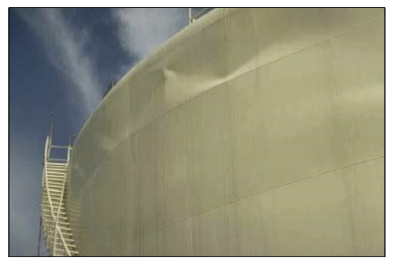
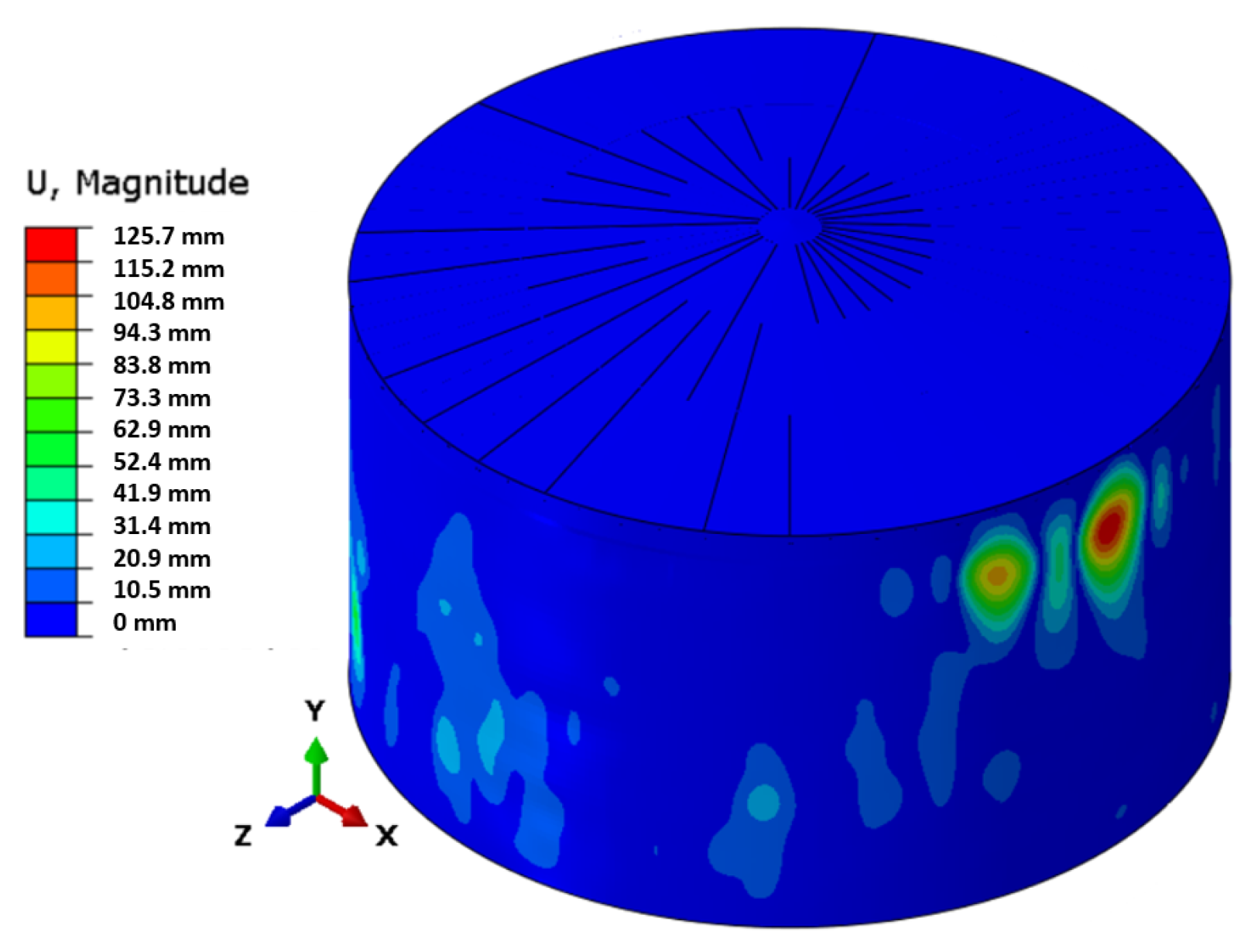
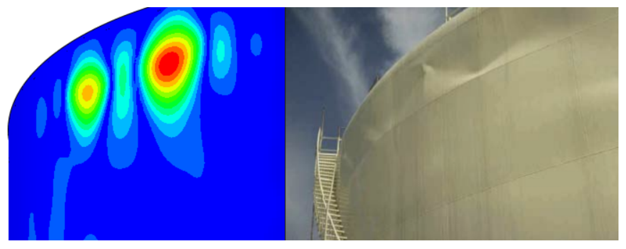
• Buckling in the upper portion of the shell (top buckling): if the depression due to the hydrodynamic effect is excessive, the tank may collapse inwards (Figure 3).
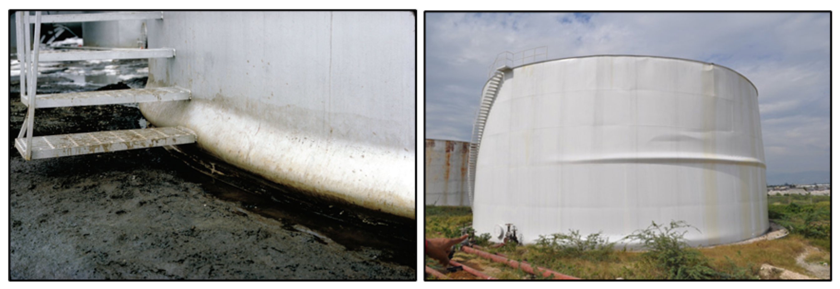
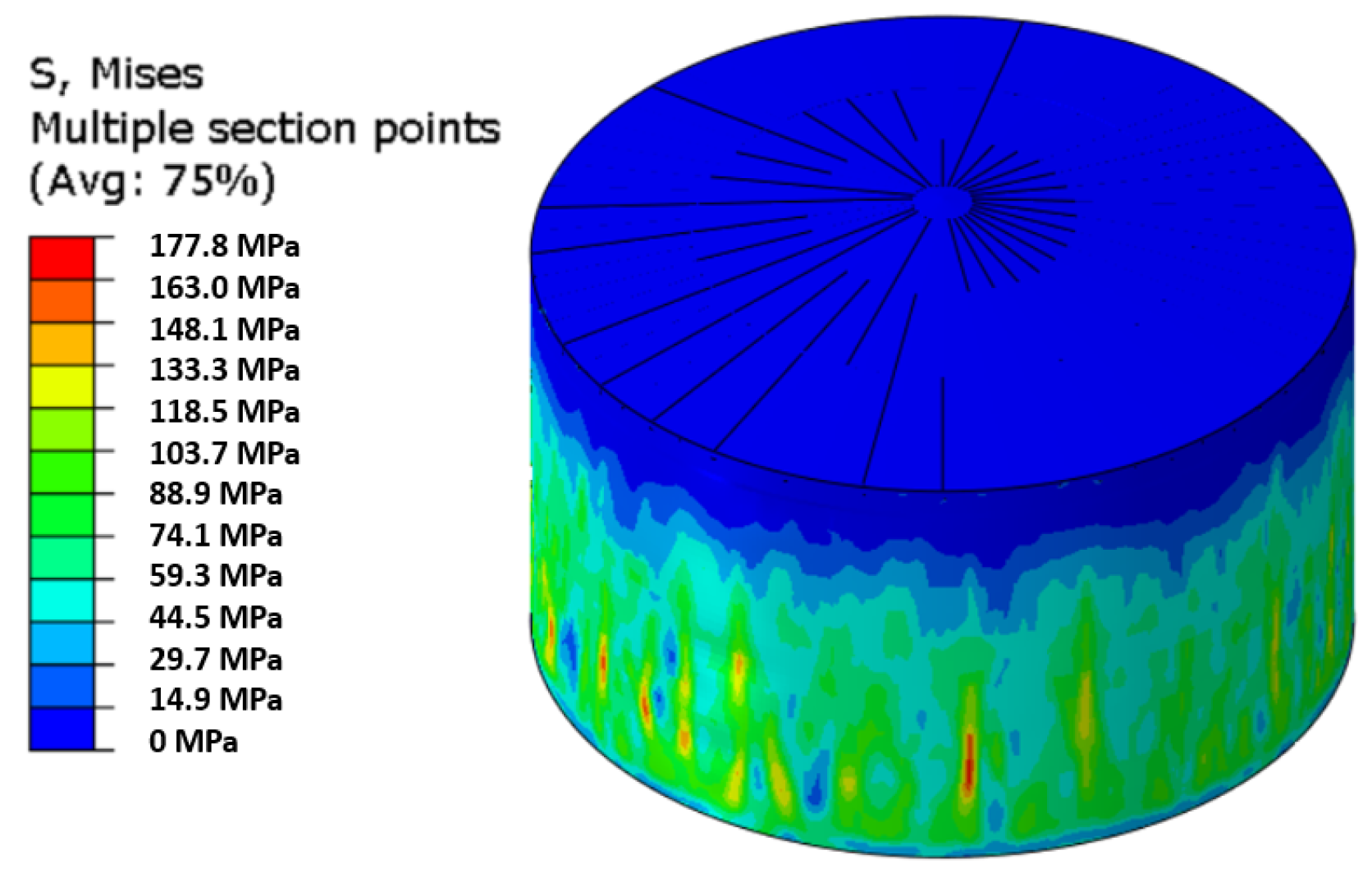
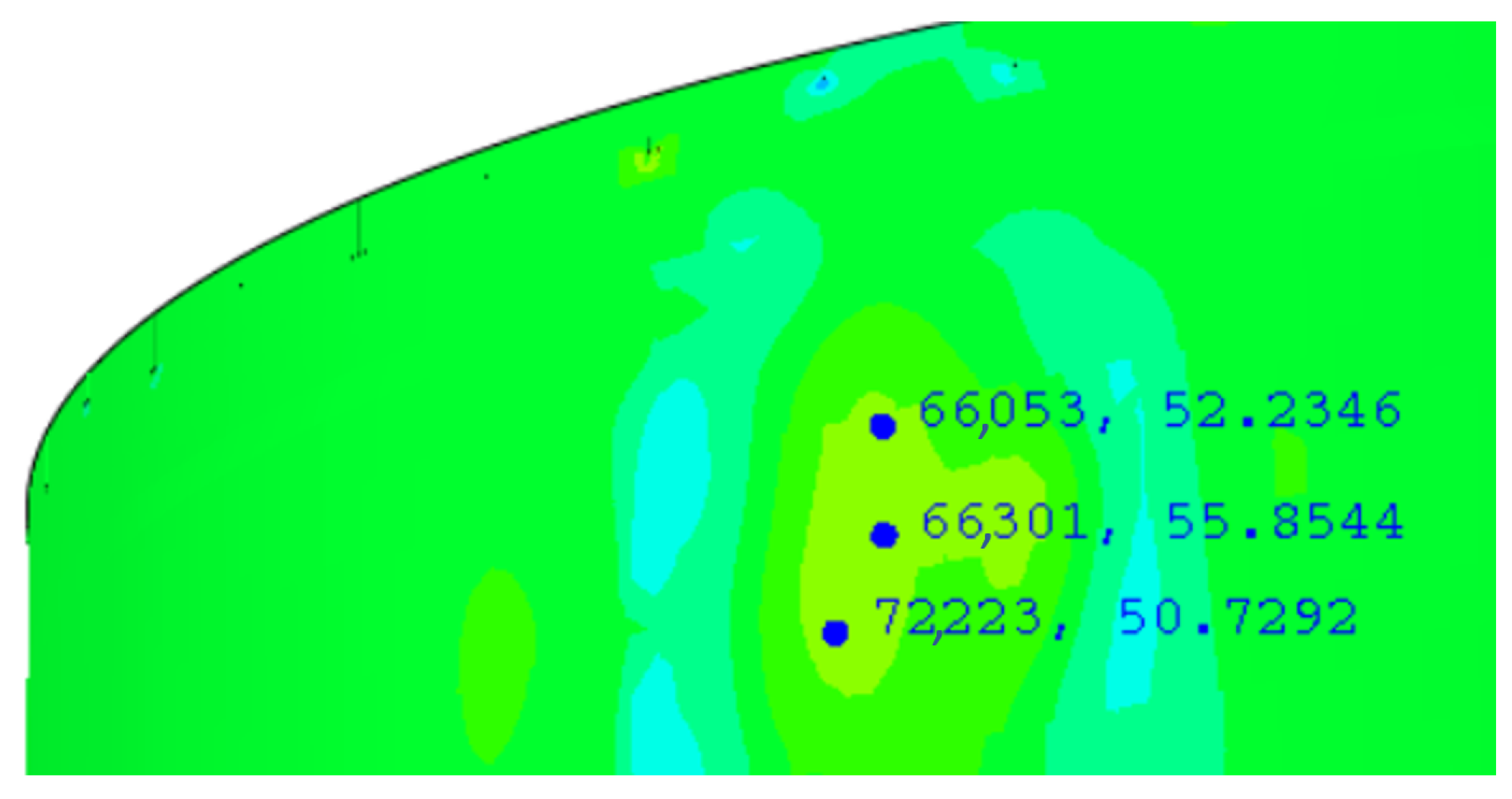
• Instability in the lower portion of the tank: if the overpressure due to hydrostatic loading and the hydrodynamic effect exceeds the yield strength of the material, even if the course is mainly stressed still in the plane (as a membrane), there is excessive deformation due to plasticization, which, with the effect of axial stress, can lead to instability. This damage is usually called elephant foot (Figure 4).

1.3. Reference Norms

The design and verification of tanks is an activity regulated by local regulations. In this work, we refer mainly to Eurocode 8 Part 4 (EC8 Part 4) for the modeling and application of hydrodynamic loads. We also refer to the Turkish (TBDY 2018) standard [1] for the calculation of the spectra from the standard and the related multiplicative coefficients used to scale the values of the response spectra.

2. Eurocode 8 Theoretical Bases—Part 4

The norm first requires the use of a rational method, based on the solution of hydrodynamic equations with appropriate boundary conditions, to evaluate the response of the tank system to seismic action.

In detail, effects regarding the convective component are separated from the impulsive component of liquid motion. The fluid is considered to be incompressible.

2.1. Seismic Analysis Procedures for Tanks (Annex A)

The theory adopted is the linear velocity potential framework, reworked by Jacobsen and Housner [2,3,4] for more intuitive application in structural seismic analysis.

Housner’s model reduces the motion of the fluid inside the tank to a system of concentrated masses connected to the tank by springs with different stiffness. There are two contributions that constitute the motion field and thus the hydrodynamic pressure field:

• the impulsive contribution;
• the convective contribution.

This differentiation appears as a consequence of the combined application of the hypotheses of incompressible, irrotational, and inviscid flows and the hypothesis of small oscillations to the equations of motion, i.e., the following system:

$$\{\begin{array}{l}\rho \frac{\partial \mathbf{V}}{\partial t}+\rho (\mathbf{V}·\nabla )\mathbf{V}=-\nabla p-\rho {\ddot{x}}_s\left(t\right)·{\mathbf{e}}_x-\rho g·{\mathbf{e}}_z\\ \nabla ·\mathbf{V}=0\\ \nabla \times \mathbf{V}=\mathbf{0}\iff \mathbf{V}(\mathbf{x},t)=\nabla \mathrm{\Phi }\end{array}$$

(2)

In detail, the assumption of irrotationality (the last instance in (2)) is mathematically equivalent to assuming the existence of a velocity scalar potential $\mathrm{\Phi }(\mathbf{x},t)$. Using this assumption with the second component of (2), the Laplace equation (3) is obtained:

$$\nabla ·\mathbf{V}=\nabla ·(\nabla \mathrm{\Phi })={\nabla }^2\mathrm{\Phi }=0$$

(3)

The field of motion (Figure 5) can be solved for the complete system of an infinitely rigid tank by superposing two characteristic solutions of the Laplace equation given by two different sets of boundary conditions:

$$\left\{\begin{array}{l}{\nabla }^2\mathrm{\Phi }=0\\ \mathrm{\Phi }(\mathbf{x},0)=0& \mathrm{per}t=0\\ {\left(\frac{\partial \mathrm{\Phi }}{\partial t}\right)}_{t=0}=0& \mathrm{per}t=0\\ \nabla \mathrm{\Phi }·\mathbf{n}=-{\dot{x}}_s\left(t\right)cos\theta & \mathrm{su}r=R\\ \frac{\partial \mathrm{\Phi }}{\partial t}=0& \mathrm{su}z=H\end{array}\right\{\begin{array}{l}{\nabla }^2\mathrm{\Phi }=0\\ \mathrm{\Phi }(\mathbf{x},0)=0& \mathrm{per}t=0\\ {\left(\frac{\partial \mathrm{\Phi }}{\partial t}\right)}_{t=0}=0& \mathrm{per}t=0\\ \nabla \mathrm{\Phi }·\mathbf{n}=0& \mathrm{su}r=R\\ {\displaystyle \frac{1}{g}}\frac{{\partial }^2\mathrm{\Phi }}{\partial t^2}=-{\displaystyle \frac{{\stackrel{⃛}{x}}_s}{g}}x-\frac{\partial \mathrm{\Phi }}{\partial z}& \mathrm{su}z=H\end{array}$$

(4)

The first group of conditions in (4) gives the contribution called rigid impulsive; the second group of conditions in (4) gives the contribution called convective.

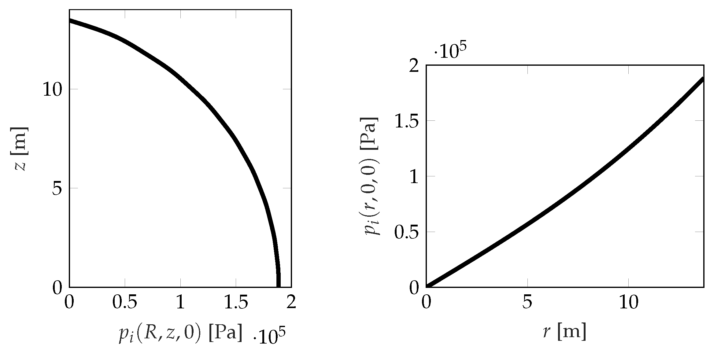
2.2. Rigid Impulsive Component

The impulsive potential returns a hydrodynamic pressure distribution, which, in EC8 Part 4, is expressed through Equation (5):

$$p_i(\xi ,\zeta ,\theta ,t)=C_i(\xi ,\zeta )\rho Hcos\theta A_g\left(t\right)$$

(5)

where $\xi =r/R$; $\zeta =z/H$ and where the coefficient $C_i(\xi ,\zeta )$ is given by

$$C_i(\xi ,\zeta )=2\sum _{n=0}^{\infty }{\displaystyle \frac{{(-1)}^n{I}_1\left(\frac{{\nu }_n}{\gamma }\xi \right)}{I_1^{\prime }({\nu }_n/\gamma ){\nu }_n^2}}cos\left({\nu }_n\zeta \right)$$

(6)

with ${\nu }_n=(2n+1)\pi /2$ and $\gamma =H/R$.

$I_1(·)$ is the Bessel function of the first kind and $I_1^{\prime }(·)$ is its derivative.

In Figure 6, the dimensionless impulsive pressure distribution on the wall and bottom for an infinitely rigid tank is reproduced.

Because, through (5), the impulsive pressure is a computable analytical expression, the calculation of the impulsive shear action $Q_i$ and impulsive overturning moment $M_i$ by numerical or analytical integration is possible; however, the norm already provides closed-form results for impulsive masses and heights:

$$m_i=m2\gamma \sum _{n=0}^{\infty }{\displaystyle \frac{I_1({\nu }_n/\gamma )}{I_1^{\prime }({\nu }_n/\gamma ){\nu }_n^3}}$$

(7)

where $m=\rho \pi R^{2}H$ is the total mass of the contained fluid.

Therefore, we have

$$Q_i\left(t\right)=m_i·A_g\left(t\right)$$

(8)

Similarly, we have the impulsive heights, related to the integrated pressure multiplied by the $\zeta$ coordinate, on the tank wall ($h_i$):

$$h_i={\displaystyle \frac{H·m}{m_i}}\sum _{n=0}^{\infty }{\displaystyle \frac{{(-1)}^n{I}_1({\nu }_n/\gamma )}{{\nu }_n^4·I_1^{\prime }({\nu }_n/\gamma )}}({\nu }_n{(-1)}^n-1)$$

(9)

Of course, this results in

$$M_i\left(t\right)=m_i·h_i·A_g\left(t\right)$$

(10)

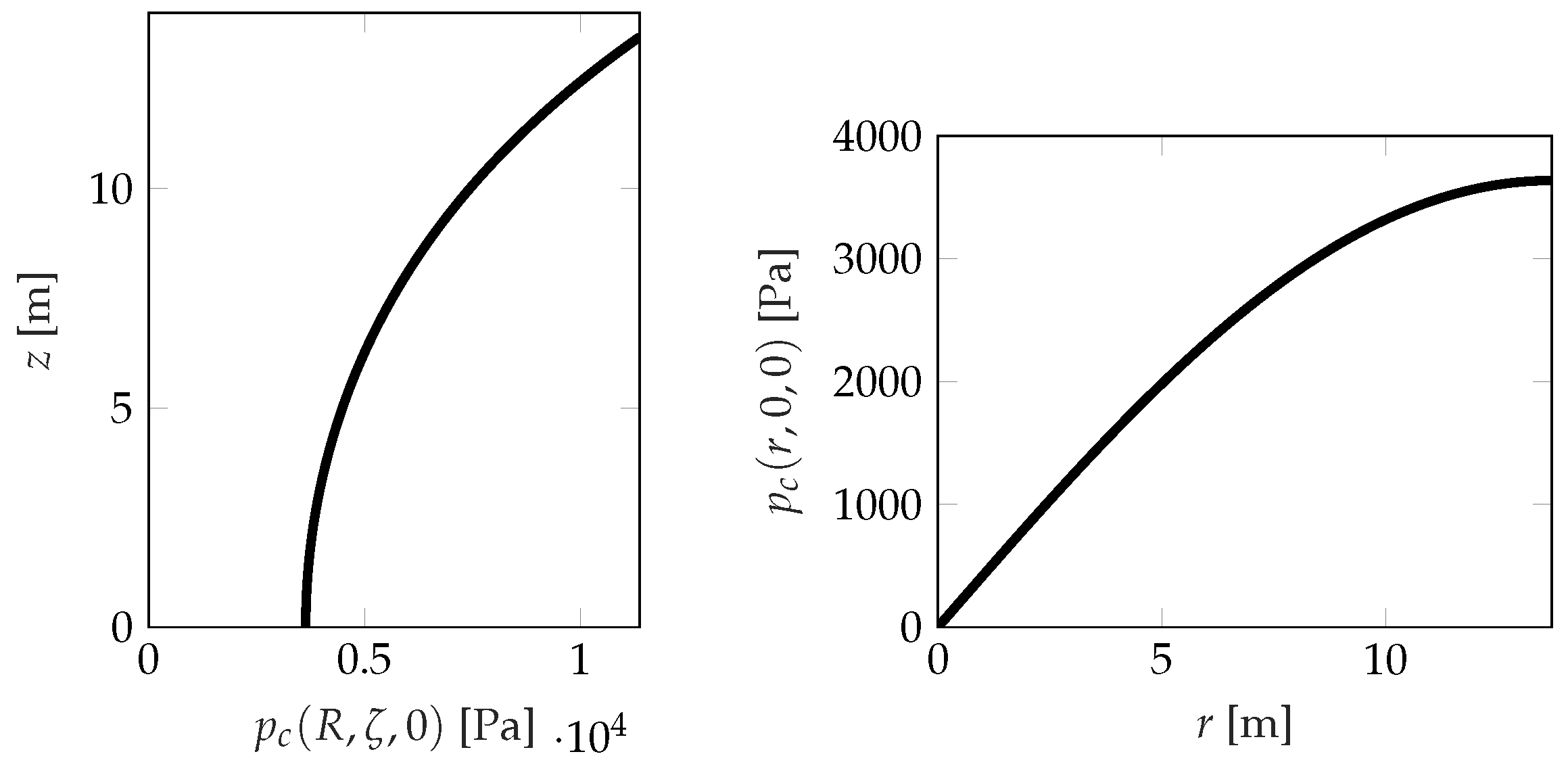
2.3. Convective Contribution

For this pressure contribution, the solution of the Laplace equation with the second set of boundary conditions (4) returns the following relation:

$$p_c(\xi ,\theta ,\zeta ,t)=\rho \sum _{n=1}^{\infty }{\psi }_{n}cosh\left({\lambda }_n\gamma \zeta \right)J_1\left({\lambda }_n\xi \right)cos\theta A_{c,n}\left(t\right)$$

(11)

where every term ${\psi }_n$ is given by

$${\psi }_n={\displaystyle \frac{2R}{({\lambda }_n^2-1)J_1\left({\lambda }_n\right)cosh\left({\lambda }_n\gamma \right)}}$$

(12)

where $J_1(·)$ is a first-order Bessel function of the first kind and ${\lambda }_n$ are the values that satisfy the condition $J_1^{\prime }\left({\lambda }_n\right)=0$. The $A_{c,n}\left(t\right)$ acceleration components of the convective modes correspond to the response of a single-degree-of-freedom oscillator with the following circular frequency:

$${\omega }_{c,n}=\sqrt{g{\displaystyle \frac{{\lambda }_n}{R}}tanh\left({\lambda }_n\gamma \right)}$$

(13)

Figure 7 shows the convective pressure distribution plots.

2.4. Solution Method Considerations

In order to solve the modal problem and obtain the circular frequency of the flexible–impulsive component required for the complete calculation of the seismic actions, the EC8 Part 4 norm recommends using the iterative procedure of Fischer and Rammerstorfer [5]. According to this approach, an added density can be calculated by attempting to apply deformation to the radial term of the mass matrix, proceeding with successive iterations.

With the formulation of the added density, a singularity is introduced at the base, with the boundary condition $f(\zeta =0)=0$. This singularity, even with the simplifying assumption of keeping the thickness constant, can be solved by numerical methods, but this involves additional effort and computational resources.

Fischer et al., in a later review, no longer mention the iterative method and suggest the use of a simplified approach with deformation approximated by a sine or cosine function [6].

It can be seen that both the semi-analytical method outlined by Habenberger and the iterative method proposed by Fischer and Rammerstorfer entail various complications in practical use, due to the limitations in assuming a regular geometry and the programming work required to set up the appropriate calculation codes.

In the literature, there are various examples of numerical models that try to reproduce fluid–structural interactions using various methods; in particular, the ones that return the most accurate results are based on finite element analysis.

These include the arbitrary Eulerian Lagrangian (ALE) method [7,8,9,10], analyses based on computational fluid dynamics (CFD) models [7,11,12], particle methods such as smoothed particle hydrodynamics (SPH) [13,14], and acoustic element methods [15,16,17,18].

3. Deformable Tanks

This discussion refers to linear potential theory under the assumption of an infinitely rigid tank in order to greatly simplify the calculation of the pressure distributions and to make it possible to obtain closed-form expressions of the potential.

Paragraph 3 of Annex A of the EC8 Part 4 norm describes the procedure for the evaluation of the effects of hydrodynamic action caused by tank wall deformability. With a conservative approach, the norm assumes that these effects are to be considered separately from the effects already seen and therefore suggests their combination in different ways.

However, the component due to flexibility that is to be considered will be related only to impulsive effects and not to convective effects, as a consequence of the evident distance between the values of the cylindrical shell’s frequency range and the liquid mass oscillations (the convective effect) [5,19,20].

The relationship provided in EC8 requires knowledge of the radial deformation along the height associated with the impulsive loading of the fluid–structural system, i.e., the first antisymmetric deformation mode of the fluid-coupled shell. The deformability of the shell directly affects the hydrodynamic pressure distribution; this problem is non-linear and can only be approached numerically or by iterative means.

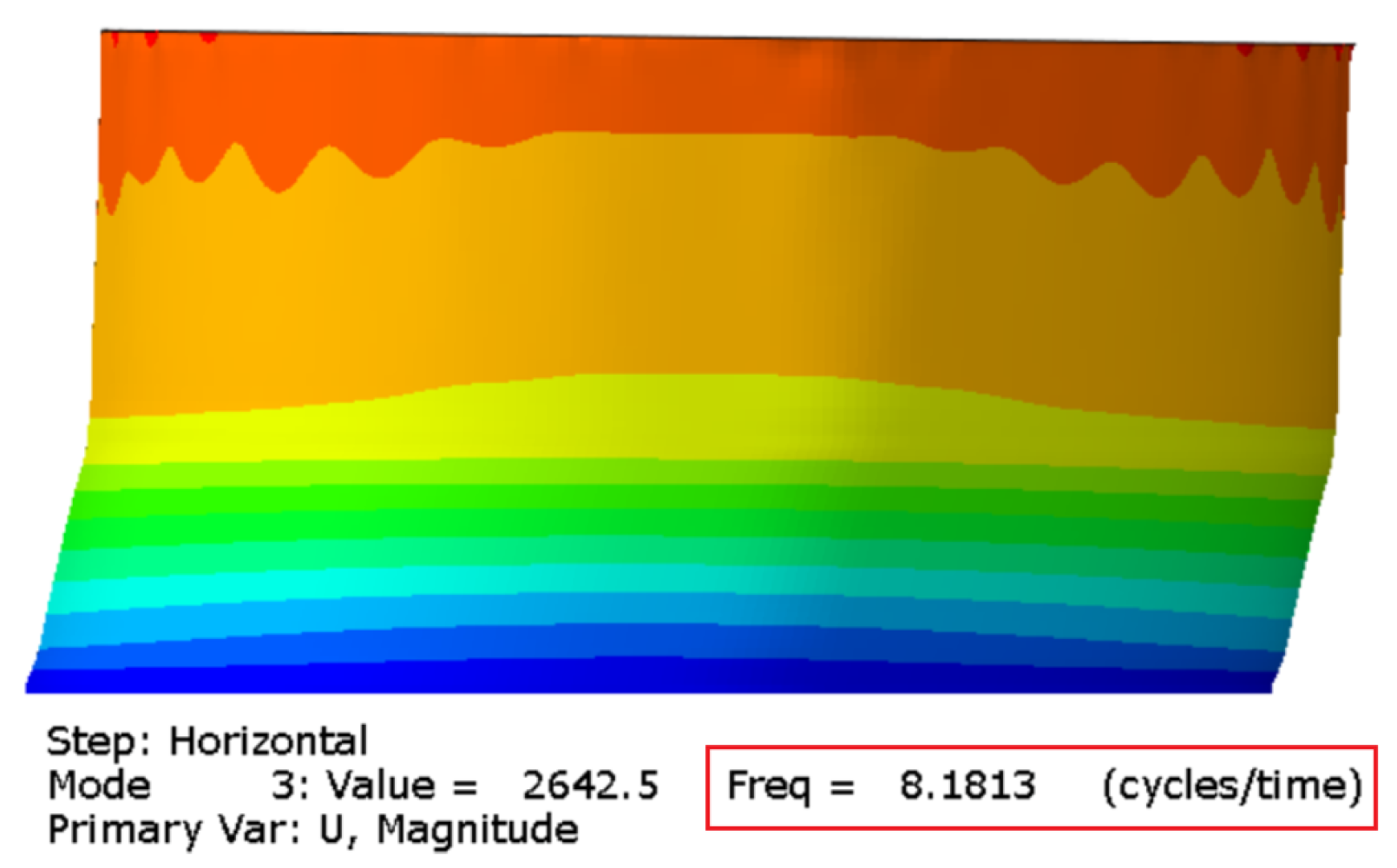
3.1. Fluid–Structural Modal Analysis

To obtain the coupled oscillation modes, it is necessary to set up the dynamic problem and obtain the corresponding modal problem, i.e., the study of free oscillations, of the fluid–structure system.

To obtain the dynamic system, the static problem must be addressed via the inertial actions of the shell and the external loads. Denoting by $\mathbf{U}$ the vector of displacement, $\mathbf{p}$ the vector of known loads, and $\left[S\right]$ the stiffness matrix of the tank obtainable from the flexural theory of asymmetrically loaded shells [21], we obtain

$$\left[S\right]\mathbf{U}-{\displaystyle \frac{R^2}{K}}\left[M\right]\frac{{\partial }^2\mathbf{U}}{\partial t^2}={\displaystyle \frac{R^2}{K}}\mathbf{p}$$

(14)

Because we are only interested in the mode of oscillation of the coupled system, we consider only the hydrodynamic action on the walls, neglecting, at this stage, the inertial forces of the shell, the hydrostatic pressure, and the vertical and circumferential forces. Therefore, the only non-zero load component is $p_r=p_{i,f}(\xi ,\theta ,\zeta ,t)$, the impulsive hydrodynamic pressure that also takes into account the deformability of the walls. The formulation of this is also derived from potential theory:

$$p_{i,f}(\xi ,\theta ,\zeta ,t)=-\rho \frac{\partial {\mathrm{\Phi }}_{i,f}}{\partial t}$$

(15)

The boundary conditions for the potential are analogous to those adopted for the impulsive solution in the rigid tank case expressed by the first system in (4), but, in this case, the displacement $w\left(t\right)$ is the radial displacement of the tank wall relative to the base. The general solution of the impulsive potential returns for the impulsive hydrodynamic pressure in the case of flexible tanks has the following non-closed form:

$$p_{i,f}=-\rho H\mathrm{\Psi }\sum _{n=0}^{\infty }{\displaystyle \frac{{\displaystyle 2{\int }_0^1\left[f\left(\zeta \right)cos\left({\nu }_n\zeta \right)\right]\mathrm{d}\zeta }}{I_1^{\prime }({\nu }_n/\gamma ){\nu }_n}}{I}_1\left({\displaystyle \frac{{\nu }_n}{\gamma }}\xi \right)·cos\left({\nu }_n\zeta \right)A_{f,n}\left(t\right)·cos\theta$$

(16)

where the flexible acceleration is factorized into a set of modal terms $A_{f,n}$ and multiplied by a participation factor $\mathrm{\Psi }$ that takes into account the structural mass and the mass of the liquid, while the value of the integral is calculated with respect to a dimensionless modal form $f\left(\zeta \right)$. The axial mode of interest is always the one related to the single buckling of the axis line $n=1$.

If we approximate the deformation with a trigonometric function, such as sine, we would have $w(\zeta ,\theta )=f\left(\zeta \right)cos\theta =sin(\zeta \pi /2)cos\theta$ as the first mode; in this case, it is also possible to calculate the dimensionless pressure distribution as the tank characteristics vary using (16), as reproduced in Figure 8 for different values of the parameter $\gamma =H/R$.

A semi-analytical approach to solving the modal problem is given by Habenberger [22], who uses an integral formulation of the coupled modal problem. For the stiffness matrix $\left[S\right]$, Habenberger uses a simplified formulation, also devised by Flügge, which neglects the off-diagonal terms.

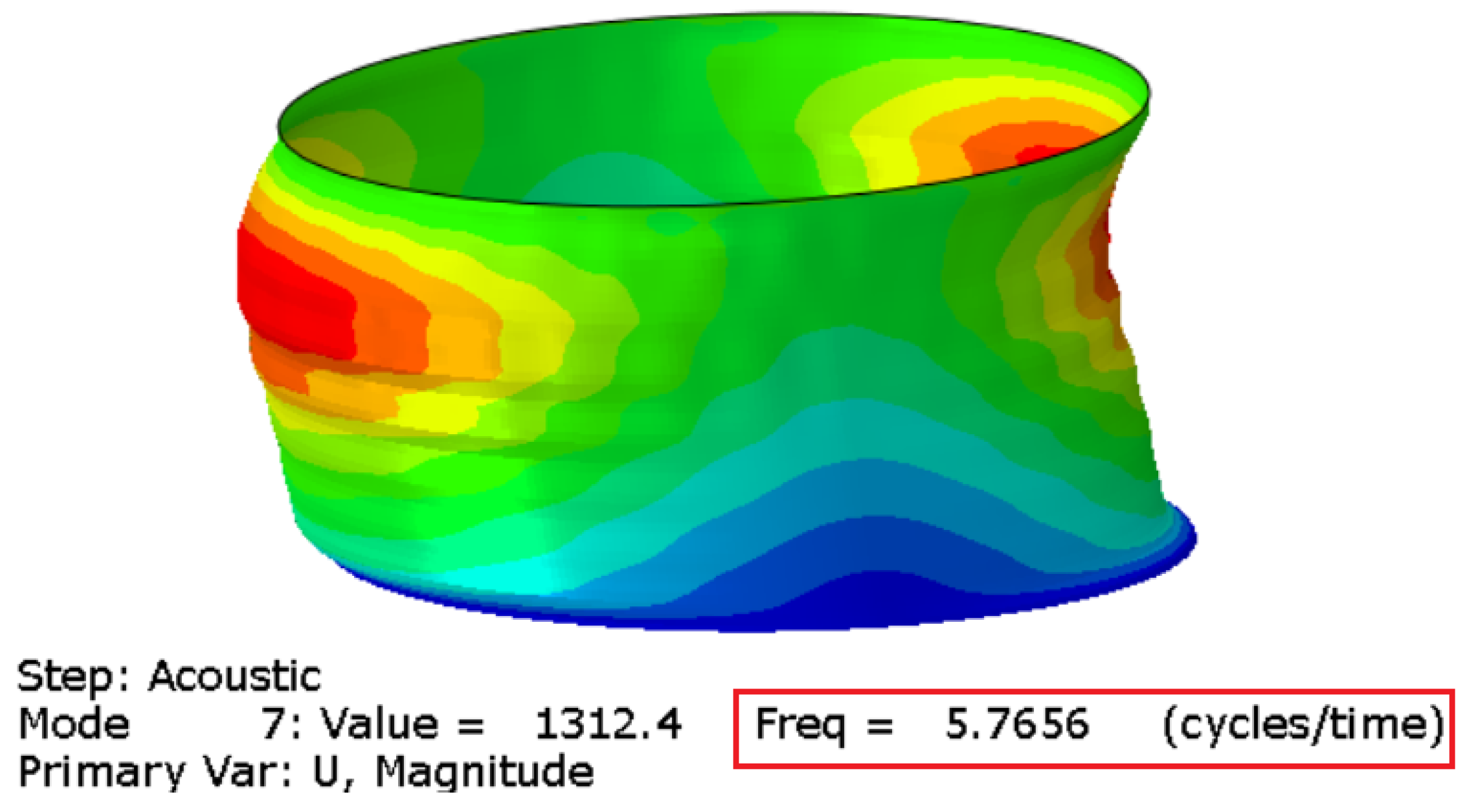
3.2. Acoustic Modal Analysis

In order to obtain the modal deformation $f\left(\zeta \right)$ and the corresponding circular frequency ${\omega }_f$ necessary for the complete calculation of the pressure distribution with (16), the coupled modal problem must be solved. The solution proposed in this work is obtained using the finite element method with an acoustic formulation of the fluid dynamic field coupled to the structural problem.

It is further assumed that the degrees of displacement u normal to the fluid–structural interface are shared by both the fluid and the structure, i.e., that there is always wall adhesion. Consequently, the solid elements representing the fluid domain will possess only one degree of freedom associated with the hydrodynamic pressure p.

With these assumptions, the coupled modal problem can be formulated to be solved with the Lanczos algorithm.

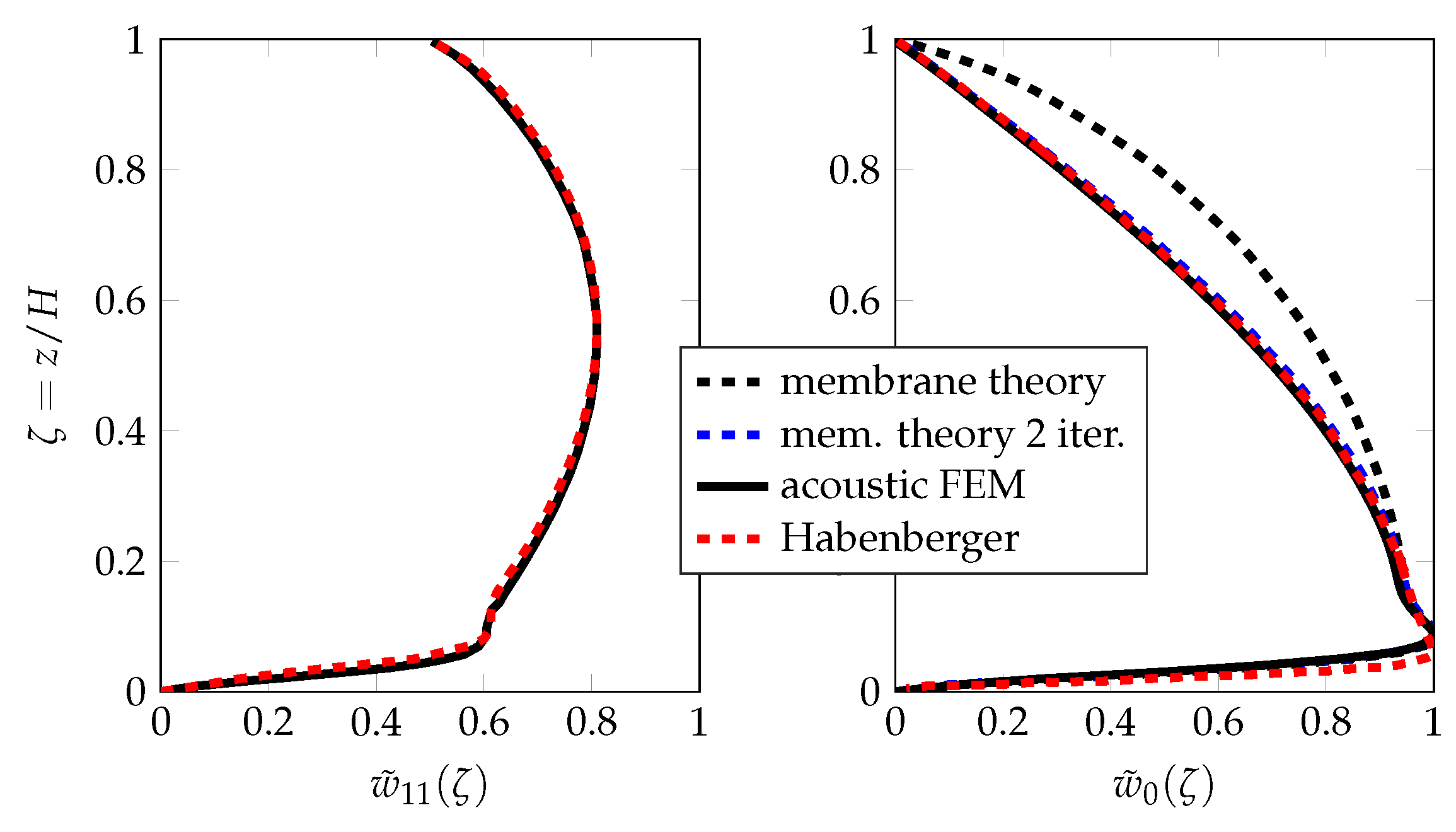
3.3. Comparative Verification

In order to evaluate the suitability of the method, an ideal tank of a constant thickness, with a perfectly cylindrical geometry and with the following characteristics, was taken as a reference:

• Radius $R=20$ m;
• Wetted height $H=20$ m coincident with the height of the freeboard;
• Liquid content: water $\rho =995$ kg/m³, $K_f=2.1$ GPa;
• Steel shell, $E=210$ GPa, $\nu =0.33$, $\rho =7800$ kg/m³;
• Constant thickness, $s=0.025$ m.

We have to define the material properties for the realized geometries, and the fluid will be provided with acoustic properties. In this case, we choose to model the compressibility by defining only the modulus $K_f$; the fluid will therefore be inviscid and without volumetric resistance.

Next, the thickness of the elements of the cylindrical shell must be defined; for the liquid, a solid section is defined by associating it with the liquid material.

Having defined the model by adding the interactions and boundary conditions, it only remains to generate the mesh and assign the element type. The finished model complete with the mesh is shown in Figure 9.

It is possible to observe that the mode with the highest participation factor and participant mass along the x-direction is mode 7, corresponding to a frequency of 3.94 Hz, and it can be seen from the deformations in Figure 10 (red shows the areas of maximum deformation), that this is the first anti-symmetrical mode.

As shown in Figure 11, the modal deformations obtained from the acoustic modal analysis coincide with those obtained through semi-analytical methods in the simplified case of a perfectly cylindrical geometry and constant thickness.

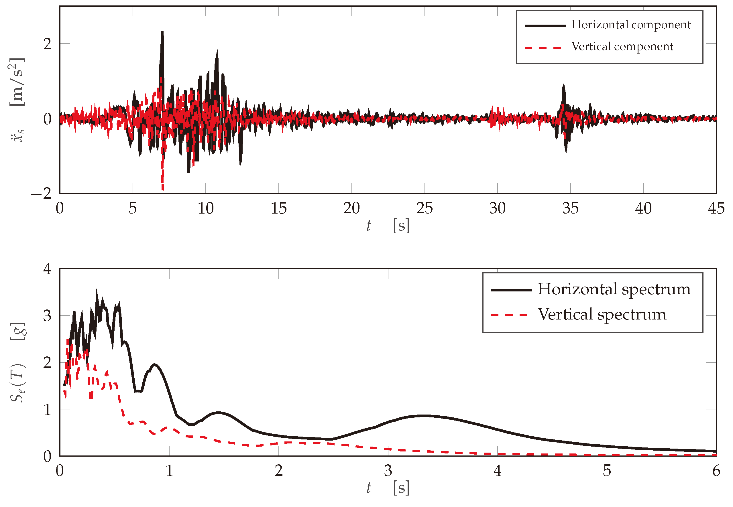
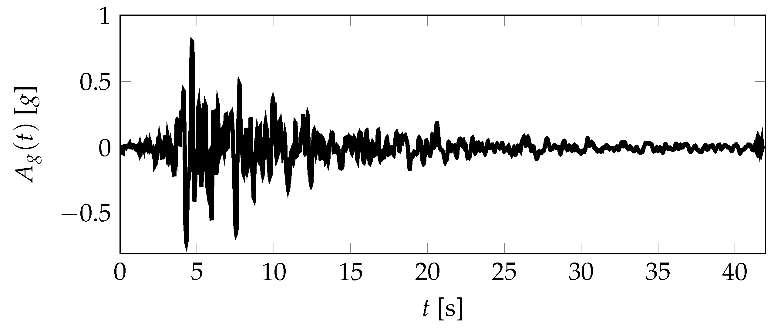
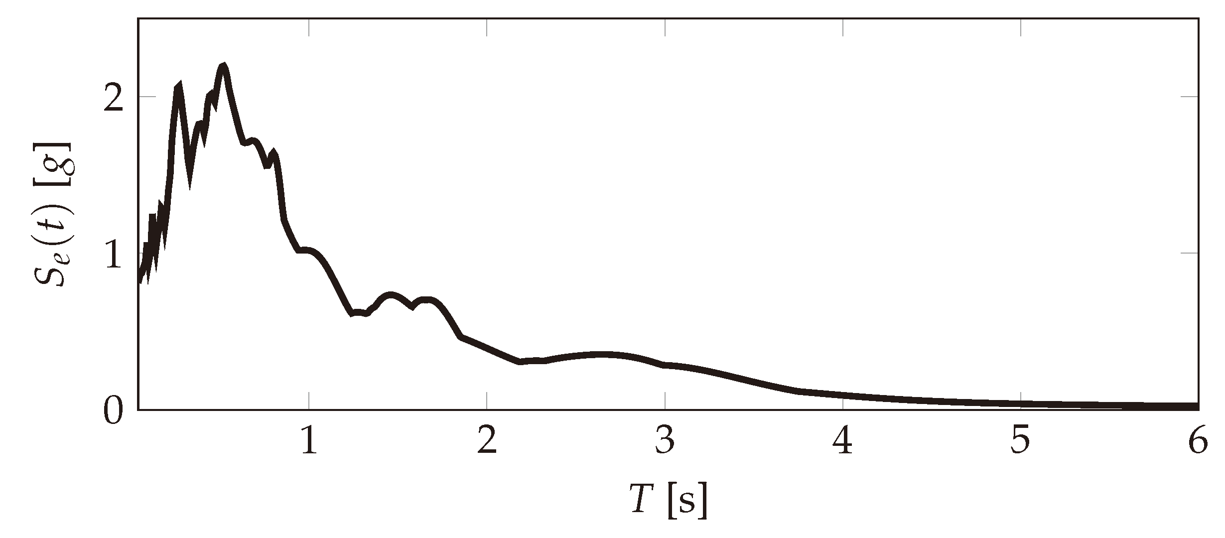
4. Case Study

In order to consider an application case, the fixed conical roof tank of a medium-sized tank from a petroleum refinery plant in the Turkish province of Kocaeli was analyzed. The following two levels of seismic ground motion are defined in the Turkish norm [1] for ultimate limit states.

• Earthquake Ground Motion Level 1 (DD-1): characterizes a very rare seismic event where the corresponding return period is 2475 years.
• Earthquake Ground Motion Level 2 (DD-2): characterizes a rare seismic event where the corresponding return period is 475 years.

The analysis was also carried out on another accelerogram, adapted to the DD-2 level, for the 1981 Alkion earthquake in Greece. The adapted accelerogram and elastic response spectrum are shown in Figure 12 and Figure 13.

The tank under analysis is used for the storage of light distillation naphtha and is equipped with a fixed conical roof and a single-layer internal floating roof with honeycomb panels. The analysis of the floating roof can be carried out by means of analytical and numerical approaches, based on potential flow theory and found in the literature [23,24]. The characteristics and main design parameters of the tank are summarized in

Table 1. Summary table of tank design parameters.

Tank Design Data
Tank diameter [m]	27.50
Tank height (filling) [m]	13.50
Tank height (geometric) [m]	15.00
Design density of content [kg/m3]	750.00

.

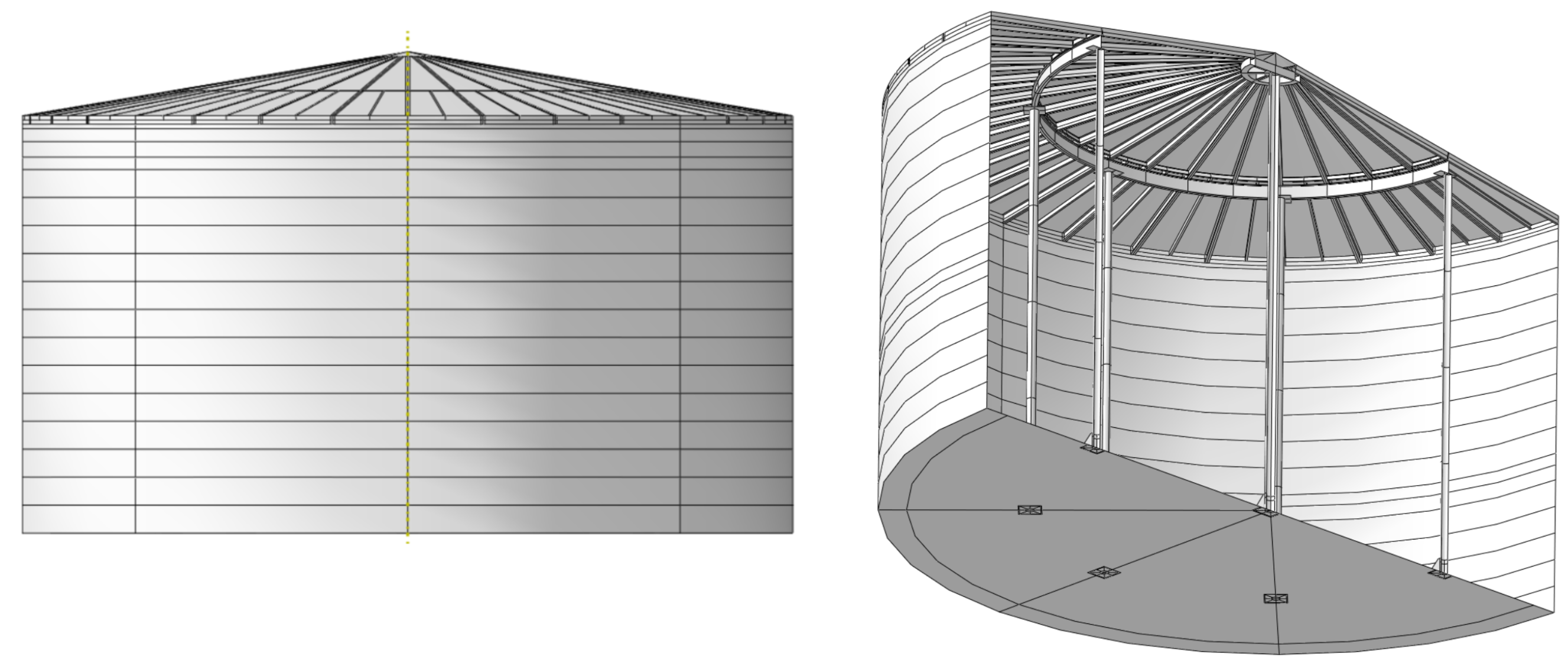
4.1. Ideal Model

In order to simplify the modeling of the assembly and to allow for greater regularity of the mesh, the beams running in a circular direction were modeled as a single curvilinear beam. The radial beams, on the other hand, were modeled by trying to respect the actual dimensions as much as possible.

The shell was realized as a surface of revolution and appropriately partitioned into sixteen rings in order to be able to assign the sections with their relative thicknesses. Figure 14 shows the ideal partitioned model and some details of the roof, shown in a cross-section and isometric view.

All calculated loads were applied in the same non-linear load step after an elastic–linear step in which only the hydrostatic component and the gravitational load were applied.

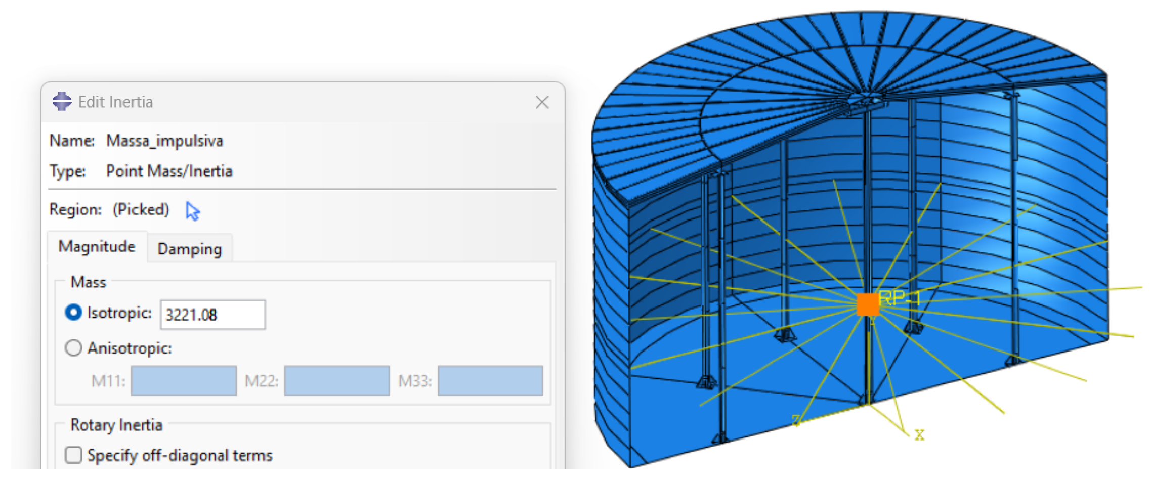
4.2. Impulsive Rigid Contribution

For the calculation of the frequencies required for the integration of the SDOF relating to the impulsive rigid contribution, a subsection was created on the mantle at a height

$$h_i=5569.17\mathrm{mm}$$

(17)

calculated by relation (9), in order to perform a modal analysis by coupling a concentrated mass to the shell (the model developed is shown in Figure 15),

$$m_i=3221.08\mathrm{tonn}$$

(18)

calculated according to relation (7).

The modal analysis returns a frequency for the first rigid impulsive mode equal to $f_i=8.18\mathrm{Hz}$ (Figure 16).

Using this frequency to integrate the one-degree-of-freedom oscillator yields a corresponding spectral response of $S_a\left(T_i\right)=2.5967g$. The corresponding pressure distribution is obtained from (5) using the value of the spectral response instead of the acceleration value $A_g\left(t\right)$; the pressure curve calculated at the outer radius ($r=R$) and at the base ($z=0$), along the seismic direction of action ($\theta =0$), is shown in Figure 17.

4.3. Convective Contribution

The contribution from the free-surface oscillation is calculated with the relations seen above, considering only the first anti-symmetric mode. The convective acceleration obtained by integrating the oscillator at one degree of freedom is $A_{c1,\max }\simeq 1.34$ m/s², to which corresponds a pressure distribution that can be calculated using (11) and is shown in Figure 18 for $\theta =0$ along the walls and along the base.

4.4. Deformability Contribution

In order to perform the acoustic modal analysis, the only change to be made to the model is the addition of the internal liquid domain, which must be partitioned like the mantle to allow the superposition of the external nodes when generating the mesh.

The acoustic modal analysis returns an anti-symmetric first mode frequency of $f_{f1}\simeq 5.77$ Hz.

The deformation values, shown with a color map in Figure 19, can be extracted using Abaqus/CAE 2022.

By normalizing the extracted values to the maximum displacement, the axial deformation $f\left(\zeta \right)$ necessary for the calculation of the impulsive–flexible pressure distribution is finally obtained by using (16), as shown in Figure 20.

4.5. Deformed Model

Having obtained the scanned surface, it was possible to import it as a set of points into Abaqus/CAE 2022, Figure 21.

The imported surface replaces the cylindrical shell with the ideal geometry Figure 22.

4.6. Setting Up Analyses

The material properties are summarized in

Table 2. Table of tank materials.

Assigned Materials
Material	${\mathit{\sigma }}_{\mathit{y}}$ [MPa]	${\mathit{\epsilon }}_{\mathit{u}}$	${\mathit{\sigma }}_{\mathit{u}}$ [MPa]	$\mathit{E}$ [GPa]	${\mathit{\rho }}_{\mathit{m}}$ [kg/m3]	$\mathit{\nu }$
A283-gr. C	235	0.11	236	210	8000	0.3
R-ST-37-2	235	0.11	236	210	8000	0.3
SA106-gr. B	241	0.11	242	210	8000	0.3

.

Two load steps are defined in addition to the initial step.

• Generic static step: in this step, the hydrostatic load and the force of gravity are applied with linear progression; in this step, it is required to update the stiffness matrix by including the geometric non-linearities, a calculation necessary in the regime of large displacements.
• Incremental non-linear static step: in this step, the hydrodynamic loads are applied and the analysis is carried out using the modified Riks method.

The model (Figure 23) mesh contains 198,127 nodes from 199,474 quadrangular (S4R) and a small number of triangular (S3) shell elements with a linear formulation.

5. Results

The non-linear analyses in both cases were progressed to a maximum number of 100 increments; the output variables collected were as follows:

• Load proportionality factor $\lambda$;
• Constraining reaction $R{F}_x$ of the central node of the base along the direction of the load;
• Moment modulus $RM$ reaction of the central node of the base;
• Displacement $U_{\mathrm{el}}$ of the node that exhibits the greatest displacement at the beginning of the non-linear step;
• Displacement $U_{\mathrm{pl}}$ of the node that exhibits the greatest displacement in the non-linear step.

5.1. Static Step

In the first step, only the hydrostatic load and the acceleration of gravity are applied, which gives the weight of the structural components. The maximum initial displacement of the non-linear analysis at the end of the static step is 45.91 mm.

The stresses will start from values of around 100 MPa at base, with several zones of intensification due to the imperfections of the deformed shell but no zones of plasticity as shown in Figure 24.

It can be verified with the approaches of the norm that elastic buckling does not occur under such conditions and therefore the tank is verified for stationary conditions.

In particular, using the approach described in EC8 in paragraph A.10.2, it is necessary to verify that, for the region in which both the minimum pressure and minimum thickness are located, the axial tension ${\sigma }_z$ does not exceed a certain limit value, calculated by means of a semi-analytical formula (Rotter’s formula [25]). In particular, we have

$${\sigma }_{\lim }=0.19·{\sigma }_{\mathrm{cl}}+0.81{\sigma }_p$$

(19)

5.2. Non-Linear Step, Seismic Case DD1

At the end of the non-linear step, elastic buckling is observed on the depression side, below the free surface (Figure 25).

This type of damage (red zone) is observed in tanks subjected to seismic stress, such as the one shown in Figure 26 for a qualitative comparison of the analysis results.

The deformed configuration of Figure 25 is the one that is obtained at the end of the analysis; however, buckling already occurs at the eighth increment, as shown in Figure 27.

The buckling occurs at a height of about 12 m with axial tension around 54 MPa; in fact, evaluating (19) for the corresponding thickness (7 mm) and the minimum possible internal pressure from the seismic component, we obtain

$$p_{\min }=p_{\mathrm{tot}}(\zeta =12/H,\theta =\pi )\simeq -135,760\mathrm{Pa}\Rightarrow {\sigma }_{\lim }\simeq 53.6\mathrm{MPa}$$

On the pressure side, it can be seen in Figure 28 that yield zones already occur at the fifth increment.

By evaluating the plastic deformation at the last increment, it can be observed in Figure 29 that the plasticized zones are very localized and of low magnitude and extension.

Therefore, in this case, it can be assumed that the collapse of the structure under the seismic conditions related to the seismic event DD1 is mainly dependent on elastic buckling caused by load asymmetry.

It is also interesting to evaluate the behavior of the structure after buckling, which can be obtained from the value of the base shear. In Figure 30, the curve $R{F}_x-U_{\max }$ shows the value of the constraint reaction $R{F}_x$ in the direction of application of the seismic load; $U_{\max }$ is the maximum displacement between $U_{\mathrm{el}}$ and $U_{\mathrm{pl}}$.

It can be observed that, after the occurrence of buckling, the structure shows a resistance capacity up to a maximum point beyond which there is a decrease in load. As the analysis progresses, a snap-back phenomenon is also observed, which can be verified to be localized in the buckling trigger zone.

5.3. Non-Linear Step, Seismic Case DD2

In the second seismic case for the damage limit state, the structure exhibits extensive plastic deformation on the pressure side (Figure 31), with the formation of a circumferential protrusion at a medium to low height; this damage mode has also been observed under real conditions Figure 32.

From the force–displacement curve Figure 33, constructed similarly to the previous case, the structure shows residual capacity, but the shear value tends to stabilize towards a value of approximately 3.6 × 10⁷ N.

6. Conclusions

The approach proposed in this work is based on coupled acoustic modal analysis [17,18], which allows the fundamental seismic stress mode of the fluid–structural system to be obtained. This introduces the possibility of starting from a model that already takes into account the variability in thickness, the presence of roof structures, and other geometric complexities in the calculation of coupled modes.

Once the load distribution to be applied is resolved, the same model can be used in non-linear analysis, with the possibility of including the geometric imperfections of the actual shell surface, obtained from three-dimensional scans or other measurements performed in the field.

It should be noted, however, that in order to comprehensively understand the seismic response of the structure, the most complete approach would involve performing non-linear dynamic analyses in a significant number of load cases and conditions. However, this type of analysis is complex and difficult to implement in practice, mainly due to the complexity of the parameters influencing the results and the large number of runs needed.

In this regard, the use of non-linear static analyses is seen, even in the most recent technical standards, as an attractive approach in terms of the calculation time and interpretation, because it enables the modeling of the structural response through the extrapolation of a force–displacement link, i.e., a representative capacity curve (also called a pushover curve) [26,27].

In this way, the response of the structure can be related to a simpler system with a few degrees of freedom (or a joystick model), providing an evaluation of the stiffness that characterizes it (in terms of load–displacement ratios) and taking into account the non-linear behavior that occurs after the collapse modes that are typical of the structure. Consequently, a more accurate predictive estimate of the seismic response is possible in comparison to the simplified, purely theoretical models [28,29].

These reduced models, which are, in any case, more easily produced and analyzed than full-order models, can subsequently be used to generate a much larger number of performance statistical points, which may be necessary for the processing and reliable evaluation of the seismic risks of tanks.

References

- Turkish Ministry of Construction and Settlement. Design Code for Buildings in Seismic Regions; Turkish Ministry of Construction and Settlement: Ankara, Türkiye, 2018. [Google Scholar]
- Jacobsen, L.S. Impulsive hydrodynamics of fluid inside a cylindrical tank and of fluid surrounding a cylindrical pier. Bull. Seismol. Soc. Am. 1949, 39, 189–204. [Google Scholar] [CrossRef]
- Housner, G.W. Dynamic pressures on accelerated fluid containers. Bull. Seismol. Soc. Am. 1957, 47, 15–35. [Google Scholar] [CrossRef]
- Housner, G.W. The dynamic behavior of water tanks. Bull. Seismol. Soc. Am. 1963, 53, 381–387. [Google Scholar] [CrossRef]
- Fischer, F.D.; Rammerstorferf, F.G.; Scharf, K. Earthquake Resistant Design of Anchored and Unanchored Liquid Storage Tanks Under Three-Dimensional Earthquake Excitation; Springer: Berlin/Heidelberg, Germany, 1991; pp. 317–371. [Google Scholar]
- Fischer, F.D.; Rammerstorfer, F.G. A refined analysis of sloshing effects in seismically excited tanks. Int. J. Press. Vessel. Pip. 1999, 76, 693–709. [Google Scholar] [CrossRef]
- Cai, Z.; Topa, A.; Djukic, L.P.; Herath, M.T.; Pearce, G.M. Evaluation of rigid body force in liquid sloshing problems of a partially filled tank: Traditional CFD/SPH/ALE comparative study. Ocean. Eng. 2021, 236, 109556. [Google Scholar] [CrossRef]
- Caprinozzi, S.; Paolacci, F.; Dolšek, M. Seismic risk assessment of liquid overtopping in a steel storage tank equipped with a single deck floating roof. J. Loss Prev. Process Ind. 2020, 67, 104269. [Google Scholar] [CrossRef]
- Souli, M.; Kultsep, A.V.; Al-Bahkali, E.; Pain, C.C.; Moatamedi, M. Arbitrary Lagrangian Eulerian formulation for sloshing tank analysis in nuclear engineering. Nucl. Sci. Eng. 2016, 183, 126–134. [Google Scholar] [CrossRef]
- Ozdemir, Z.; Souli, M.; Fahjan, Y.M. FSI methods for seismic analysis of sloshing tank problems. Mech. Ind. 2010, 11, 133–147. [Google Scholar] [CrossRef]
- Kang, T.W.; Yang, H.I.; Jeon, J.S. Earthquake-induced sloshing effects on the hydrodynamic pressure response of rigid cylindrical liquid storage tanks using CFD simulation. Eng. Struct. 2019, 197, 109376. [Google Scholar] [CrossRef]
- Caron, P.; Cruchaga, M.; Larreteguy, A. Study of 3D sloshing in a vertical cylindrical tank. Phys. Fluids 2018, 30, 082112. [Google Scholar] [CrossRef]
- Cao, X.; Ming, F.; Zhang, A. Sloshing in a rectangular tank based on SPH simulation. Appl. Ocean. Res. 2014, 47, 241–254. [Google Scholar] [CrossRef]
- Rafiee, A.; Pistani, F.; Thiagarajan, K. Study of liquid sloshing: Numerical and experimental approach. Comput. Mech. 2011, 47, 65–75. [Google Scholar] [CrossRef]
- Wiśniewski, A.; Kucharski, R. Eigencharacteristics of fluid filled tanks: An extended symmetrical coupled approach. TASK Q. 2006, 10, 455–468. [Google Scholar]
- Phan, H.N.; Paolacci, F. Fluid-structure interaction problems: An application to anchored and unanchored steel storage tanks subjected to seismic loadings. arXiv 2018, arXiv:1805.00679. [Google Scholar]
- Rawat, A.; Matsagar, V.; Nagpal, A.K. Seismic Analysis of Steel Cylindrical Liquid Storage Tank Using Coupled Acoustic-Structural Finite Element Method For Fluid-Structure Interaction. Int. J. Acoust. Vib. 2020, 25, 27–40. [Google Scholar] [CrossRef]
- Dhulipala, S.L.N.; Bolisetti, C.; Munday, L.B.; Hoffman, W.M.; Yu, C.C.; Mir, F.U.H.; Kong, F.; Lindsay, A.D.; Whittaker, A.S. Development, verification, and validation of comprehensive acoustic fluid-structure interaction capabilities in an open-source computational platform. Earthq. Eng. Struct. Dyn. 2022, 51, 2188–2219. [Google Scholar] [CrossRef]
- Veletsos, A.S. Seismic effects in flexible liquid storage tanks. In Proceedings of the 5th World Conference on Earthquake Engineering, Rome, Italy, 25–29 June 1973; Bulletin of the Seismological Society of America: McLean, VA, USA, 1974; Volume 1, pp. 630–639. [Google Scholar]
- Balendra, T.; Ang, K.K.; Paramasivam, P.; Lee, S.L. Free vibration analysis of cylindrical liquid storage tanks. Int. J. Mech. Sci. 1982, 24, 47–59. [Google Scholar] [CrossRef]
- Flügge, W. Stresses in Shells; Springer Science & Business Media: Berlin/Heidelberg, Germany, 1973. [Google Scholar]
- Habenberger, J. Beitrag zur Berechnung von nachgiebig gelagerten Behältertragwerken unter seismischen Einwirkungen. Ph.D. Thesis, Bauhaus-Universität Weimar, Weimar, Germany, 2001. [Google Scholar]
- Chiappelloni, L.; Belardi, V.; Serraino, F.; Trupiano, S.; Gaetani, L.; Vivio, F. Structural behaviour of single-deck floating roof tanks subject to seismic loading. IOP Conf. Ser. Mater. Sci. Eng. 2024, 1306, 012002. [Google Scholar] [CrossRef]
- Goudarzi, M.A. Seismic behavior of a single deck floating roof due to second sloshing mode. J. Press. Vessel. Technol. 2013, 135, 011801. [Google Scholar] [CrossRef]
- Rotter, J. Buckling of ground-supported cylindrical steel bins under vertical compressive wall loads. In Proceedings of the Metal Structures Conference, Melbourne, Australia, 23–24 May 1985; p. 16. [Google Scholar]
- Causevic, M.; Mitrovic, S. Comparison between non-linear dynamic and static seismic analysis of structures according to European and US provisions. Bull. Earthq. Eng. 2011, 9, 467–489. [Google Scholar] [CrossRef]
- Bosco, M.; Ghersi, A.; Marino, E.M. On the evaluation of seismic response of structures by nonlinear static methods. Earthq. Eng. Struct. Dyn. 2009, 38, 1465–1482. [Google Scholar] [CrossRef]
- Bakalis, K.; Kazantzi, A.K.; Vamvatsikos, D.; Fragiadakis, M. Seismic performance evaluation of liquid storage tanks using nonlinear static procedures. J. Press. Vessel. Technol. 2019, 141, 010902. [Google Scholar] [CrossRef]
- Bal, I.E.; Smyrou, E. Implementation of Emerging Technologies in Seismic Risk Estimation. In Proceedings of the European Conference on Earthquake Engineering and Seismology, Bucharest, Romania, 4–9 September 2022; Springer: Berlin/Heidelberg, Germany, 2022; pp. 279–294. [Google Scholar]